
Abstract
This article presents a probabilistic structural identification of the Tamar bridge using a detailed finite element model. Parameters of the bridge cables initial strain and bearings friction were identified. Effects of temperature and traffic were jointly considered as a driving excitation of the bridge’s displacement and natural frequency response. Structural identification is performed with a modular Bayesian framework, which uses multiple response Gaussian processes to emulate the model response surface and its inadequacy, that is, model discrepancy. In addition, the Metropolis–Hastings algorithm was used as an expansion for multiple parameter identification. The novelty of the approach stems from its ability to obtain unbiased parameter identifications and model discrepancy trends and correlations. Results demonstrate the applicability of the proposed method for complex civil infrastructure. A close agreement between identified parameters and test data was observed. Estimated discrepancy functions indicate that the model predicted the bridge mid-span displacements more accurately than its natural frequencies and that the adopted traffic model was less able to simulate the bridge behaviour during traffic congestion periods.
Keywords
Introduction
Critical civil infrastructure, such as long suspension bridges, represents a capital investment from communities and local governments. Therefore, its serviceability fully justifies dedicated long-term monitoring systems. structural health monitoring (SHM) 1 concerns the design, deployment, maintenance of structural monitoring systems and subsequent data interpretation.
Relative to data interpretation, the actual structural behaviour is often grossly misinterpreted when compared against the input–output relation of a physics-based computer model. 2 In other words, structural identification (st-id) is very susceptible to uncertainties. These uncertainties stem from experimental and conceptual factors, such as the high heterogeneity of monitored data or model discrepancy, that is, modelling assumptions and simplifications.
Several probabilistic st-id methodologies,3,4 such as Kalman filters 5 or fuzzy logic, 6 have been used to address these uncertainties. Another example is Bayesian methods, which have been introduced to the SHM community by Sohn and Law, 7 Beck and Katafygiotis, 8 and Beck and Au. 9 Unfortunately, the frameworks proposed by these authors are not well suited to address the confounding influences due to environmental (temperature, wind) and operational (traffic, pedestrians) actions.10–13 Recently, Behmanesh et al. presented a hierarchical Bayesian framework,14,15 which, in the absence of noise or model discrepancy, accurately identifies parameters subjected to external actions. 16
Thus, in addition to environmental/operational effects, model discrepancy is the main challenge hindering these methodologies. According to the principle of maximum entropy, 17 this source of uncertainty has recurrently been assumed as a zero-mean uncorrelated Gaussian.18–22 Such assumption is reasonable as a conservative upper limit, but it brings considerable shortcomings. Namely, it introduces parameter inference bias and negates the possibility of finding patterns and correlations, which are vital for model updating and performance assessment. Authors, such as Goulet and Smith 3 or Papadimitriou and Lombaert, 23 have highlighted the benefits of weakening such assumptions for st-id and measurement system design, respectively.
The main alternative to physics-based models is an interpretation with data-based models,24,25 which is not bound by physical laws and thus can approximate data patterns more efficiently without model discrepancy. Examples include clustering 26 or Gaussian mixture 27 models, which are used for damage identification using Bayesian inference. However, data-based models have a limited ability for extrapolation and thorough explanation of data trends. Finally, hybrid models gather both, a descriptive coherency of a structural system, and adaptability for identification of unusual data patterns.
Consequently, the current contribution applies a different approach to the problem of st-id. The framework under focus is a hybrid modular Bayesian approach (MBA) developed based on the method proposed by Kennedy and O’Hagan. 28 Previous work by Jesus et al. 29 highlighted an application of the MBA to a reduced-scale aluminium bridge (under temperature variation only). The work however was restricted to the identification of a single parameter. If model discrepancy is approximated with a multiple response Gaussian process (mrGp), then probabilistic st-id in SHM is expected to improve. Therefore in this article, encouraged by the previous work, an expansion of the MBA using the Metropolis-Hasting algorithm for multiple parameters identification is presented. This article also details the first application of the method to a full-scale structure, the Tamar long suspension bridge, under temperature and traffic loading.
Enhanced MBA
In this section, a short summary of the MBA and relevant details of its enhancement for multi-parameter identification are presented. For the remainder of this work Table 1 is to be used as a nomenclature table.
Table of notation.
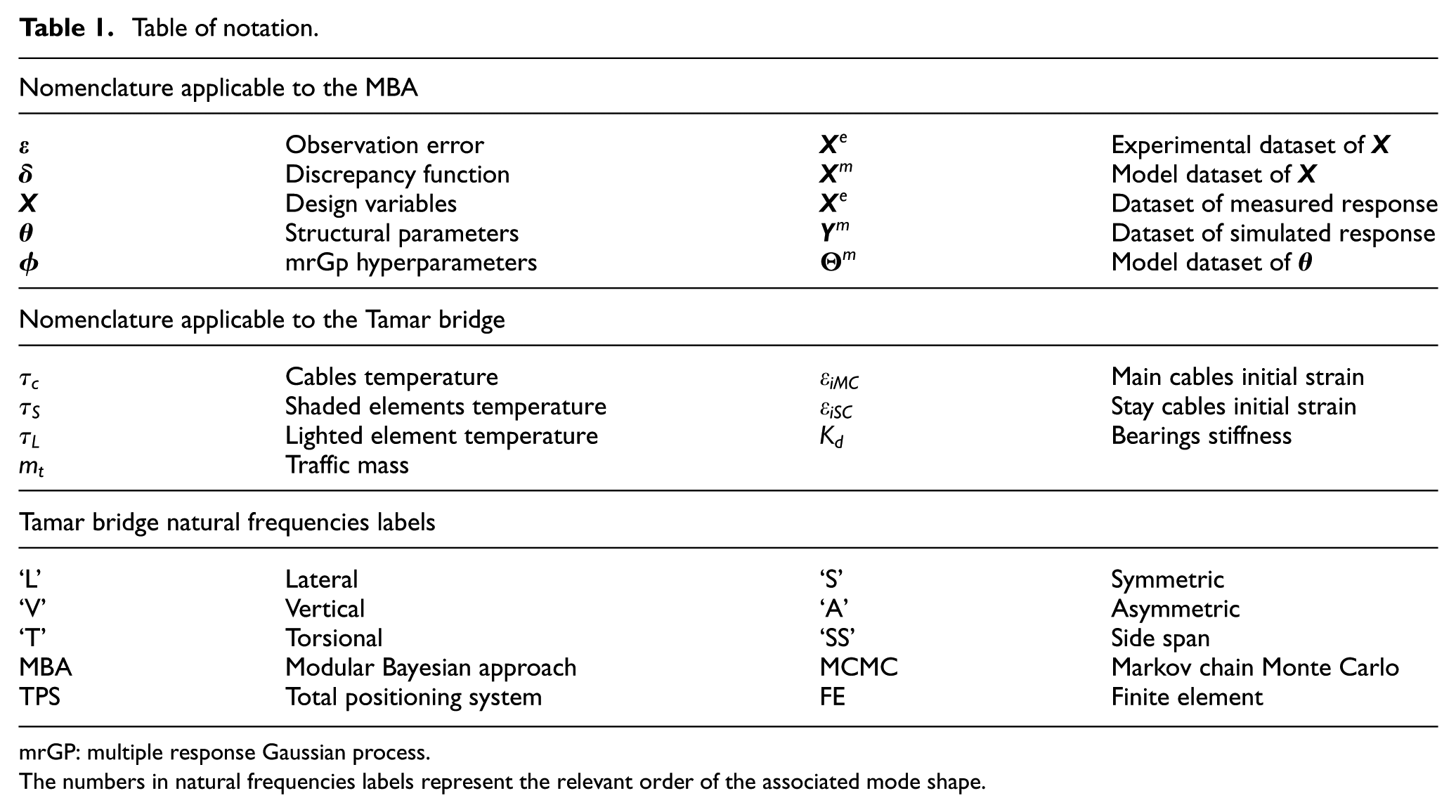
mrGP: multiple response Gaussian process.
The numbers in natural frequencies labels represent the relevant order of the associated mode shape.
The original MBA formulation was developed for a single response case,28,30 that is, only considering predictions of one model output function. Arendt et al. 31 proved that, unless under some specific conditions, the single response case fails to identify the true structural parameters. Instead, a multiple response formulation which allows for a more informative data model has been proposed. 32
General workflow of the MBA
The MBA aims to solve an equation of model calibration, which can be written as follows

where
There are an infinite number of solutions of equation (1). For different values of the parameters
Finally, Bayes’ theorem can be used to update the belief on the structural parameters as follows
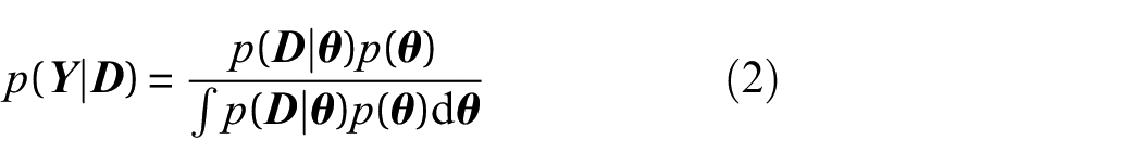
where
The MBA breaks the complete process described above into four modules, hence the name MBA. For a flowchart of the algorithm, see Figure 1. In modules 1 and 2, the model response surface and the discrepancy function are fitted by statistical models, known as mrGp, whose parameters (hyperparameters
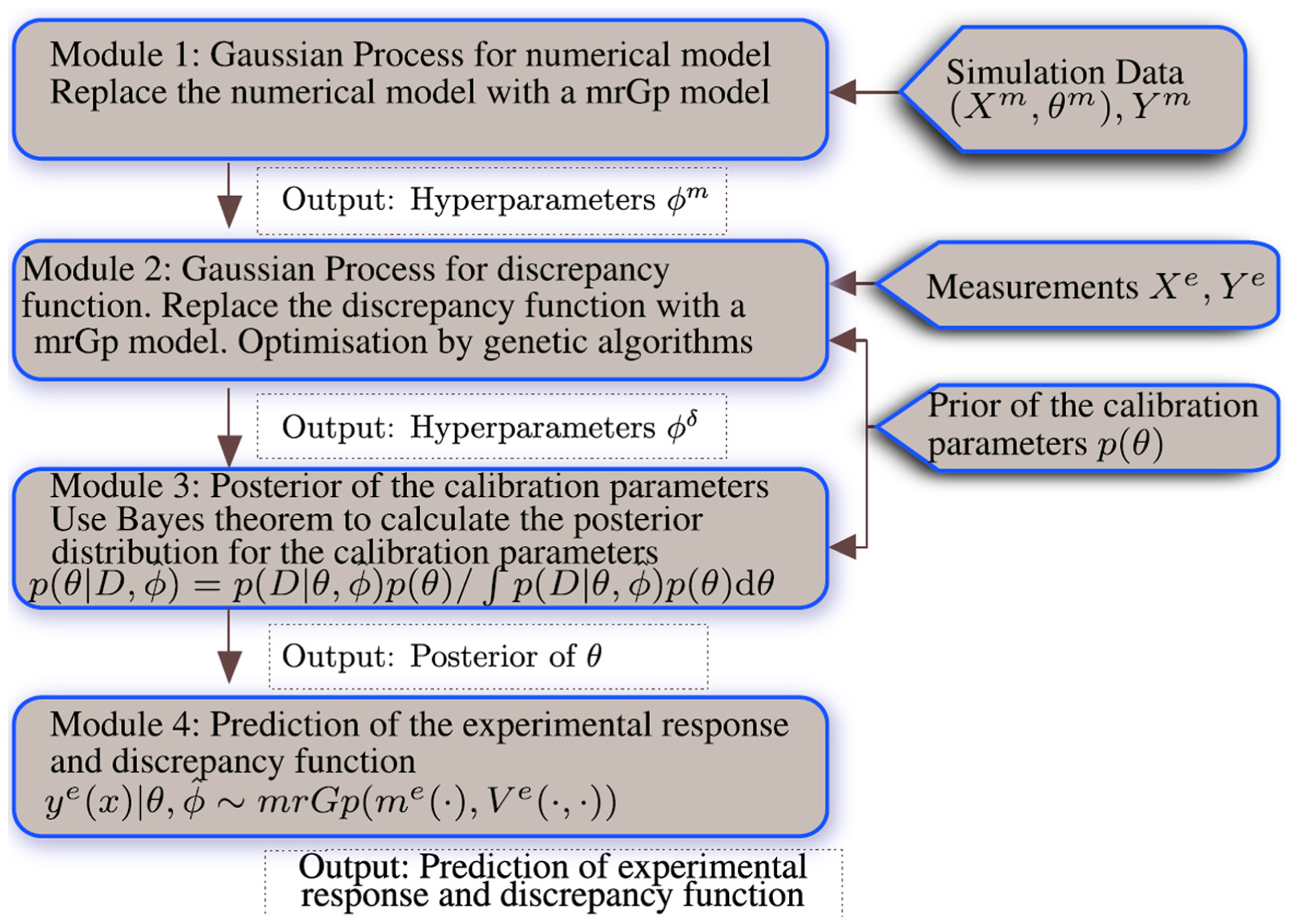
Flowchart of the modular Bayesian algorithm.
In module 3, the estimated hyperparameters of the mrGps become fixed and are used to set up a global data model, the likelihood function, that explains both simulations and observations for a set of given structural parameters
Note that such a modular separation will greatly reduce the computational effort required to solve equation (1), comparatively to other Bayesian frameworks. It implies that the uncertainty effects are not considered fully. As a drawback, identification of true parameters is more challenging. However and as established by Arendt et al., considering multiple responses considerably improves the identifiability of the MBA.
The next section presents an enhancement over the above described formulation.
Markov chain Monte Carlo sampling of posterior distribution
Previous implementations of the MBA are limited to identification of a single structural parameter. This section discusses a Markov chain Monte Carlo (MCMC) routine which allows to identify multiple parameters with the MBA. The Gauss–Legendre has been used for the single-parameter case, whereas our implementation includes a routine based on the Metropolis–Hastings (MH) algorithm.33,34 MCMC methods are commonly used to address multi-dimensional integrals which occur in fields such as Bayesian inference. 9
Since the likelihood of the MBA is multivariate normal and analytically untractable, numerical methods are required to perform its integration. The MH algorithm is known to converge to a target distribution for an increasing number of samples. Specifically, the target distribution has been assumed as symmetric and sampled with a 3000 burn-in period for a total of 100,000 samples. A standard multivariate normal distribution
Although it is acknowledged that the MH algorithm has its limitations, and an alternative such as the adaptive Metropolis algorithm would be more suitable, 35 the aim is to showcase the potential of the MBA to identify multiple parameters and motivate further developments. In the following sections, its performance shall be illustrated with an application to the Tamar long suspension bridge.
Tamar bridge experimental and simulated dataset
This section presents the Tamar bridge’s SHM system, the monitored data under consideration and the finite element (FE) model developed to study its behaviour.
Tamar bridge is a 335-m-long suspension bridge, built in 1959 and reconstructed between 1999 and 2001, where a larger side deck and stay cables have been added, see Figure 2 for a reference. Two long-term monitoring systems have been installed and several localised expeditions have been carried out through time for reliability assessment.
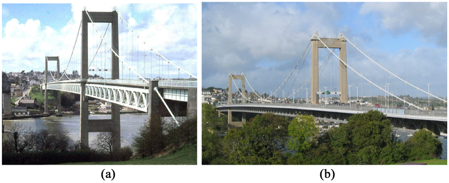
Tamar suspension bridge (a) before (1978) 36 and (b) after (2018) its reconstruction in the late 1990s. Note the larger deck and stay cables added in 2001.
In addition, an FE model was developed by Westgate 37 to study environmental and operational effects on its structural performance. It is worth mentioning the following excerpt ‘In fact, Tamar Bridge has so far presented a challenging case study for model calibration, lending support to the view that no single model provides a perfect representation of a structure when matched to provided experimental data’. 38
On the basis of the present methodology and data/model, three key properties relevant for stake holders will be estimated. One is the friction in the thermal expansion bearings of Saltash tower, which can lead to deck cracks and further structural anomalies. The remaining two properties are the initial strain in the main and stay cables of the bridge. The initial strain is defined as the strain relative to when the bridge cables have been installed initially, that is, containing all the load-history that the cables have supported since installation. Its increase could indicate internal damage, such as broken wires, corrosion, cracks and wear.
Monitored data and post-processing
It is important to establish which design variables are relevant to study Tamar bridge’s dynamic behaviour. A study from Cross et al. 39 indicates that traffic, temperature and wind have the most influence on Tamar bridge natural frequencies, by decreasing order of relevance. However, this study will be limited to the effects of traffic and temperature.
In the absence of the above information, a normal procedure would include the following:
Monitor the structural behaviour for a certain period of time, preferably at least for a year period;
Analyse existent correlations between environmental/operational effects and the structural output, displacements, vibration data, and so on;
Select the effects which have the highest influence on the structural output and consider them during the modelling process.
Several sensors have been installed through time on Tamar bridge, but for the purpose of this study, we considered data which were monitored from a set of accelerometers, a total positioning system (TPS) reflector and thermocouples, which are shown in Figure 3. The available data also include vehicle counts from toll gates of the Plymouth side.
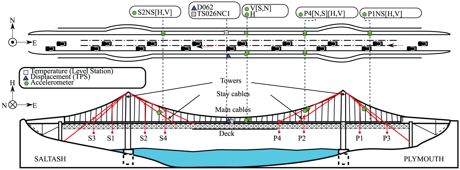
Diagram of Tamar bridge SHM system – cable temperature sensor, displacement reflector and accelerometers from whose natural frequencies/mode shapes are estimated. There are 16 stay cables on North/South and Saltash/Plymouth sides.
The monitoring period ranged from May 2009 to March 2010, where synchronised temperature, traffic and modal data were found to be richer. Furthermore, a year time-frame was assumed as a good reference for calibration/validation of the FE model, since it covers seasonal variations. Relevant post-processing operations will now be detailed.
First, the natural frequencies of the structure were determined with a stochastic subspace identification (SSI) technique, 40 based on available acceleration data. Specifically, at each half-hour, 10-min acceleration recordings were post-processed to determine the natural frequencies and mode shapes of the infrastructure. Second, displacements at the middle span of the bridge in three directions, vertical, East and North, were obtained from the TPS.
After the above-mentioned operations, a 2419 points dataset was obtained, which is visualised in Figure 4. Visible trends indicate linear correlations, except for the traffic/displacement relation in Figure 4(d). Therefore, a linear correlation function (or kernel) was assumed for the mrGps that fit the discrepancy function and the FE model. 41 Furthermore, the zero displacements at highest temperatures in Figure 4(c) and (d) occur because the data have been offset relative to the highest peak of temperature × traffic load. Frequency labels follow the convention: ‘L’ is a lateral mode shape, ‘V’ is vertical mode shape, ‘T’ is a torsional mode shape, ‘TRANS’ is a longitudinal translation mode, ‘S’ is symmetric, ‘A’ is asymmetric, ‘SS’ is side span and the numbers are their relevant order.
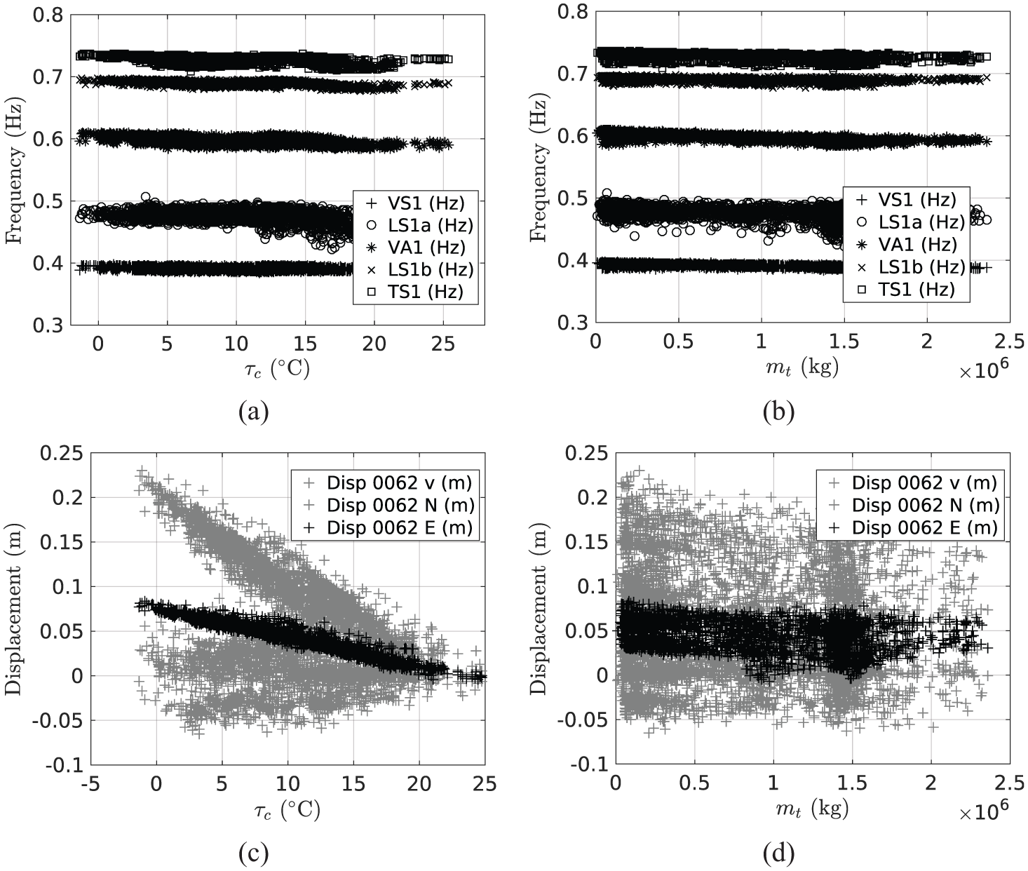
Post-processed data – May of 2009 to March of 2010 time period: (a, b) natural frequencies and (c, d) mid-span relative displacements.
For future reference, it is worth mentioning some relevant information related to the bridge main and stay cables. Namely, the main suspension cables are made from 31 locked coil wire ropes, each 60 mm in diameter, and the overall diameter of the main cable is 380 mm, resulting in a cable cross-sectional area of 882.36 cm2. The stay cables indicated in Fig. 3 have areas of 87.01 cm2 for S2 and P2 (110 mm diameter strands) and 70.74 cm2 for the remaning cables (102 mm diameter strands).
Modelling of thermal and traffic effects
In this section, Tamar bridge FE model will be briefly described, along with to-be-identified structural parameters, and modelling aspects of its dynamic behaviour in the presence of traffic and thermal variations.
The FE bridge model has been developed using ANSYS Parametric Design Language (APDL) source code 42 and consists of approximately 45,000 elements, from which expansion joints have been modelled with linear spring elements, truss members with fixed-rotation beams, deck/towers with shells and the cables and hangers with uniaxial tension only beam elements.
First, it is important to discriminate the three parameters which will be identified. One is the stiffness of linear springs
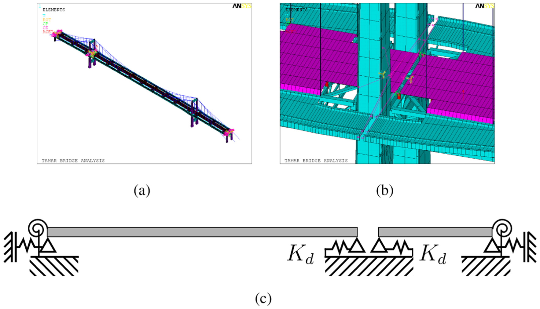
Tamar bridge FE model and detail of imposed constraints simulated as linear spring elements. (a) Perspective view, (b) expansion gap at Saltash tower and (c) bridge boundary conditions diagram.
For each cable type (main or stay), the initial strain is assumed constant along the cable length and across all cables. The Young’s modulus of the cables was assumed as 155 GPa, and the initial strain
Second, after having detailed the model parameters, it is now necessary to highlight how temperature effects have been considered. For the present work, a regression was used to establish a simplified relation between temperature trends of the truss, deck, and cable temperatures of the bridge (sensor location can be seen in Figure 3). Subsequently, temperature effects are considered as a static steady-state thermal analysis, with three different temperature sets: shaded elements, which represent the truss structure under the deck; the elements that represent suspension cables; and other lighted elements excluding cables. Monitored data of these parts have been used to develop the regressive model, as can be seen in Figure 6.
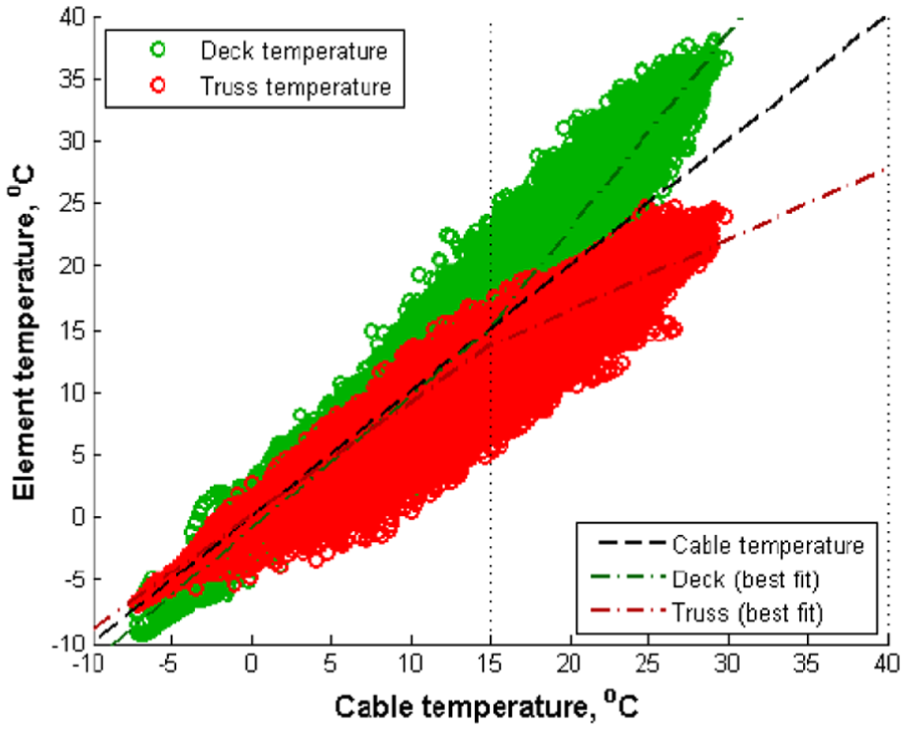
Assumed temperature relations between cable, shaded and lighted groups for Tamar bridge FE model and associated monitored data.
Thus, the relation between the temperatures of the shaded, lighted and cable groups is
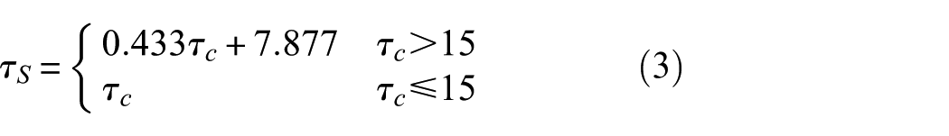
where
It must be stressed that the linear relations of equations (3) and (4) will only be applied when
Third, the effects of traffic load are also detailed. The traffic is assumed as a set of distributed mass points, evenly spread longitudinally across the bridge deck, and asymmetrically in the lateral direction. The average number of vehicles on the bridge in the tolled direction can be assumed as approximately 1/43rd of the available half-hourly count. Hence, traffic effects were monitored as a function of a half-hourly total mass
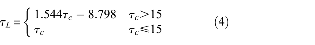
Finally, and gathering all the above-mentioned information, the simulations of the FE model have been performed in a Latin hypercube space, where values of temperature, traffic mass, and structural parameters were uniformly generated and the corresponding natural frequencies/displacements stored. A flowchart of the whole process is shown in Figure 7. First, a single modal analysis was run with default values of structural parameters and without traffic or temperature loading. In the second phase, multiple analyses were run for each combination of the input dataset
Simulation flowchart.
Parameter identification and discrepancy function prediction
MBA input dataset
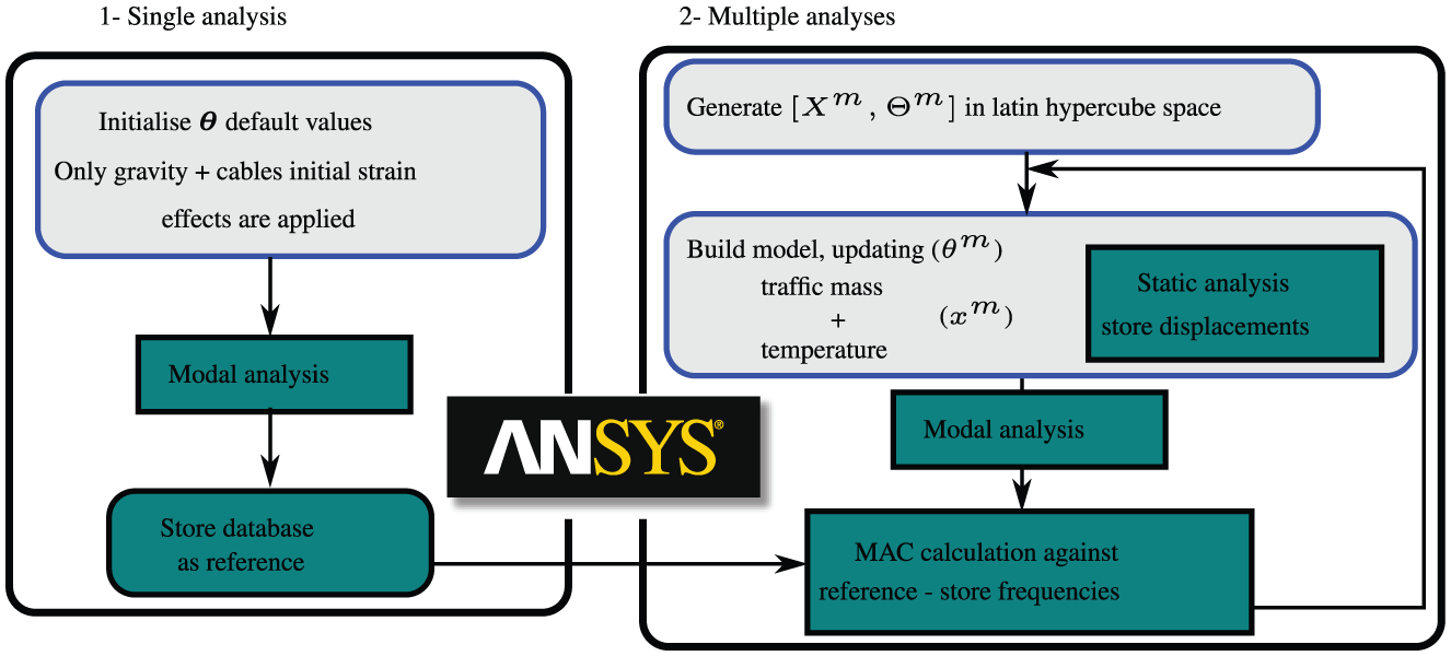
Table 2 presents a summary of all the MBA input data, and the to-be-identified structural parameters
MBA input dataset for Tamar bridge.
In order to sample the likelihood PDF with the MH algorithm, four Markov chains have been generated, with a standard multivariate normal distribution set as the proposal distribution. Trace plots of accepted samples are shown in Figure 8, and their acceptance ratio was 39%.
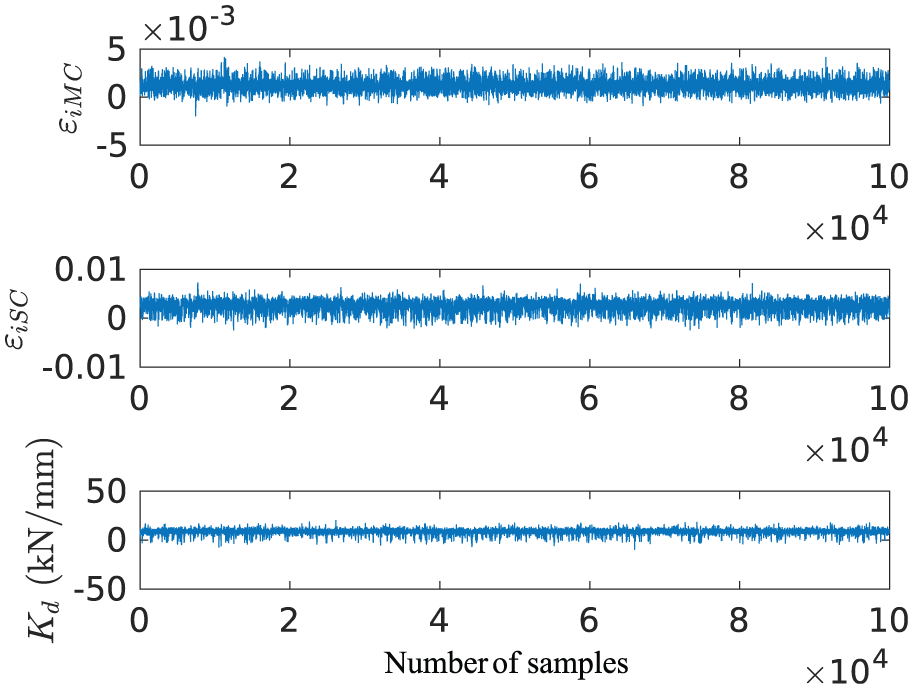
Trace plot of identified structural parameters.
Prediction of model discrepancy
Beforehand, it is important to predict a discrepancy function, whose information can be used to update the model, or added to the model output to compensate for inevitable modelling inadequacies. In the current section, some of the obtained discrepancy function predictions will be presented and commented. Since the outputs depend of temperature/traffic and mrGps are used for visualisation, the results assume the form of three-dimensional (3D) statistical response surfaces, that is, a mean 3D surface and a prediction interval cloud. However, for the sake of clarity, the prediction intervals surrounding the mean surface have been omitted. Finally, it is important to mention that when the predictions of the model agree more closely to the monitored data, for example, because the model has been fine-tuned and updated continuously, the closer the discrepancy function will be to a zero-mean uncorrelated Gaussian.
A first example of the mean discrepancy function of the natural frequencies of the Tamar bridge is shown in Figure 9. The first thing to observe is that none of the mean surfaces is close to zero, and all display a correlated behaviour. As noted before, wind also affects the natural frequencies of the Tamar bridge, so it is plausible to assume that the visible correlation is due to wind. Second, some patterns are visible in the lateral sway modes in Figure 9(a) and (d), where the discrepancy increases smoothly with traffic mass up to a localised peak at 1400 tonnes. Note that the same peak occurs, irrespective of temperature, which indicates that it depends only of the modelled traffic effects and predominantly during rushing hours. Thus, it is reasonable to assume that it occurs because our model does not consider traffic from the Plymouth to Saltash direction.
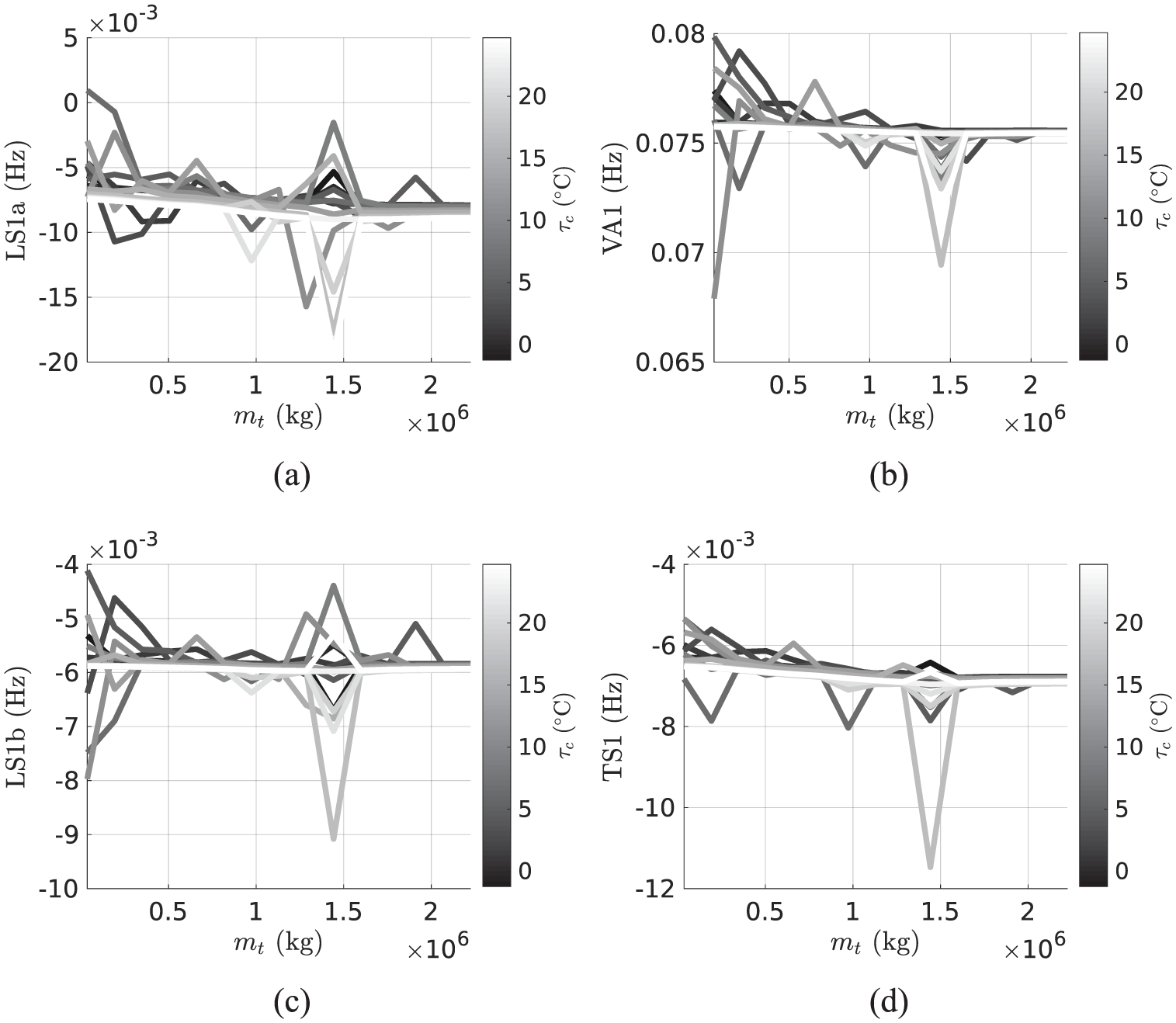
Prediction of the Tamar bridge natural frequency (a) LS1a, (b) VA1, (c) LS1b and (d) TS1 discrepancy function for varying temperature (grayscale lines) and traffic (abscissa) conditions.
Summarily, the results highlight the limitations of not considering a two-way traffic model and assuming an asymmetric distribution of traffic mass. Equipped with this information, an analyst could integrate it in its model predictions or carry out further updates.
Other example is shown in Figure 10, where the model discrepancy of the mid-span displacements is being predicted by the MBA. The results indicate a better performance, since the shown surface resembles a zero mean uncorrelated Gaussian, particularly visible for the displacement in the lateral North direction.
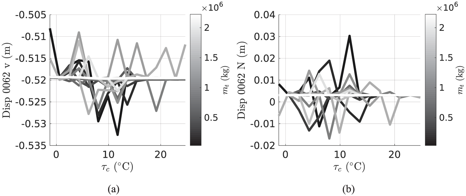
Prediction of the Tamar bridge mid-span (a) vertical and (b) Northern displacement discrepancy function for varying temperature (abscissa) and traffic (grayscale lines) conditions.
A final example is shown in Figure 11. The shown plots are equivalent to Figure 9(c) and (d) but with temperature in the abscissa. The model discrepancy for the two modes, LS1b and TS1, exhibits a temperature/traffic interaction, since recurrent peaks occur at different temperatures and traffic values. It is important to always identify such patterns, and in which responses they become more proeminent, in order to ensure that the model predictions can be properly interpreted.
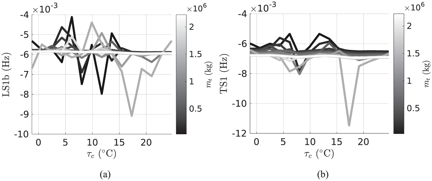
Prediction of the Tamar bridge natural frequency (a) LS1b and (b) TS1 discrepancy function for varying temperature (abscissa) and traffic (grayscale lines) conditions.
Validation of identified structural parameters
In this section, identified structural parameters are presented and validated. Whereas the results of the previous section are useful for model updating, identifying the true value of structural parameters is essential for damage detection or reliability analyses. It should be noted that compared to the hierarchical Bayes from Behmanesh et al., the MBA is unable to capture the inherent variability of structural parameters. Therefore, note that the variance shown in the following results is associated with the estimation uncertainty of the parameters.
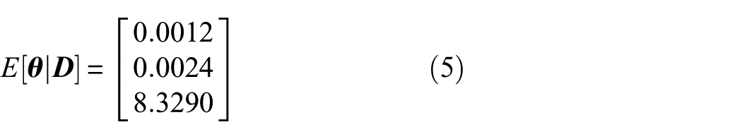
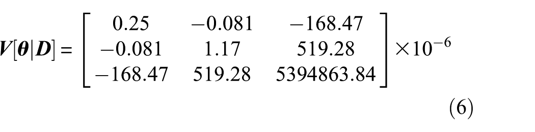
Sample histograms of the prior likelihood are displayed in Figure 12, and moments of the posterior distribution are shown in equations (5) and (6). Since an uninformative prior has been assumed, the posterior distribution and the maximum a posteriori (MAP) are proportional/equivalent to the values obtained from the likelihood
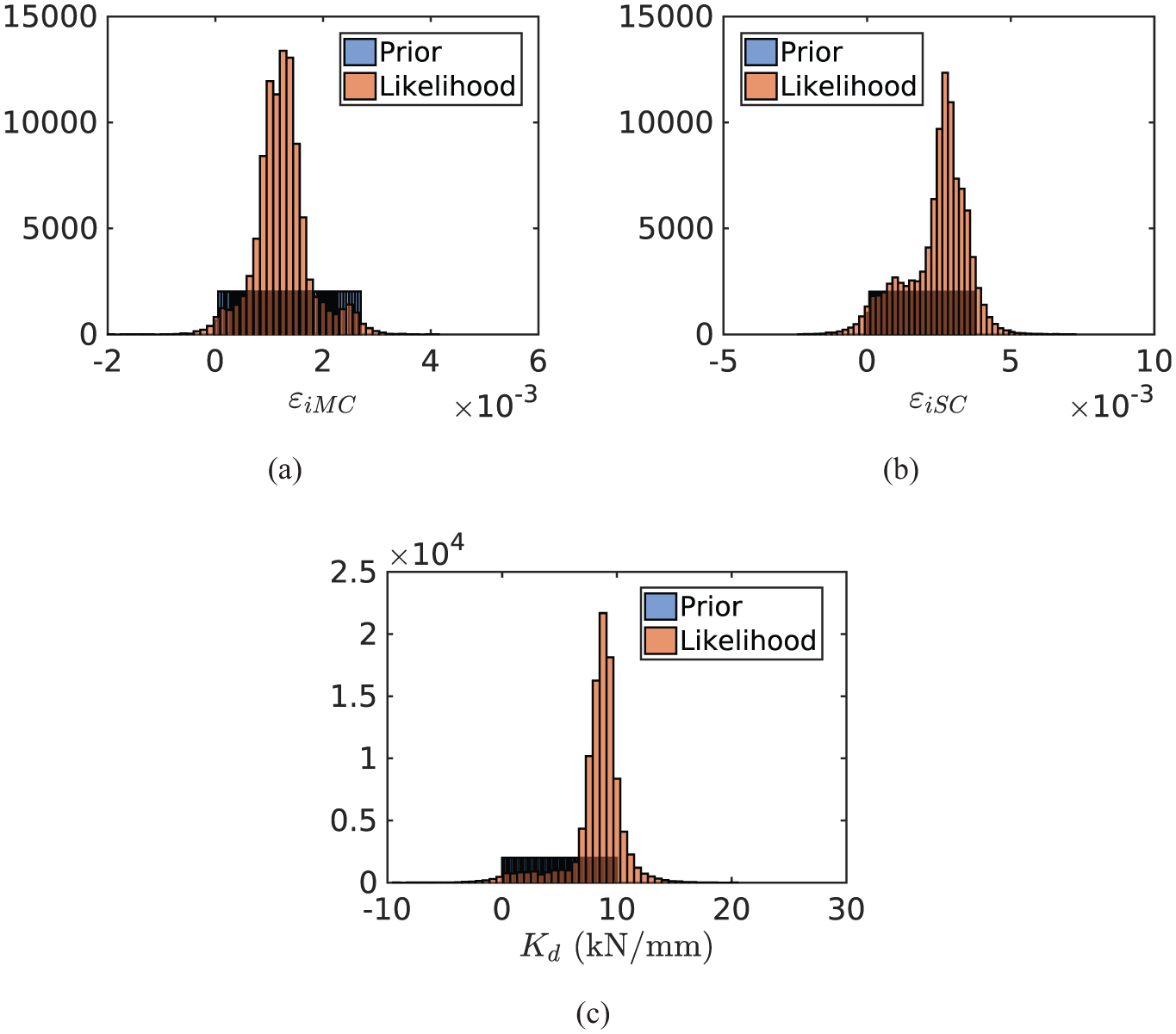
Inference of structural parameters: (a) main and (b) sway cables initial strain and (c) stiffness of thermal expansion gap.
Subsequently, validation of the identification of the stay cables and the thermal expansion gap will be presented. Opportunely, expeditions and other estimates are available from past literature. The only exception are the main cables, which have never been monitored, and since its strains vary along its length, their results will be ommited.
The above estimates shall now be compared against an st-id confidence interval reported by Laory et al. 44 and Goulet. 45 An estimate of the cables internal forces was obtained based on the initial strain MAP and the FE model predictions for each cable. Results are displayed in Table 3. For the stay cable forces, there is a reasonable agreement between the two methodologies, since the MBA MAP falls near the upper limits of the model falsification (MF) confidence interval. However, for the stiffness of the thermal expansion gap, the MBA estimate is considerably less than the MF interval. A high value of this parameter would indicate that the bridge deck is prone to develop cracks. In order to investigate which estimate is closer to the true friction value, and to further analyse the stay cables behaviour, a comparison against monitored data will be detailed next.
Identification of cable forces, stiffness of thermal expansion gap and comparison against model falsification.
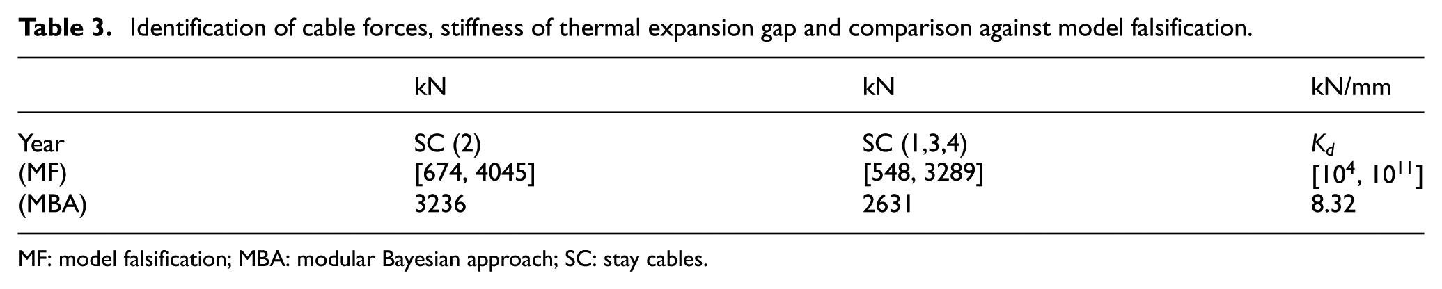
MF: model falsification; MBA: modular Bayesian approach; SC: stay cables.
The predicted stay cable forces are plotted along with monitored forces from existent strain gauge load cells, as shown in Figure 13. It is also important to stress that these monitored forces have not been used to estimate the posterior PDF. Both histograms have been normalised in the coordinate axis by an estimate of probability density.
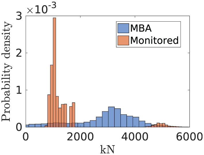
Tamar bridge histogram of monitored, during January–July 2008, and identified stay cable forces. The right isolated peak represents the monitored P3S cable.
First, it can be seen that the P3S cable has three to four times larger forces, and as reported in Koo et al., 46 has a stronger dependency on temperature, than other stay cables. It is not certain why such behaviour occurs. Second, it can be observed that the posterior obtained by the MBA falls between the P3S and the other cables histograms. Two reasons might aid to clarify this result:
Since the parameter is assumed constant across all cables, its posterior distribution falls between the two other histograms, acting as an average value.
The offset might occur because the parameter represents an initial strain, that is, the strain relative to when the bridge cables have been installed on the bridge, and not relative to the strain existent when the strain gauge load cells have been installed.
Note that point number 1 assumes that the P3S cables force is genuine, in which case the posterior distribution would have to be shifted towards lower values (since there are much more cables in the lower cable forces region). Thus, it is more plausible to believe that point 2 is the underlying reason for the posterior position, and that the values it indicates are closer to the true structural behaviour of the cables.
Finally, Battista et al. 47 recorded temperature and extension data in the thermal expansion gap, starting 2 months after the timeframe of data used for the MBA identification, that is, in July 2010. Results from Battista’s work revealed that the gap extension against temperature is perfectly adjusted to a linear relation (see Figure 15 of the above work for clarification) and does not indicate any relevant frictional force. Hence, a lower value of stiffness, such as the one identified by the MBA, suggests a better agreement with in situ tests.
Conclusion
In this work, the MBA has been applied for st-id of the Tamar long suspension bridge. The methodology has been expanded to identify multiple structural parameters, including the bridge’s cables initial strain and the stiffness of its thermal expansion gap. A detailed FE model of the bridge, on which environmental and operational effects were considered, has been calibrated and its performance has been assessed by a predicted model discrepancy.
Results suggest that
The developed methodology is able to identify multiple parameters using the MH and a multi-dimensional Monte Carlo integration.
Compared against work from previous authors, the MBA provides an identification which agrees more reasonably with monitored data, particularly for the friction of the thermal expansion gap. This has been validated with in situ tests.
The current analysis is conditioned by the ability of its user to model environmental/operational effects. However, in contrast with other Bayesian methodologies, it is capable of performing st-id on large-scale infrastructure, highlighting trends and patterns of model discrepancy.
In general, the Tamar bridge FE model performs better at predicting the mid-span displacements than natural frequencies. In addition, the limitations of the developed traffic model and its interactions with temperature have been presented and discussed.
The calibrated FE model can be used as a reference baseline, for further investigations/health assessments, for example, damage detection.
In conclusion, the application of the MBA for st-id for large-scale civil structures has been comprehensively detailed in this work, and although this study presented some limitations, the authors believe that it is a reliable tool for the SHM community.
Footnotes
Acknowledgements
The main author gratefully acknowledges the computing resources provided by the Cluster of Workstations operated by the Centre for Scientific Computing of the University of Warwick. The authors would like to thank the journal reviewers for their valuable comments, which have greatly improved the manuscript.
Declaration of conflicting interests
The author(s) declared no potential conflicts of interest with respect to the research, authorship and/or publication of this article.
Funding
This work was supported by the Engineering and Physical Sciences Research Council (EPSRC) reference number EP/N509796 and partially funded by the British Council (Grant ID: 217544274).