Sage Journals: Discover world-class research

Abstract

Data generated by high-throughput screening (HTS) technologies are prone to spatial bias. Traditionally, bias correction methods used in HTS assume either a simple additive or, more recently, a simple multiplicative spatial bias model. These models do not, however, always provide an accurate correction of measurements in wells located at the intersection of rows and columns affected by spatial bias. The measurements in these wells depend on the nature of interaction between the involved biases. Here, we propose two novel additive and two novel multiplicative spatial bias models accounting for different types of bias interactions. We describe a statistical procedure that allows for detecting and removing different types of additive and multiplicative spatial biases from multiwell plates. We show how this procedure can be applied by analyzing data generated by the four HTS technologies (homogeneous, microorganism, cell-based, and gene expression HTS), the three high-content screening (HCS) technologies (area, intensity, and cell-count HCS), and the only small-molecule microarray technology available in the ChemBank small-molecule screening database. The proposed methods are included in the AssayCorrector program, implemented in R, and available on CRAN.

Keywords

Anderson–Darling test Cramer–von Mises test data correction high-content screening high-throughput screening partial mean polish small-molecule microarray spatial bias

Introduction

The amount of data generated by high-throughput screening (HTS) technologies that can be used to identify active compounds, such as small molecules, small interfering RNAs (siRNAs), or gene expression profiles, has exploded in recent years.^1,2 This breakthrough has been triggered by a significant drop in the cost of screening technologies. Data generated by HTS technologies are, however, often subject to different types of spatial bias, which negatively influence the outcomes of HTS campaigns.^3,4 Spatial bias is usually caused by environmental (e.g., irregular changes in the temperature, incubation time, lighting, and air flow) or technical (e.g., pipette and reader effects) factors.^5–7 Plate-specific spatial bias (i.e., plate-specific systematic error) is evident as an under- or overestimation of measurements in certain rows and columns of a given plate. Often, spatial bias affects the edges of a given plate, causing the so-called edge effect. The intersection of rows and columns affected by spatial biases can be of particular interest because the resulting activity measurements depend on the interaction between these biases.

Plate-specific spatial bias in HTS has been traditionally assumed to fit the following additive model⁸ (Equation 1):

{x^{'}}_{i j p} = x_{i j p} + r_{i p} + c_{j p} + ε_{i j p},

where ${x^{'}}_{i j p}$ is the biased measurement value in well (i,j) of plate p, $x_{i j p}$ the unbiased measurement value in this well, $r_{i p}$ is the bias affecting row i of plate p, C_jp is the bias affecting column j of plate p, and ε_ijp is the random error in well (i,j) of plate p.

Recent studies have suggested that plate-specific spatial bias can also be of the multiplicative kind⁹ (Equation 2):

{x^{'}}_{i j p} = x_{i j p} \times r_{i p} \times c_{j p} + ε_{i j p} .

Correction methods based on different statistical procedures have been developed to remove systematic error using either the classical additive or classical multiplicative spatial bias models. For instance, the additive bias model was used in the following bias correction techniques: B-score,¹⁰ R-score,¹¹ additive partial mean polish (aPMP),¹² and SPAWN.¹³ The diffusion model³ and the multiplicative PMP (mPMP) method⁹ are among a few multiplicative bias models. The issue of correcting measurements located at the intersection of biased rows and columns has not, however, been addressed so far.

In this article, we introduce two additive and two multiplicative bias models, proposing different treatments of measurements located at the intersections of biased rows and columns, and a new statistical procedure, based on the use of the Anderson–Darling (AD)¹⁴ or Cramer–von Mises (CVM)¹⁵ goodness-of-fit tests, which allows one to select the most appropriate spatial bias model for a given plate. This procedure includes modeling bias effects by using traditional additive and multiplicative bias equations (Equations 1–2) as well as the arithmetic and geometric means to describe possible interactions between row and column spatial biases. The Mann–Whitney U test is used in our procedure to identify rows and columns of a given plate that are affected by spatial bias. A new variant of the PMP algorithm^9,12 will be used to remove systematic error from biased plate measurements. The discussed statistical procedure will be applied to analyze experimental data generated by high-throughput (HTS), high-content (HCS), and small-molecule microarray (SMM) screening technologies, publicly available at ChemBank.¹⁶

Methods

In this section, we present the statistical methods we propose to carry out to detect and remove additive and multiplicative spatial biases from multiwell plates used in screening technologies. Spatial bias present in rows and columns of a given plate is first detected using the nonparametric Mann–Whitney U test. Then, the most appropriate additive or multiplicative bias model will be determined, and the corresponding bias removal algorithm will be carried out. Six spatial bias models will be described here, including four new models. The CVM and AD tests will be used to assess the goodness-of-fit between raw and corrected screening measurements.

Spatial Bias Detection in Multiwell Plates

The nonparametric Mann–Whitney U test was applied to identify rows and columns of a given plate that are affected by spatial bias. In contrast to the t-test, which was used for example in Dragiev et al.,¹² the Mann–Whitney U test makes no assumptions about the underlying distribution (e.g., normality), is at least 86.4% asymptotically as efficient as the t-test,¹⁷ and is robust to outlying observations.

Our spatial bias detection algorithm proceeds by assessing the difference in the compound activity values between a given row or column (Sample 1) and the rest of the plate’s measurements (Sample 2). Once all rows and columns have been assessed in turn, the row or column with the smallest statistically significant p-value is added to the set of biased locations (i.e., rows and columns). The process continues either until convergence (i.e., until no more significant p-values are found) or until a fixed proportion of rows and columns containing spatial bias has been found.

Correction of Plate-Specific Bias

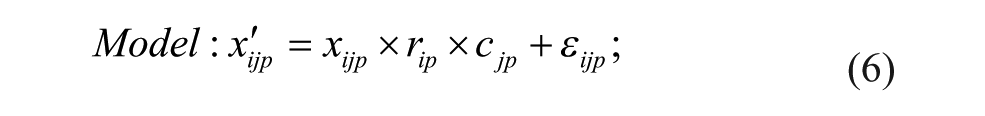
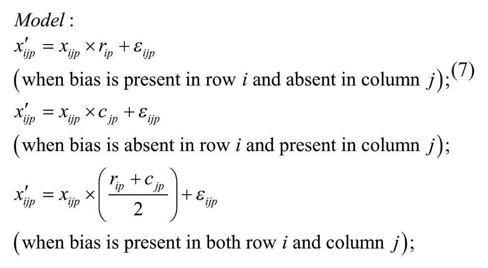
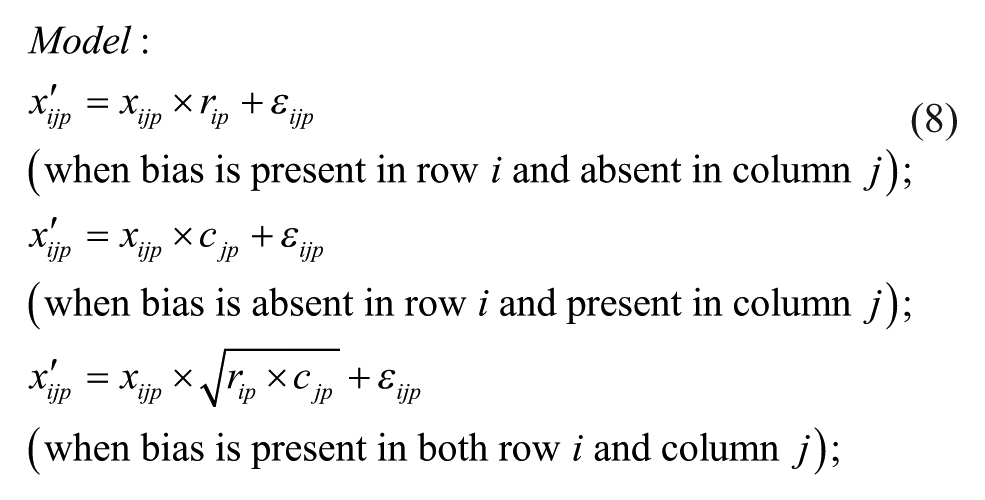
Plate-specific biases affecting rows and columns of a given plate p with m rows and n columns can fit either the additive (Models 1–3, below) or multiplicative (Models 4–6, below) bias model, which can be described by the following equations (with 1 ≤ i ≤ m and 1 ≤ j ≤ n).

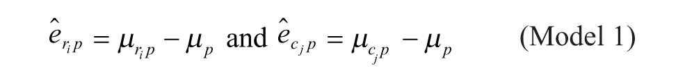
Model 1: Additive Model

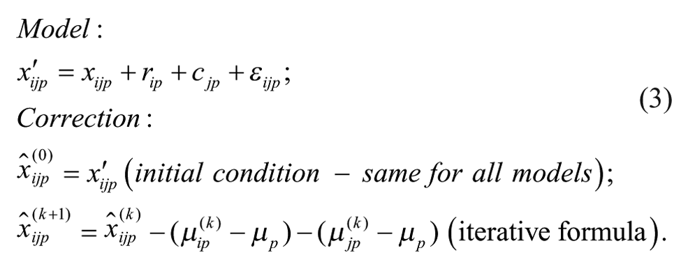
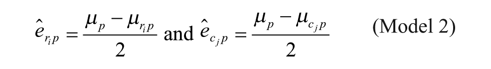
\begin{array}{l} M o d e l : \\ {x^{'}}_{i j p} = x_{i j p} + r_{i p} + c_{j p} + ε_{i j p}; \\ C o r r e c t i o n : \\ {\hat{x}}_{i j p}^{(0)} = {x^{'}}_{i j p} (i n i t i a l c o n d i t i o n - s a m e f o r a l l m o d e l s); \\ {\hat{x}}_{i j p}^{(k + 1)} = {\hat{x}}_{i j p}^{(k)} - (μ_{i p}^{(k)} - μ_{p}) - (μ_{j p}^{(k)} - μ_{p}) (iterative formula) . \end{array}

Model 2: Additive Model with Arithmetic Mean at the Intersection

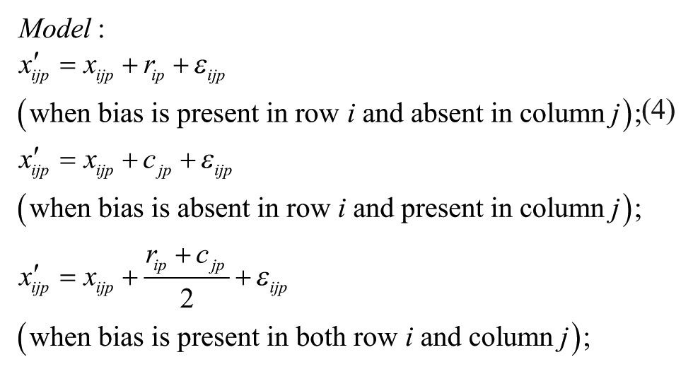
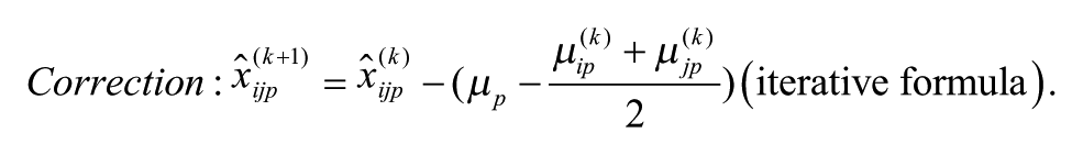
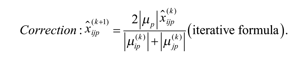
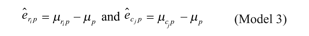
\begin{array}{l} M o d e l : \\ {x^{'}}_{i j p} = x_{i j p} + r_{i p} + ε_{i j p} \\ (when bias is present in row i and absent in column j); \\ {x^{'}}_{i j p} = x_{i j p} + c_{j p} + ε_{i j p} \\ (when bias is absent in row i and present in column j); \\ {x^{'}}_{i j p} = x_{i j p} + \frac{r_{i p} + c_{j p}}{2} + ε_{i j p} \\ (when bias is present in both row i and column j); \end{array}

C o r r e c t i o n : {\hat{x}}_{i j p}^{(k + 1)} = {\hat{x}}_{i j p}^{(k)} - (μ_{p} - \frac{μ_{i p}^{(k)} + μ_{j p}^{(k)}}{2}) (iterative formula) .

Model 3: Additive Model with Multiplicative Interaction of Biases at the Intersection

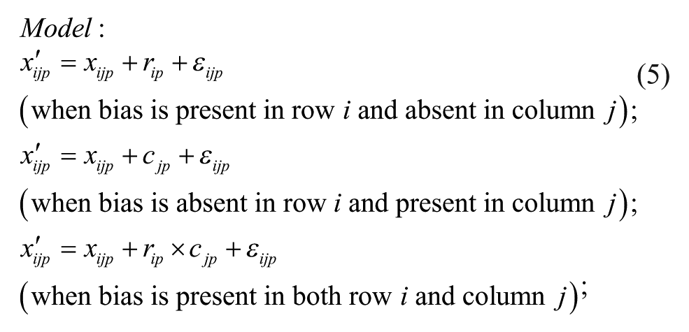
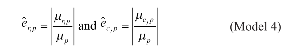
\begin{array}{l} M o d e l : \\ {x^{'}}_{i j p} = x_{i j p} + r_{i p} + ε_{i j p} \\ (when bias is present in row i and absent in column j); \\ {x^{'}}_{i j p} = x_{i j p} + c_{j p} + ε_{i j p} \\ (when bias is absent in row i and present in column j); \\ {x^{'}}_{i j p} = x_{i j p} + r_{i p} \times c_{j p} + ε_{i j p} \\ (when bias is present in both row i and column j); \end{array}

C o r r e c t i o n : {\hat{x}}_{i j p}^{(k + 1)} = {\hat{x}}_{i j p}^{(k)} - (μ_{i p}^{(k)} - μ_{p}) (μ_{j p}^{(k)} - μ_{p}) (iterative formula) .

Model 4: Multiplicative Model

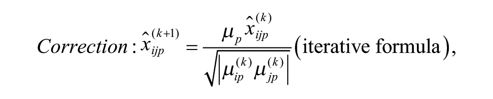
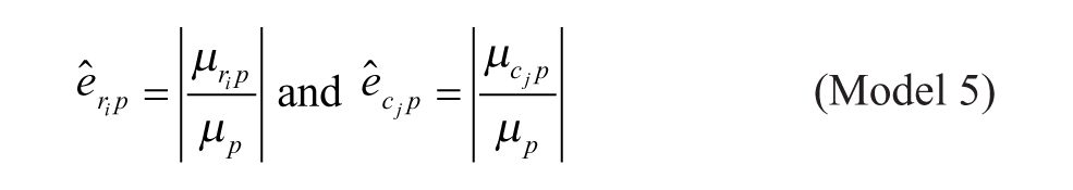
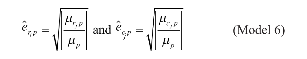
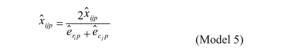
M o d e l : {x^{'}}_{i j p} = x_{i j p} \times r_{i p} \times c_{j p} + ε_{i j p};

C o r r e c t i o n : {\hat{x}}_{i j p}^{(k + 1)} = \frac{μ_{p}^{2} {\hat{x}}_{i j p}^{(k)}}{| μ_{i p}^{(k)} μ_{j p}^{(k)} |} (iterative formula) .

Model 5: Multiplicative Model with Arithmetic Mean at the Intersection

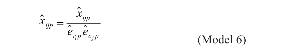
\begin{array}{l} M o d e l : \\ {x^{'}}_{i j p} = x_{i j p} \times r_{i p} + ε_{i j p} \\ (when bias is present in row i and absent in column j); \\ {x^{'}}_{i j p} = x_{i j p} \times c_{j p} + ε_{i j p} \\ (when bias is absent in row i and present in column j); \\ {x^{'}}_{i j p} = x_{i j p} \times (\frac{r_{i p} + c_{j p}}{2}) + ε_{i j p} \\ (when bias is present in both row i and column j); \end{array}

C o r r e c t i o n : {\hat{x}}_{i j p}^{(k + 1)} = \frac{2 | μ_{p} | {\hat{x}}_{i j p}^{(k)}}{| μ_{i p}^{(k)} | + | μ_{j p}^{(k)} |} (iterative formula) .

Model 6: Multiplicative Model with Geometric Mean at the Intersection

\begin{array}{l} M o d e l : \\ {x^{'}}_{i j p} = x_{i j p} \times r_{i p} + ε_{i j p} \\ (when bias is present in row i and absent in column j); \\ {x^{'}}_{i j p} = x_{i j p} \times c_{j p} + ε_{i j p} \\ (when bias is absent in row i and present in column j); \\ {x^{'}}_{i j p} = x_{i j p} \times \sqrt{r_{i p} \times c_{j p}} + ε_{i j p} \\ (when bias is present in both row i and column j); \end{array}

C o r r e c t i o n : {\hat{x}}_{i j p}^{(k + 1)} = \frac{μ_{p} {\hat{x}}_{i j p}^{(k)}}{\sqrt{| μ_{i p}^{(k)} μ_{j p}^{(k)} |}} (iterative formula),

where ${x^{'}}_{i j p}$ is the biased (i.e., observed) raw measurement in well (i,j) of plate p, x_ijp is the unbiased activity measurement in well (i,j) of plate p, ${\hat{x}}_{i j p}$ is the estimated measurement in well (i,j) of plate p, k is the iteration number, r_ip is the value of systematic error (i.e., spatial bias) affecting row i of plate p, c_jp is the value of systematic error affecting column j of plate p, $μ_{p}$ is the mean of unbiased measurements of plate p, µ_ip is the mean of measurements in row i of plate p, µ_jp is the mean of measurements in column j of plate p, and ε_ijp is the random error affecting well (i,j) of plate p. The random error ε_ijp is assumed to be small compared to the values of spatial biases c_jp and r_ip. The impact of random errors on the hit selection process can be minimized by using compounds’ replicates.^4,8 In the additive models (Models 1–3), unbiased rows and columns have r_ip = 0 and c_jp = 0, respectively, whereas in the multiplicative models (Models 4–6), unbiased rows and columns have r_ip = 1 and c_jp = 1, respectively.

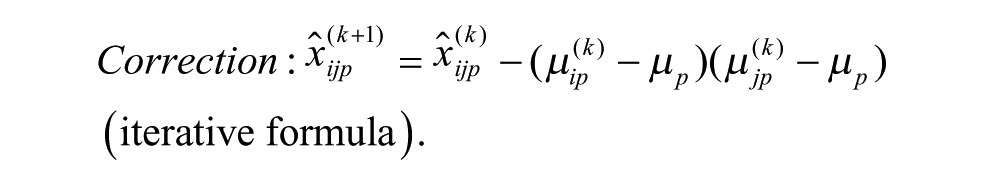
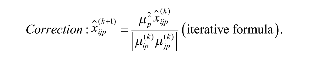
Model 1 is the traditional additive model, which is assumed in many bias correction methods.^10,12,13 Model 2 is an additive model that assumes that the row and column biases at the intersections are combined through their arithmetic mean. Model 3 is an additive model that assumes that the row and column biases at the intersections interact in a multiplicative fashion. Model 4 is a recently introduced basic multiplicative bias model. Model 5 is a multiplicative model that assumes that the intersection effects of row and column biases are combined through their arithmetic mean. Model 6 is a multiplicative model that assumes that the row and column biases at the intersection are combined through their geometric mean. Models 2 and 3 can be viewed as extensions of the additive PMP model (Model 1), whereas Models 5 and 6 can be viewed as extensions of the multiplicative PMP model (Model 4). PMP algorithms^9,12 are variations of Tukey’s median polish,¹⁸ which iteratively removes spatial bias from the rows and columns affected.

Model Selection for Removing Plate-Specific Spatial Bias

In this section, we present a data-processing protocol that can be used to identify the most appropriate spatial bias model for a given plate. If the presence of spatial bias in a given plate has been detected using the Mann–Whitney U test, then we first partition all wells of the plate into (1) wells with no bias detected and (2) wells located in biased rows and columns. Control wells should be excluded from all computations. Wells affected by spatial bias can then be corrected using the six iterative methods (Models 1–6) discussed above. Our procedure generates seven sets of data: a set of unbiased wells, and six sets of biased wells corrected by each of the six methods. The AD or CVM test can then be used on the set of unbiased wells and on each of the six corrected sets of wells to assess goodness-of-fit of the corrections performed. The resulting p-values can then be used to determine the most appropriate bias model (among Models 1–6) for the data at hand. In this work, the significance level α was set to 0.01 for all three statistical tests being performed (the Mann–Whitney U test, AD test, and CVM test). Both the AD and CVM tests can be used in the algorithm below, but the AD test is preferred due to its higher power.²¹

Our algorithm proceeds as follows:

i. Perform the Mann–Whitney U test on each individual plate of the assay (i.e., plate-wise correction) to identify biased rows and columns.

For each plate containing biased rows and/or columns, perform:

ii. Apply each of the six additive and multiplicative PMP algorithms corresponding to Models 1–6, as discussed in this section (see the related iterative formulas 3 to 8).

iii. Apply the AD or CVM two-sample test on the corrected plates after the application of the six versions of the PMP algorithm. Compute the corresponding p-values (three additive and three multiplicative).

iv. If all additive and multiplicative p-values are higher than the selected significance level α, the bias model for this plate is the model with the highest p-value (low confidence).

v. If all additive p-values are lower than the selected significance level α, and all multiplicative p-values are higher than a, the bias model for this plate is multiplicative (high confidence).

vi. If all multiplicative p-values are lower than the selected significance level α, and all additive p-values are higher than α, the bias model for this plate is additive (high confidence).

vii. If none of the conditions specified in Steps iv to vi apply, then the bias model is undefined.

viii. If the bias model has been identified (i.e., it is not undefined), then correct the plate measurements using the corresponding bias correction procedure.

Traditional and Modified Partial Mean Polish Algorithms

In this section, we present the details of the aPMP and mPMP algorithms corresponding to Models 1 to 6, discussed above. The main advantage of these algorithms compared to the popular B-score method of Brideau et al.¹⁰ is that they do not reduce the original measurements to residuals and do not modify the unbiased measurements.

Our generalized PMP algorithm proceeds as follows:

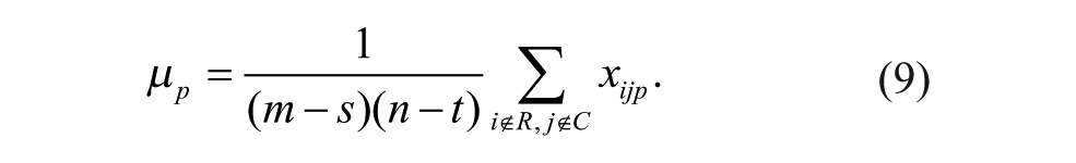
Let $R = {r_{1}, r_{2}, \dots, r_{s} | 0 \leq s < m}$ and $C = {c_{1}, c_{2}, \dots, c_{t} | 0 \leq t < n}$ be the sets of biased rows and columns of plate $p (m \times n)$ , respectively. Calculate the mean, µ_p, of all unbiased measurements of p:

μ_{p} = \frac{1}{(m - s) (n - t)} \sum_{i \notin R, j \notin C} x_{i j p} .

For each biased row i : 1 ≤ i ≤ s_n, calculate the mean value, $μ_{r_{i} p}$ , of row r_i: $μ_{r_{i} p} = \frac{1}{n} \sum_{j = 1}^{n} x_{r_{i} j p}$ , and the estimate of the row bias, ${\hat{e}}_{r_{i} p}$ . For each biased column $j : 1 \leq j \leq t$ , calculate the mean value, $μ_{c_{j} p}$ of column c_j: $μ_{c_{j} p} = \frac{1}{m} \sum_{i = 1}^{m} x_{i c_{j} p}$ , and the estimate of the column error, ${\hat{e}}_{c_{j} p}$ . Use the following equations to calculate the error estimates:

{\hat{e}}_{r_{i} p} = μ_{r_{i} p} - μ_{p} and {\hat{e}}_{c_{j} p} = μ_{c_{j} p} - μ_{p}

(Model 1)

{\hat{e}}_{r_{i} p} = \frac{μ_{p} - μ_{r_{i} p}}{2} and {\hat{e}}_{c_{j} p} = \frac{μ_{p} - μ_{c_{j} p}}{2}

(Model 2)

{\hat{e}}_{r_{i} p} = μ_{r_{i} p} - μ_{p} and {\hat{e}}_{c_{j} p} = μ_{c_{j} p} - μ_{p}

(Model 3)

{\hat{e}}_{r_{i} p} = | \frac{μ_{r_{i} p}}{μ_{p}} | and {\hat{e}}_{c_{j} p} = | \frac{μ_{c_{j} p}}{μ_{p}} |

(Model 4)

{\hat{e}}_{r_{i} p} = | \frac{μ_{r_{i} p}}{μ_{p}} | and {\hat{e}}_{c_{j} p} = | \frac{μ_{c_{j} p}}{μ_{p}} |

(Model 5)

{\hat{e}}_{r_{i} p} = \sqrt{| \frac{μ_{r_{i} p}}{μ_{p}} |} and {\hat{e}}_{c j p} = \sqrt{| \frac{μ_{c_{j} p}}{μ_{p}} |}

(Model 6)

For all rows and columns affected by spatial bias, iteratively adjust their measurements using the error estimates determined in Step 2. In other words, for all $i : 1 \leq i \leq s$ and $j : 1 \leq j \leq t$ , proceed as follows:

{\hat{x}}_{i j p} = {\hat{x}}_{i j p} - ({\hat{e}}_{r_{i} p} + {\hat{e}}_{c_{j} p})

(Model 1)

{\hat{x}}_{i j p} = {\hat{x}}_{i j p} - ({\hat{e}}_{r_{i} p} + {\hat{e}}_{c_{j} p})

(Model 2)

{\hat{x}}_{i j p} = {\hat{x}}_{i j p} - {\hat{e}}_{r_{i} p} {\hat{e}}_{c_{j} p}

(Model 3)

{\hat{x}}_{i j p} = \frac{{\hat{x}}_{i j p}}{{\hat{e}}_{r_{i} p} {\hat{e}}_{c_{j} p}}

(Model 4)

{\hat{x}}_{i j p} = \frac{2 {\hat{x}}_{i j p}}{{\hat{e}}_{r_{i} p} + {\hat{e}}_{c_{j} p}}

(Model 5)

{\hat{x}}_{i j p} = \frac{{\hat{x}}_{i j p}}{{\hat{e}}_{r_{i} p} {\hat{e}}_{c_{j} p}}

(Model 6)

If $\sum_{i = 1}^{s} | {\hat{e}}_{r_{i} p} | \sum_{j = 1}^{t} | {\hat{e}}_{c_{j} p} | > ε$ , then go to Step 2; otherwise, stop the algorithm.

where ε is a small, fixed, positive threshold.

Choice of Statistical Test to Determine the Bias Model

Two statistical tests, used in Step iii of the above-presented bias correction protocol, were examined to assess the goodness-of-fit between raw and corrected measurements: the CVM and AD tests. The AD test is based on a quadratic empirical distribution function (EDF) statistic. Importantly, the AD test has been shown to be the most powerful among the EDF tests.¹⁹ The CVM test is a special case of AD that puts less weight on the tails of the distribution. It has been shown that the power of the AD test is higher than that of the Kolmogorov–Smirnov,²⁰ probability-plot, L moments, and chi-square (χ²) tests.²¹ Moreover, the AD test is generally more powerful than the CVM test.²² These conclusions mirror those formulated by Stephens.²³

Simulations

We conducted a simulation study to estimate the efficiency of our new additive and multiplicative bias models (Models 1–6, above) and the corresponding versions of the PMP algorithm (see Fig. 1 ). We generated synthetic HTS data with known hits and plate-specific spatial biases to compare the performances of our new algorithm to those of the no-correction and B-score¹⁰ methods. It is worth noting that B-score remains the most popular bias correction method used in HTS. In our simulation study, we followed the data generation procedure initially described by Dragiev et al.¹² Precisely, we generated synthetic HTS data for 100 assays, each consisting of 100 plates of size (16×24), which is the most popular plate format in ChemBank,¹⁶ for every combination of parameters reported below. The values of nonhit compound measurements followed the standard normal distribution. Hit values were generated using the normal distribution with the following parameters: ~N(µ – 6SD, SD), where µ and SD were the mean and standard deviation of nonhit compounds, set to 0 and 1, respectively. Hit positions within plates were selected using rejection sampling with the following hit percentages: 0.5%, 1%, 2%, 3%, 4%, and 5%. Spatial bias was then added to selected rows and columns of the generated HTS plates using bias Models 1 to 6. In our simulations, at most 8 rows and 12 columns of each plate could be affected by bias. For every plate, the number of biased rows was sampled from a ~Geometric(p = 0.622) distribution, and the number of biased columns was sampled from a ~Geometric(p = 0.430) distribution. These parameters were estimated from experimental screening data consisting of 2441 non-empty plates of the 175 ChemBank assays considered in our work (see Suppl. Table 1 ). The maximum likelihood approach was applied to the distribution of the numbers of biased rows and columns in these assays (see Fig. 2 ) to get these parameters. The Mann–Whitney U test was used to detect the presence of spatial bias in the experimental ChemBank data.

Figure 1.

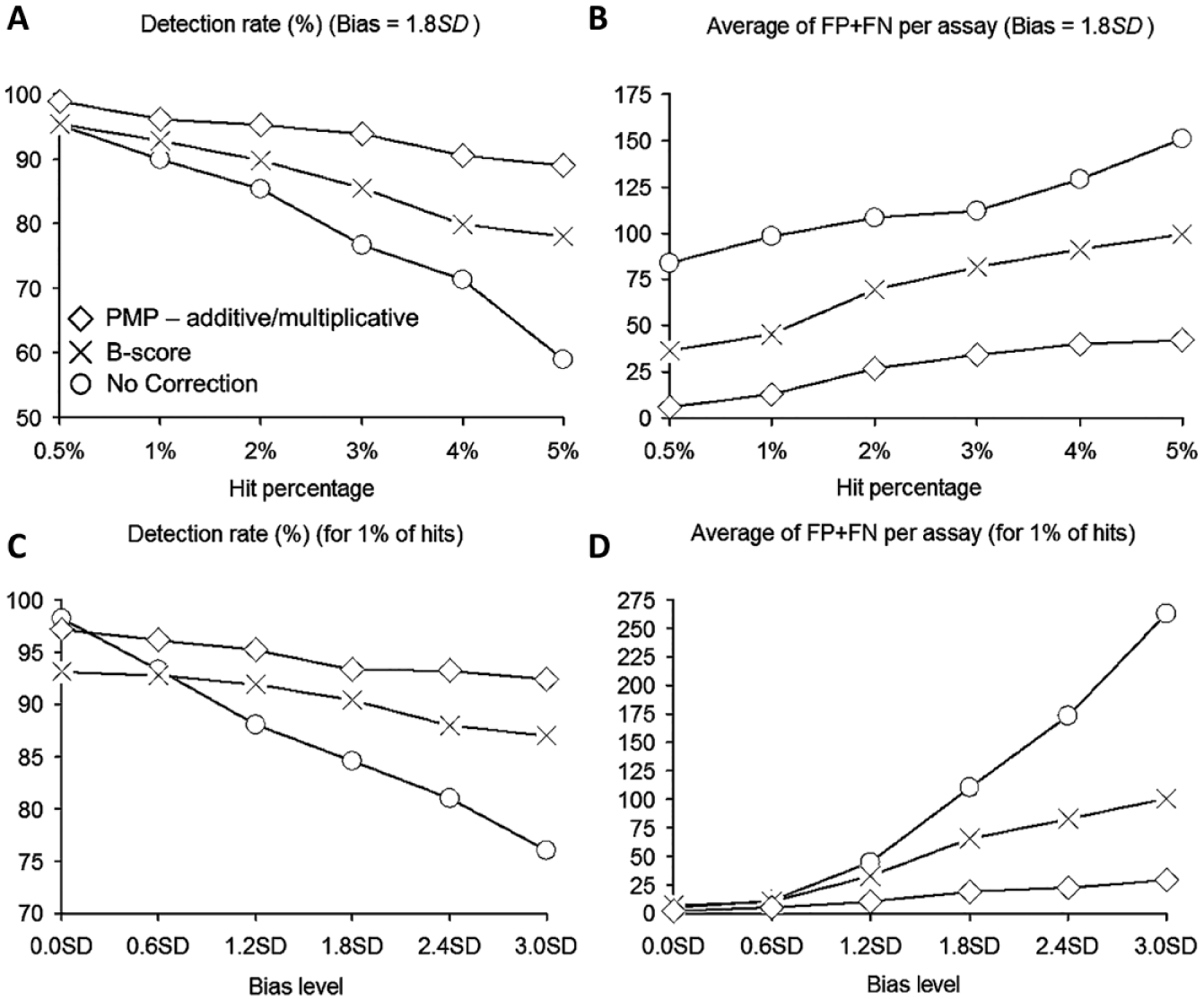
(A,C) Average true-positive rate, and (B,D) average total number of false-positive and false-negative hits per assay, obtained by using the no-correction, B-score, and partial mean polish (PMP) methods (based on Models 1–6, the nonparametric Mann–Whitney U test for bias detection, and the Anderson–Darling test for bias model selection). (A,B) The results obtained with a fixed bias level of 1.8 SD; (C,D) the results obtained with a fixed hit percentage of 1%.

Figure 2.

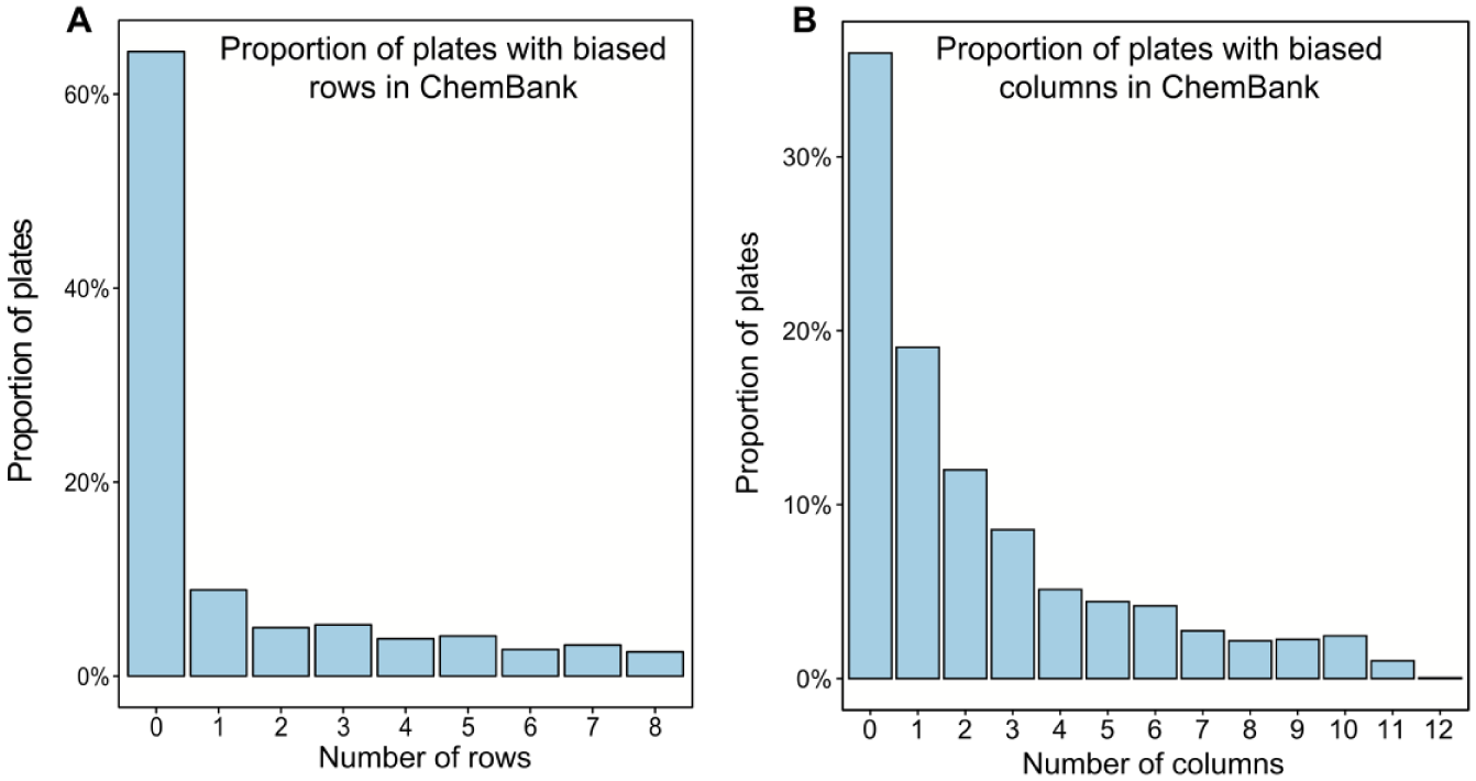
Proportion of plates with the indicated (A) number of rows affected by spatial bias and (B) number of columns affected by spatial bias. The nonparametric Mann–Whitney U test was used to detect the presence of spatial bias within each plate.

The bias model for each plate was selected from (1) undefined or no bias, (2) additive bias (Models 1 to 3), and (3) multiplicative bias (Models 4 to 6), with the following respective sampling probabilities: 0.274, 0.418, and 0.308, which were also estimating from the 2441 non-empty ChemBank plates considered here. In Models 1 to 6, the additive plate-specific biases were generated using the normal distribution with parameters ~N(0, C) and the multiplicative plate-specific biases using the normal distribution with parameters ~N(1, C), where parameter C was alternately set to 0, 0.6 SD, 1.2 SD, 1.8 SD, 2.4 SD, and 3 SD. Sample activity measurements affected by additive spatial bias were generated using Equations (3) to (5); and those affected by multiplicative spatial bias, using Equations (6) to (8). A random additive Gaussian noise (i.e., the parameter ε_ijp in Equations [3] to [8]), affecting both hit and nonhit activity measurements, was generated using the normal distribution with parameters ~N(0, 0.1SD). Our PMP algorithm correcting both additive and multiplicative spatial biases was used with the Mann–Whitney U test, which was applied to identify biased rows and columns within each plate, and the AD test, which was applied to select the most appropriate bias model (for more details, see the Methods section). The significance threshold α was set to 0.01 in both of these tests.

Following the data correction, the hit selection procedure was carried out using the µ_p – 3σ_p hit selection threshold, where µ_p and σ_p were the mean and standard deviation of the measurements of plate p. The methods’ performances were measured by using the hit recovery rate (i.e., true positive rate) and the total of false positives and false negatives they returned (see also Dragiev et al.¹²). Two simulations were conducted. In the first simulation (see Fig. 1A and 1B ), the bias level was set to 1.8 SD (fixed), whereas the hit percentage varied from 0% to 5%. In the second simulation (see Fig. 1C and 1D ), the hit percentage was set to 1% (fixed), whereas the noise level varied from 0 to 3 S.

The results of our simulations confirm that the bias correction methods should be used only when the presence of spatial bias was identified by a suitable statistical test. This is especially true for the B-score method. The obtained results suggest that the additive and multiplicative PMP algorithms, following Models 1 to 6 presented in the Methods section, provide the smallest total false-positive and false-negative hit counts as well as the best hit detection rate compared to the no-correction and B-score methods. When the hit percentage was varying from 0.5% to 5% and the bias level remained fixed at 1.8 SD ( Fig. 1A ), as well as when the bias magnitude was varying from 0.0 SD to 3.0 SD and the hit percentage remained fixed at 1% ( Fig. 1C ), the true-positive rate for all methods decreased with the increase in the hit percentage. When the hit percentage was varying from 0.5% to 5% and the bias level remained constant at 1.8 SD ( Fig. 1B ), the total count of false positives and false negatives was increasing for all methods. The PMP algorithm yielded the lowest average total counts in all cases. When the bias level ranged from 0.0 SD to 3.0 SD and the hit percentage remained constant at 1%, our method outperformed the no-correction and B-score methods in all cases, except the case of error-free data (bias = 0.0SD) when the no-correction procedure provided a slightly better hit detection rate (see Fig. 1C ). The B-score method usually coped well with the identification of true positives ( Fig. 1A and 1C ) but routinely generated a large number of false positives ( Fig. 1B and 1D ).

Results and Discussion

To assess the extent of plate-specific bias in the HTS, HCS, and SMM technologies, we examined 175 experimental assays from the ChemBank screening repository. ChemBank¹⁶ is a public small-molecule screening database created by the Broad Institute’s Chemical Biology Program, which provides life scientists access to biomedically relevant screening data and tools. Here, we considered all eight screening categories available in ChemBank: HTS (homogeneous), HTS (microorganism), HTS (cell-based), HTS (gene expression), HCS (area), HCS (intensity), HCS (cell count), and SMM. Among the 175 examined assays were 25 assays of each HTS category, 8 assays of HCS (area: all available non-empty assays of this type in April 2017), 18 assays of HCS (intensity: all available non-empty assays of this type in April 2017), 24 assays of HCS (cell count: all available non-empty assays of this type in April 2017), and 25 assays of SMM. The ChemBank IDs of these assays are reported in Supplementary Table 1 .

First, we calculated the proportion of plates with at least one row and at least one column under- or overestimation effect (i.e., having at least one intersection of biased rows and columns). After analyzing a total of 2241 plates from the selected 175 assays, we found that plates with intersections of biased rows and columns (51.9%) were slightly more frequent than plates without such intersections (48.1%). Note that the difference between Models 1 to 3 and between Models 4 to 6 occurs only in the presence of intersections. Models 1 to 6, discussed in the Methods section, allow us to take into account the complex nature of interactions between row and column spatial biases.

Second, we assessed the distribution of the number of biased rows and columns in the selected set of ChemBank assays. Figure 2 shows the distribution of the number of rows ( Fig. 2A ) and columns ( Fig. 2B ) per plate affected by spatial bias, computed over the 2441 plates of the examined ChemBank assays. The Mann–Whitney U test was carried out to detect the presence of spatial bias within each plate. The presented results suggest that plates’ columns tend to be more biased than plates’ rows in experimental small-molecule screens.

Third, we carried out the correction of biased rows and columns following our algorithm described in the Methods section. Plate-specific error correction was applied on a plate-by-plate basis. It was applied only on plates in which the presence of spatial bias was detected by the Mann–Whitney U test. If the presence of spatial bias was identified within a given plate, then the detected biased measurements were corrected using the most appropriate additive or multiplicative bias correction model according to our algorithm (see the Methods section). Evidence from the AD and CVM tests was used to select the best fitting model.

Table 1 shows that the number of plates affected by additive, multiplicative, and undefined types of spatial bias differed among the three technologies, as suggested by the χ² test of independence (χ² (4) = 97.32; p = 5×10⁻⁴). Post-hoc tests showed that the proportion of HTS plates affected by undefined bias was significantly higher than in HCS (χ²(1) = 25.38; p = 4.7×10⁻⁷), but not in SMM (χ² (1) = 1.38; p = 2.4×10⁻¹), plates. The proportion of plates in SMM assays affected by undefined bias was also higher than in HCS assays (p = 6.50×10⁻⁵, χ² =15.95). The 2×2 contingency tables were constructed by combining respective bias model and screening technologies plate counts.

Table 1.

Contingency table of the number of plates affected by additive, multiplicative, and undefined types of spatial bias, for the HTS, HCS, and SMM technologies.

	HTS	HCS	SMM
Undefined	362	24	115
Additive	509	83	259
Multiplicative	352	88	58

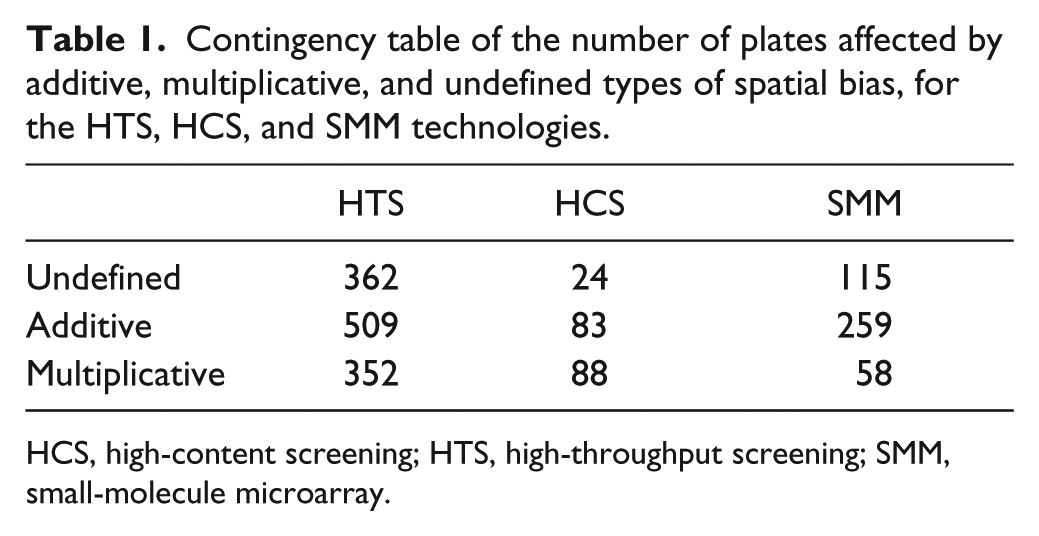
HCS, high-content screening; HTS, high-throughput screening; SMM, small-molecule microarray.

Figure 3 presents the model selection frequencies for our six spatial bias models (Models 1 to 6) among the eight screening categories. Here, the AD test was used to assess the goodness-of-fit of the corrected measurements to the unbiased measurements. According to the AD test, HTS data tend to contain more spatial bias than HCS or SMM data. Moreover, HTS data followed an undefined bias model more frequently than HCS or SMM data (23.7%, 5.8%, and 16.3%, respectively).

Figure 3.

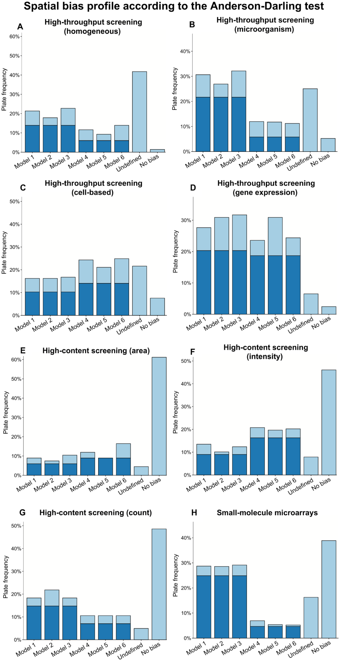
Spatial bias model frequency based on evidence obtained from the Anderson–Darling test for (A–D) high-throughput screening data, (E–G) high-content screening data, and (H) small-molecule microarray data. Control wells were excluded from all computations. Darker portions of bars account for plates without intersections of rows and columns affected by spatial bias; in this case, any additive model (Models 1–3) can be applied when spatial bias was classified as additive, and any multiplicative model (Models 4–6) can be applied when spatial bias was classified as multiplicative. Lighter portions of bars corresponding to Models 1 to 6 account for plates with intersections of rows and columns affected by spatial bias (in this case, the model yielding the largest p-value should be applied).

Figure 4 depicts the bias model selection frequencies according to the CVM test obtained for data of the eight considered screening categories. Similarly to the AD test, evidence from the CVM test indicates that HTS data tend to contain more biased plates that do not correspond to any of the six bias models presented in our study (i.e., the bias model for HTS data was classified as undefined more frequently than for HCS and SMM data). In particular, the bias model was identified as undefined in 44.3% of HTS plates (computed for the four HTS screening categories), compared to 13.5% in HCS (computed for the three HTS screening categories) and 19.5% in SMM.

Figure 4.

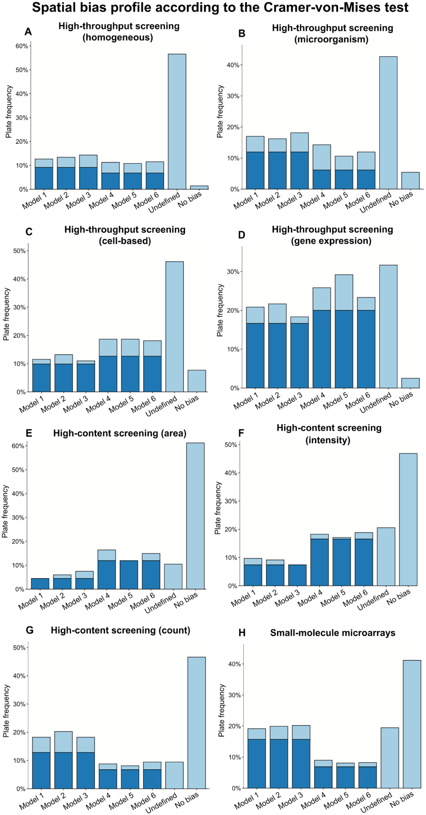
Spatial bias model frequency based on evidence obtained from the Cramer–von Mises test for (A–D) high-throughput screening data, (E–G) high-content screening data, and (H) small-molecule microarray data. Control wells were excluded from all computations. Darker portions of bars account for plates without intersections of rows and columns affected by spatial bias; in this case, any additive model (Models 1–3) can be applied when spatial bias was classified as additive, and any multiplicative model (Models 4–6) can be applied when spatial bias was classified as multiplicative. Lighter portions of bars corresponding to Models 1 to 6 account for plates with intersections of rows and columns affected by spatial bias (in this case, the model yielding the largest p-value should be applied).

Figures 3 and 4 show that only 1.4% of HTS (homogeneous) plates, 5.2% of HTS (microorganism) plates, 7.6% of HTS (cell-based) plates, and 2.4% of HTS (gene expression) plates were unbiased, in contrast to 61.2% of unbiased HCS (area) plates, 46.1% of unbiased HCS (intensity) plates, 48.6% of unbiased HCS (cell count) plates, and 38.9% of unbiased SMM plates. All p-values obtained by applying the McNemar test on 2×2 contingency tables (screening technologies vs. bias model types) were lower than 1×10⁻³. The number of unbiased plates, determined by the Mann–Whitney U test, was the same for both figures.

Let us now examine in more detail the results presented in Figures 3 and 4 . The McNemar test was used to test the differences in proportions mentioned below.

- For HTS homogeneous data ( Figs. 3A and 4A ), spatial bias was found in 98.6% of plates. Here, the CVM test found the same quantity of plates corresponding to an undefined bias model as the AD test (56.6% compared to 41.8%, χ² (1) = 0.16; p = 6.85×10⁻¹). Both the CVM and AD tests found that both multiplicative and additive bias proportions were not different for data of the HTS homogeneous category (χ² (1) = 2.07; p = 1.50×10⁻¹).

- For HTS microorganism data ( Figs. 3B and 4B ), spatial bias was found in 94.6% of plates. The AD test identified much fewer plates with undefined spatial bias than the CVM test (25.0% compared to 42.7%, χ²(1) = 51.51; p = 7.11×10⁻¹³). Both the AD and CVM tests suggest that the additive bias models are more appropriate than the multiplicative ones for data of the HTS microorganism category (χ²(1) = 11.73; p = 6.14×10⁻⁴).

- For HTS cell-based data ( Figs. 3C and 4C ), spatial bias was found in 92.3% of plates. The CVM test suggested that 46.2% of plates have an undefined type of bias, compared to 21.6% of plates according to the AD test (χ²(1) = 15.72; p = 7.34×10⁻⁵). Both tests found that the multiplicative spatial bias model is more adequate for plates of the HTS cell-based category than the additive one (χ²(1) = 0.53; p = 4.65×10⁻¹).

- For HTS gene expression data ( Figs. 3D and 4D ), spatial bias was found in 97.5% of plates. Here, the AD test suggested that 6.5% of plates are affected by an undefined type of bias, compared to 31.7% of plates according to the CVM test (χ²(1) = 37.75; p = 8.03×10⁻¹⁰). The AD and CVM tests did not find a significant difference in proportions of HTS gene expression plates affected by multiplicative or additive types of spatial bias (χ²(1) = 2.50; p = 1.14×10⁻¹).

- For HCS area data ( Figs. 3E and 4E ), spatial bias was found in 38.8% of plates. Both the CVM and AD tests determined that an undefined bias model is rather rare for this type of data (10.4% and 4.5%, respectively, χ²(1) = 44.17; p = 3.01×10⁻¹¹). Here, both statistical tests found no significant difference between the multiplicative and additive spatial bias models (χ²(1) = 0.22; p = 6.38×10⁻¹).

- For HCS intensity data ( Figs. 3F and 4F ), spatial bias was found in 92.1% of plates. The CVM test identified that the bias model was undefined for 20.6% of HCS intensity plates, compared to 7.9% found by the AD test (χ²(1) = 80.65; p = 2.70×10⁻¹⁹). Both the CVM and AD tests did not provide enough evidence that the additive and multiplicative bias models were present in equal proportions in plates generated by the HCS intensity technology (χ² (1)= 0.09; p=7.69×10⁻¹).

- For HCS count data ( Figs. 3G and 4G ), spatial bias was found in 51.4% of plates. Both the AD and CVM tests indicated that only a small proportion of plates follow an undefined spatial bias model (4.9% and 9.5%, respectively; χ²(1) = 96.64; p = 8.30×10⁻²³). No significant difference in proportions of plates affected by additive or multiplicative bias was found here (χ² (1) = 0.74; p = 3.88×10⁻¹).

- For small-molecule microarray data ( Figs. 2H and 3H ), spatial bias was found in 58.8% of plates. Here, the CVM and AD tests determined that 19.5% and 16.3% of plates, respectively, follow an undefined bias model (χ²(1) = 294.35; p = 5.61×10⁻⁶⁶). Both tests also suggested that the small-molecule microarray data tend to be affected by additive bias more frequently than by multiplicative bias (χ² (1) = 9.1; p = 2.56×10⁻³).

In this article, we described the three additive and the three multiplicative spatial bias models along with a general bias detection and removal procedure. We presented evidence that all the six bias models (Models 1 to 6) considered in this study are relevant for the analysis of experimental high-throughput, high-content, and small-molecule microarray data. One of the challenges in spatial bias model selection consists of minimizing the number of plates with an undefined type of spatial bias. The AD test generally outperformed the CVM test in distinguishing between the additive and multiplicative bias models, which resulted in a lower number of plates where spatial bias was classified as undefined. Overall, the AD and CVM tests were in agreement on the spatial bias model that should be used to correct the measurements of a given plate. However, because the AD test is generally more powerful than CVM²² and because it classifies fewer plates as being undefined, it can be recommended for analysis of modern multiwell plates. We also discovered that data generated by HTS technologies are generally more prone to spatial bias than data from HCS and SMM. Although HCS and SMM data are more likely to follow one of the six considered bias models, the bias model in HTS was more frequently classified as undefined, leaving more challenges for future investigations.

The methodology presented in this article is designed to minimize the impact of a plate-specific (additive or multiplicative) spatial bias. A plate-specific bias means that the observed bias patterns appear within a given plate only and may be different for different plates of the assay. An assay-specific bias consists of a bias pattern that appears within all plates of a given assay. A typical example of an assay-specific bias is the case in which a single well location (i.e., measurements taken among all plates of a given assay and corresponding to a fixed well position) gives a very high or a very low reading. An assay-specific bias can be removed by applying the traditional Z-score normalization, first plate-wise and then well location–wise. The traditional Z-score normalization allows one to remove both additive and multiplicative biases when applied to the measurements of a given well location.²⁴ Obviously, the presence of spatial bias in this well location should be primarily confirmed by an appropriate statistical test (e.g., by the Mann–Whitney U test).

The main advantage of our method, compared to the no-correction strategy and the B-score¹⁰ method, is that it copes well with both additive and multiplicative spatial biases by taking into account complex interactions between them. This was confirmed by our simulation study. Obviously, any bias correction method has to be applied with caution. For instance, a screening practitioner should always verify that all tested samples are randomly distributed within given HTS/HCS/SMM plates. If the randomization condition does not hold, some areas of these plates can correctly give very high or very low readings. In this case, the application of bias correction methods may be rather damaging because an unwanted bias may be introduced into the data at hand.

Footnotes

Supplementary material is available online with this article.

Declaration of Conflicting Interests

The authors declared no potential conflicts of interest with respect to the research, authorship, and/or publication of this article.

Funding

The authors disclosed receipt of the following financial support for the research, authorship, and/or publication of this article: This work was funded by the Natural Sciences and Engineering Research Council of Canada (Grant no. 249644) and le Fonds Québécois de la Recherche sur la Nature et les Technologies (Grant no. 173539).

References

Plouffe

D. M.

Wree

A. Y.

, et al. High-Throughput Assay and Discovery of Small Molecules That Interrupt Malaria Transmission. Cell Host Microbe 2016, 19, 114–126.

Lachmann

Giorgi

F. M.

Alvarez

M. J.

, et al. Detection and Removal of Spatial Bias in Multiwell Assays. Bioinformatics 2016, 32, 1959–1965.

Carralot

J. P.

Ogier

Boese

, et al. A Novel Specific Edge Effect Correction Method for RNA Interference Screenings. Bioinformatics 2012, 28, 261–268.

Caraus

Alsuwailem

A. A.

Nadon

, et al. Detecting and Overcoming Systematic Bias in High-Throughput Screening Technologies: A Comprehensive Review of Practical Issues and Methodological Solutions. Brief. Bioinform. 2015, 16, 974–986.

Heyse

Comprehensive Analysis of High-Throughput Screening Data. Proc. SPIE 2002; Bellingham, WA. 2002, 535–547.

Kevorkov

Makarenkov

Statistical Analysis of Systematic Errors in High-Throughput Screening. J. Biomol. Screen. 2005, 10, 557–567.

Makarenkov

Zentilli

Kevorkov

, et al. An Efficient Method for the Detection and Elimination of Systematic Error in High-Throughput Screening. Bioinformatics 2007, 23, 1648–1657.

Malo

Hanley

J. A.

Cerquozzi

, et al. Statistical Practice in High-Throughput Screening Data Analysis. Nat. Biotechnol. 2006, 24, 167–175.

Caraus

Mazoure

Nadon

, et al. Detecting and Removing Multiplicative Spatial Bias in High-Throughput Screening Technologies. Bioinformatics, 2017, 33, 3258–3267

10.

Brideau

Gunter

Pikounis

, et al. Improved Statistical Methods for Hit Selection in High-Throughput Screening. J. Biomol. Screen. 2003, 8, 634–647.

11.

Liu

Sui

Quantitative Assessment of Hit Detection and Confirmation in Single and Duplicate High-Throughput Screenings. J. Biomol. Screen. 2008, 13, 159–167.

12.

Dragiev

Nadon

Makarenkov

Two Effective Methods for Correcting Experimental High-Throughput Screening Data. Bioinformatics 2012, 28, 1775–1782.

13.

Murie

Barette

Lafanechère

, et al. Single Assay-Wide Variance Experimental (SAVE) Design for High-Throughput Screening. Bioinformatics 2013, 29, 3067–3072.

14.

Anderson

T. W.

Darling

D. A.

Asymptotic Theory of Certain “Goodness-of-Fit” Criteria Based on Stochastic Processes. Ann. Math. Stat. 1952, 23, 193–212.

15.

Cramér

On the Composition of Elementary Errors; Almqvist & Wiksells: Stockholm, 1928.

16.

Seiler

K. P.

George

G. A.

Happ

M. P.

, et al. ChemBank: A Small-Molecule Screening and Cheminformatics Resource Database. Nucleic Acids Res. 2008, 36, D351–D359.

17.

Hodges

J. L.

Lehmann

E. L.

The Efficiency of Some Nonparametric Competitors of the t-Test. Ann. Math. Stat. 1956, 324–335.

18.

Tukey

J. W.

Exploratory Data Analysis; Addison-Wesley: Reading, MA, 1977.

19.

Arshad

Rasool

M. T.

Ahmad

M. I.

Anderson Darling and Modified Anderson Darling Tests for Generalized Pareto Distribution. Pakistan J. Appl. Sci. 2003, 3, 85–88.

20.

Kolmogorov

Sulla determinazione empirica di una legge di distribuzione. G. Ist. Ital. Attuari. 1933, 4, 83–91.

21.

Razali

N. M.

Yap

B. W.

Power Comparisons of Shapiro-Wilk, Kolmogorov-Smirnov, Lilliefors and Anderson-Darling Tests. J. Stat. Model. Anal. 2011, 2, 21–33.

22.

Laio

Cramer–von Mises and Anderson-Darling Goodness-of-Fit Tests for Extreme Value Distributions with Unknown Parameters, Water Resour. Res. 2004, 40, W09308.

23.

Stephens

M. A.

Tests Based on EDF Statistics, in Goodness-of-Fit Techniques. JASA 1986, 69, 97–194.

24.

Mazoure

Nadon

Makarenkov

Identification and Correction of Spatial Bias Are Essential for Obtaining Quality Data in High-Throughput Screening Technologies. Sci. Rep. 2017, 7, 11921.

Supplementary Material

Please find the following supplemental material available below.

For Open Access articles published under a Creative Commons License, all supplemental material carries the same license as the article it is associated with.

For non-Open Access articles published, all supplemental material carries a non-exclusive license, and permission requests for re-use of supplemental material or any part of supplemental material shall be sent directly to the copyright owner as specified in the copyright notice associated with the article.

0.00 MB

0.03 MB

Identification and Correction of Additive and Multiplicative Spatial Biases in Experimental High-Throughput Screening

Abstract

Keywords

Introduction

Methods

Spatial Bias Detection in Multiwell Plates

Correction of Plate-Specific Bias

Model 1: Additive Model

Model 2: Additive Model with Arithmetic Mean at the Intersection

Model 3: Additive Model with Multiplicative Interaction of Biases at the Intersection

Model 4: Multiplicative Model

Model 5: Multiplicative Model with Arithmetic Mean at the Intersection

Model 6: Multiplicative Model with Geometric Mean at the Intersection

Model Selection for Removing Plate-Specific Spatial Bias

Traditional and Modified Partial Mean Polish Algorithms

Choice of Statistical Test to Determine the Bias Model

Simulations

Results and Discussion

Footnotes

Declaration of Conflicting Interests

Funding

References

Supplementary Material