
Abstract
OpenStreetMap (OSM) is now an important data source for many mobility services. In particular, the OSM road network model is often used by cycling applications and studies. A very common operation with cycling data is map-matching, where the GPS traces of cycling trips are matched against the road network model. However, cyclists can take many unconventional paths that do not always match the official road network model. This fuzziness can severely compromise the ability of map-matching algorithms to produce valuable results. In this work, we introduce the concept of map-matching anomaly as a systematic mismatch between cycling traces and the road network data model to which the traces are expected to be matched. Contrary to sporadic map-matching errors, anomalies will recurrently occur for similar traces and will therefore accumulate at specific locations. This paper proposes a methodology to support the systematic and large-scale identification of map-matching anomalies in urban environments and discusses how knowledge about these anomalies can help cities uncover novel and actionable insights about cycling behaviour. The proposed methodology achieved 84% precision in identifying locations prone to map-matching anomalies. We identified several cases where the OSM road network was incorrect or incomplete. We also identified several locations where a deeper intervention is needed to improve the road network infrastructure.
Introduction
As part of the growing interest in using digital tools to support cycling activities, OpenStreetMap (OSM) has gained significant relevance as an enabling technology for various cycling applications and services. OSM is a free and open repository of geographic information (Barrington-Leigh and Millard-Ball, 2017) providing information for various types of applications, such as route planning (Nunes et al., 2021), cycle parking planning (Ito et al., 2023), behaviour assessments (Sultan et al., 2017), and bikeability analysis (Beecham et al., 2023). OSM is curated by a large community, which includes individual mappers, informal OSM communities, for-profit organisations, and paid editors (Anderson et al., 2019). They are responsible for keeping OpenStreetMap (OSM) up-to-date, for example, by mapping information about the road network, buildings, or administrative limits. They rely on three basic elements to represent geographical features, namely, nodes, ways, and relations, and can assign one or more tags to describe the properties of a feature (OpenStreetMap contributors, 2025a, 2025b).
The ability to accurately represent real cycling traces is a core requirement for OSM to become an enabling technology for cycling information systems. OSM data represents the existing road network, including information on the bikeability of the roads. Mappers can use the ‘highway=cycleway’ tag to express separate cycleways, and, in cases where the cycling infrastructure is part of a road, mappers can add the ‘cycleway=*’ tag to an existing way (‘highway=*’) (OpenStreetMap contributors, 2025c, 2025d). This information is the building block for navigation services that suggest the most suitable cycling routes and for mobility analysis tools that help decision-makers plan cycling infrastructures.
In addition to route representation, it is also essential to collect and represent data about actual cycling activity. This information is usually collected as GPS traces, sequences of GPS coordinates representing paths travelled by cyclists. Many local authorities are now collecting this data to obtain an overview of the mobility patterns of cyclists in their cities. There are already various ways of processing this type of data, many of which have been extensively studied (Chung et al., 2024; Poliziani et al., 2022; Schweizer et al., 2020). A common technique to create an aggregate perspective of multiple GPS traces is to align them to a road network model, a process called map-matching (Brakatsoulas et al., 2005). By map-matching many cycling traces, one can remove the errors and variations embedded in each GPS trace and associate them all with a common road network data model, upon which it becomes possible to perform further mobility analysis, such as to uncover route choice preferences (Chung et al., 2024) or the waiting times at intersections (Poliziani et al., 2022).
The efficacy of map-matching processes highly depends on the ability of the road network data model to provide a comprehensive representation of vehicle routes. However, while most maps generally provide excellent support for motor vehicle routes, they often have insufficient support for cycling (Chen et al., 2023). At the core of the problem seems to be the assumption that cyclists will either follow cycle infrastructure or share the roads with cars. Therefore, cycling traces are assumed to correspond to routes matching one of these two possibilities. In reality, cycling paths are much fuzzier. A realistic cycling journey may involve frequent switching between heterogeneous roads with different profiles and purposes, such as footpaths, parks, and other unconventional paths that are often not represented on a road network model or at least not as being cyclable (Schweizer et al., 2016). Mekuria et al. (2012) describe two opposing definitions for a bike network: Municipalities define it as a set of links where cycling is officially permitted, while cyclists define it as a set of roads and paths not exceeding their tolerance for traffic stress.
This ambiguity about the concept of bike network can seriously compromise the ability of the road network data model to completely represent the paths that cyclists effectively follow, making map-matching more likely to fail. In some cases, the process results in map-matching errors where the algorithm fails to produce any match between a GPS trace and the road network data model. In other cases, the map-matching does not produce any error, but it returns a map-matched route that differs from the source GPS trace. In other words, the map-matching output is valid, in the sense that it is based on the road network data model, but it is not representative of the cyclist’s actual trace. This issue cannot be addressed only from the perspective of map-matching errors. If the road network data model does not offer any reasonably suitable route to represent a particular GPS trace, then there is not much that map-matching can do to produce a viable match.
However, these erroneous interpretations of cycling activity lead to incorrect inferences about route preferences (Berjisian and Bigazzi, 2023) and significantly affect the value that can be offered by cycling information services (Velaga et al., 2012), for example, route suggestions may fail to consider popular but misrepresented cyclists’ paths. Despite recent advances in detecting and understanding the limitations of map-matching techniques (Berjisian and Bigazzi, 2023; Carvalho et al., 2024; Dey et al., 2022), there is still limited research on this topic (Qu et al., 2023). Identifying these anomalous cases still involves visual inspection and reasoning (Dey et al., 2022), usually in the context of a single GPS trace.
In this study, we aim to go beyond the challenges of map-matching and focus on the challenges emerging directly from the discrepancies between cycling traces and their representation in OSM. To clearly distinguish this problem from the common limitations of map-matching algorithms, we start by defining the concept of map-matching gap and introducing the novel concept of map-matching anomaly in Definitions 1 and 2, respectively.
Map-matching gaps correspond to any situation in which the attempt to map-match a cyclist’s GPS trace into the OSM road network results in a map-matched route that does not accurately represent the original trace.
A map-matching anomaly is a systematic discrepancy between the road network data model and a pattern of GPS traces crossing a specific area. Such a discrepancy induces map-matching to systematically produce map-matching gaps when attempting to map-match GPS traces crossing a specific area.
Therefore, anomalies are not a consequence of GPS errors or of any limitations in map-matching algorithms. Not even the best possible map-matching algorithm applied to a perfect GPS trace would be able to produce a suitable representation of the source GPS trace because no such route exists in the road data network model. The result will inevitably be an anomalous representation of that source GPS trace.
The recognition of map-matching anomalies and a deeper understanding of their impact can strongly affect the narrative associated with the map-matching of cycling GPS traces. When considering a single cycling GPS trace, map-matching gaps are not as relevant because there are several other sources of problems, such as GPS errors. In addition, a single map-matching gap might just be an occasional event in which a single cyclist followed some unconventional path. However, when considering the systematic map-matching of large numbers of cycling traces in the context of a city, anomalies become much more relevant than the errors within any individual GPS trace. While GPS errors produce some noise, they end up being distributed and often compensate for each other in the global view provided by many GPS traces. On the contrary, anomalies are associated with specific places and represent systematic errors because they result directly from the limitations of the local road network model in that area. This is why anomaly detection will only be meaningful for large concentrations of GPS traces that may support the systematic identification of those anomalies.
Therefore, anomalies can have a significant impact on the interpretation of cycling activity represented by a large number of cycling traces in the same region. They generate a systematic distortion of reality that will inevitably lead to wrong assumptions and decisions about cycling activity.
Objectives
We aim to study the challenges emerging from the existence of gaps between real cycling traces and their representation in OSM. We defined the following two objectives: • •
Analysing map-matching anomalies can help municipalities and OSM collaborators detect areas where the reality of cycling traces systematically diverges from the matching of those traces into the road network data model. Knowledge about these anomalies may help them identify opportunities for improvement. These improvements may include changes in OSM representation of cycling routes, suggestions for infrastructural changes, or even tips for cyclists. This contribution may help improve future cycling applications, generate better route suggestions, and produce novel insights about cycling behaviour. It is important to note that the method proposed in this study should be independent of the specifics of the map-matching algorithm used.
Paper structure
The article is structured as follows: The next section reviews the current state of the art. Section “Methodology” describes the overall methodology for identifying map-matching anomalies, and section “Step description and results” details each step and presents the results of applying this methodology to a real dataset. The subsquent section discusses how overcoming anomalies can enhance cycling conditions. Finally, the “Conclusions” Section summarises the main findings and outlines potential directions for future research.
Related work
Previous literature has addressed this issue from two major perspectives: The first perspective focuses on the limitations and quality of OSM, while the second focuses on the map-matching processes and their limitations.
OSM road network completeness
The popularity and widespread use of OSM have led many authors to assess the quality and completeness of OSM data. Overall, studies have shown that OSM data has relatively good quality and particularly high quality for designated lanes (Hochmair et al., 2015). In some cases, it is even more complete than official datasets (Ferster et al., 2020), as informal paths and new infrastructures are often mapped in OSM before they are released on official datasets (Nelson et al., 2021). Comparing OSM to reference datasets, roads tagged as ‘on-street bicycle lanes’ appear the most concordant, while cycle tracks and local street cycleways appear the least concordant (Ferster et al., 2020).
Globally, OSM is found to be 83% complete, and in 40% of the countries, it covers more than 95% of the roads (Barrington-Leigh and Millard-Ball, 2017). OSM is found to be a reliable tool for many applications, for example, for computing the Level of Traffic Stress metric (Wasserman et al., 2019) and for vehicle routing applications (Graser et al., 2015). However, Viero et al. stated that OSM has insufficient quality for performing network-based analysis of cycling conditions (Vierø et al., 2024).
Despite its good quality, Hochmair et al. (2015) identified two common types of errors, namely, omission and commission. Omission errors occur when a cycle lane is not represented in the OSM or misses proper tags, while commission errors occur when OSM includes non-existent roads or roads with incorrect geometries or tags. Due to its crowdsourced nature, a key challenge is to achieve consistent OSM tagging. Not all mappers have sufficient training in geography and surveying, and those who do might often employ diverse labelling practices, leading to inaccurate, incomplete, inconsistent, or vague contributions (Basiri et al., 2016; Ferster et al., 2020; Nelson et al., 2021). Some street typologies and urban contexts are more prone to errors. Completeness has a U-shaped relationship with population density; both sparsely populated areas and dense cities seem to be the best mapped (Barrington-Leigh and Millard-Ball, 2017).
Map-matching
Map-matching is a key process in modelling mobility. Given a road network model and a GPS trajectory of a vehicle, it tries to find the most probable sequence of road network edges on which the vehicle has travelled (Yang and Gidófalvi, 2018). However, applying map-matching for cyclists traces is particularly challenging, as cyclists frequently use paths that are not designed for cycling or that might not be included in the road network data, such as parks or shortcuts (Berjisian and Bigazzi, 2023; Schweizer et al., 2016). The built environment also influences the performance of map-matching algorithms. In areas with a complex road network, the probability of having map-matching anomalies is higher than in zones with a sparser road network (Trogh et al., 2022).
Several authors have targeted these challenges and proposed new map-matching algorithms specifically designed for cycling mobility. Schweizer et al. (2016) proposed a method that uses network attributes to estimate the route in case of incomplete GPS data and can identify if cyclists used a reserved bikeway. There also methods that favour bikeways extracted from OSM (Bergman and Oksanen, 2016), while others discard some roads depending on the transportation mode (Trogh et al., 2022). The method proposed by Gao et al. (2024) classifies road availability for cyclists to help during the map-matching process.
Some authors acknowledge the incompleteness of road network data and propose approaches capable of performing off-road map-matching or detecting road network errors. Murphy et al. (2019) proposed a method that generates and uses off-road trajectories as a fallback when the road network cannot accommodate the vehicle trajectory. Behr et al. (2021) proposed a method that extends the road network data model by triangulating all open areas and adding tessellation edges and considers each GPS point as a possible matching candidate, adding them to the road network graph if no match is found. Yang et al. (2024) used a neural network model to detect various categories of road network errors using extracted context features from the map-matching outputs, raw trajectories, and road network.
The off-road sections can then be used to interpolate missing road segments and to update the road network (Sasaki et al., 2019; Shan et al., 2015). The authors assume that, since vehicles are usually restricted to the road network, unmatched trajectories can be used to find new roads (Tang et al., 2019). Although this approach is reliable for cars, cyclists’ paths may correspond to illegal roads or connections and thus may not be eligible to be represented in a road network. OSM collaborators often follow the on-the-ground mapping rule, which states that the world should be mapped as it is physically observed (OSM, 2025).
In a different approach, some authors have studied the identification and characterisation of map-matching errors. Berjisian and Bigazzi (2023) used several similarity measures to compare the GPS trace with the map-matching output and flag cases requiring visual inspection. Dey et al. (2022) proposed a two-phase methodology that uses an unsupervised learning model to help classify map-matched segments as good or bad based on the quality of GPS points and uses the ‘edit distance’ metric to detect unrealistic travel behaviour. Carvalho et al. (2024) combined supervised machine learning with similarity measures to detect and classify gaps between GPS traces and map-matched routes.
In this work, we explore this problem in further detail and extract the exact portions of a GPS trace leading to map-matching gaps. Compared to our previous work, as described in (Carvalho et al., 2024), we shifted from a broad identification of gaps to a more specific identification of where exactly the gaps happen within the GPS trace. By applying this process to a large dataset, we remove the influence of sporadic events and identify which zones in a city are prone to anomalies. We do not assume that all gaps occur only due to road network or GPS errors but also due to cyclists’ habits or even internal map-matching errors.
Methodology
According to our definition, a map-matching anomaly occurs when the map-matching algorithm systematically produces errors or generates alternative routes that misrepresent a pattern of GPS traces crossing a specific area. Figure 1 provides three map-matching gaps to illustrate three scenarios corresponding to our anomaly definition. The figure also shows how a single GPS trace (red dotted line) can result in multiple map-matching segments (blue arrow lines). The thinner grey lines represent the base road network, and the dashed circles highlight the three map-matching gaps. While we only represented one gap per anomaly to simplify interpretation, in reality, there would be a large concentration of gaps around each anomaly, forming a cluster. A GPS trace, its map-matched polylines, and three map-matching anomalies.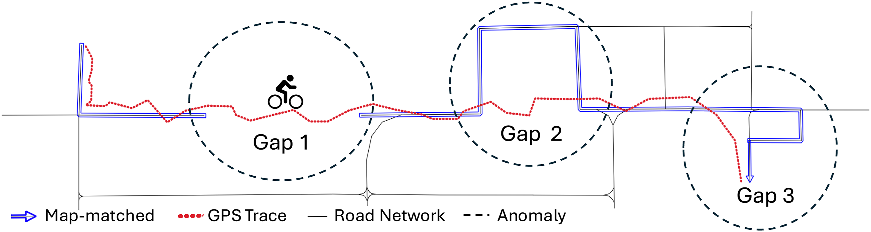
In Figure 1, map-matching Gap 1 represents cases in which map-matching fails to produce any match and returns an error. Gap 2 represents cases where no viable match exists, but the algorithm generates a detour, a route that is not representative of the trace. Finally, Gap 3 represents the cases where, despite a better candidate road, the algorithm did not consider it eligible for map-matching the cycling traces. This includes scenarios where cyclists ride against traffic on one-way roads or travel on walkways. In all these cases, an anomaly exists because in the road network model, there are no viable roads to represent the cyclist’s path. This lack of representation will inevitably lead the map-matching process to produce systematic map-matching gaps.
The methodology proposed in this paper to identify map-matching anomalies is based on a large dataset of cycling trips collected in Braga, Portugal. These data were collected as part of a collaboration between Braga Municipality and the Bicification project.
1
In this project, cyclists could receive monetary rewards for logging their bike trips in the city using a mobile application. This was a cycling incentive and a way to collect valuable and reliable trajectory data. Within the period of analysis, between 31/05/2022 and 26/09/2022, 262 cyclists produced 16,292 GPS traces, corresponding to 94,467 km of cycling trajectories. Figure 2 shows a heatmap with the spatial distribution of the GPS traces across Braga, where each red line represents a single GPS trace. Braga is a mid-sized city with approximately 150,000 inhabitants. This large concentration of cycling trips in a relatively small region was very valuable for the goals of our study, providing us with enough data points to assess cycling patterns and move beyond the circumstantial analysis of particular trips. The heatmap with the spatial distribution of the GPS traces in the Bicification dataset.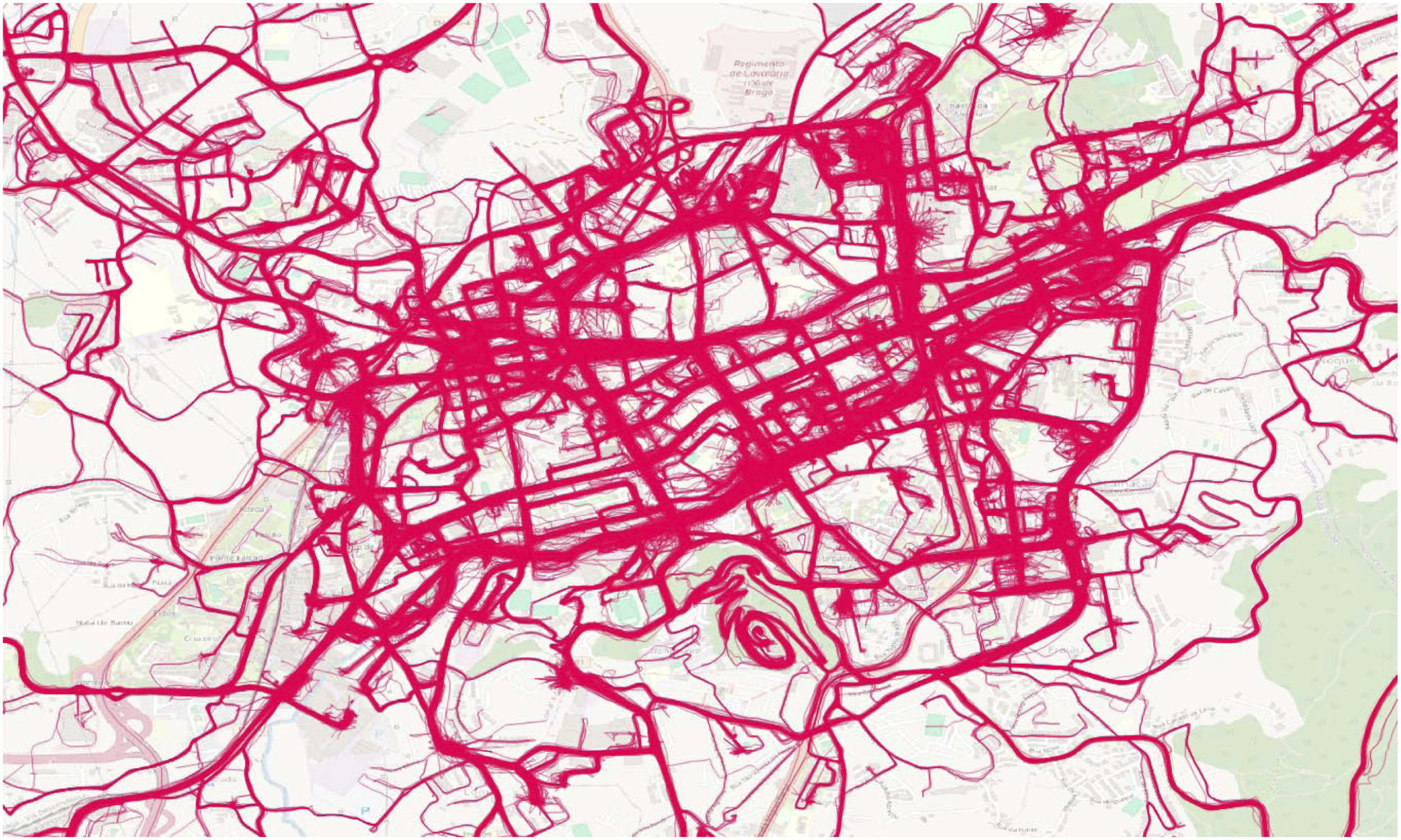
Figure 3 describes the proposed methodology for identifying areas prone to map-matching anomalies. This process consists of four steps, namely, map-matching, anomaly extraction, anomaly clustering, and anomaly analysis. A four-step methodology for anomaly identification and analysis.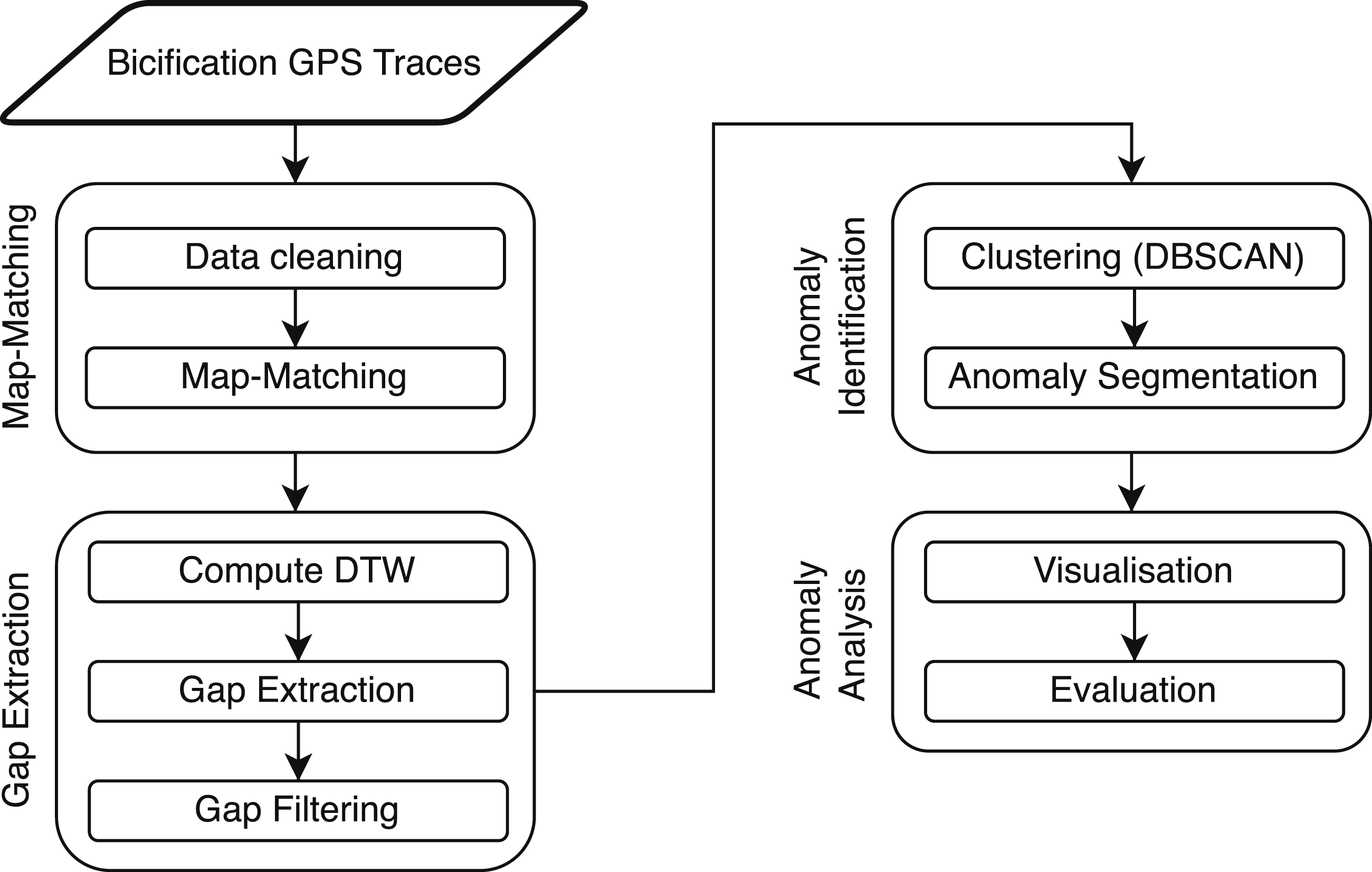
We started by cleaning the Bicification dataset and map-matching the eligible GPS traces to the OSM road network. Then, we analysed the map-matching results to identify the anomalies. This included comparing each GPS trace with its map-matched polylines using reference similarity measures to identify and extract the portions where both geometries appear less similar. Finally, we applied a spatial clustering algorithm to identify the areas of the city where these anomalies occurred systematically.
The next section presents a detailed description of each step, and, right after each description, it presents the results of applying each step. This approach provides essential context for understanding the subsequent steps. This structure facilitates comprehension of the logical flow of the proposed method.
Step description and results
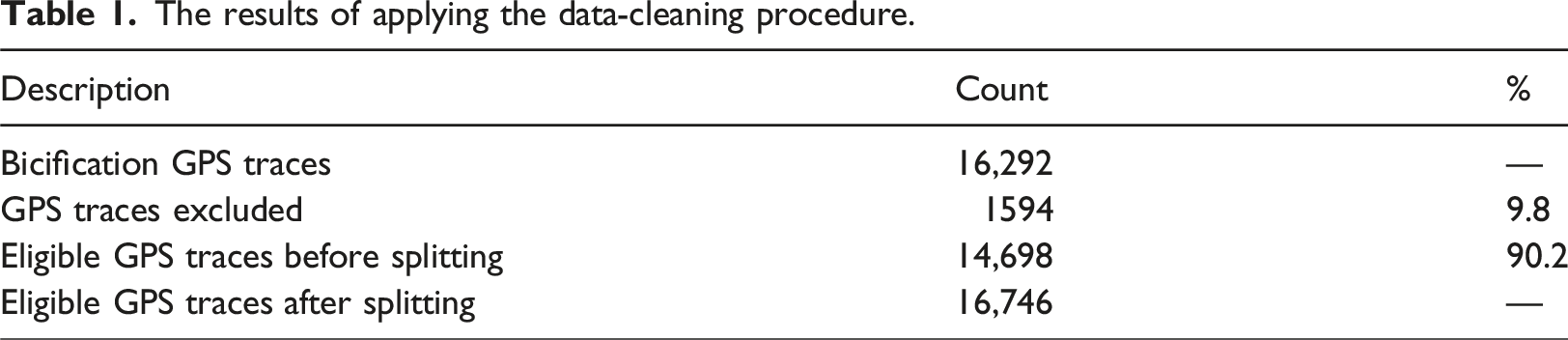
We started by conducting a data-cleaning procedure to remove abnormal situations from the original dataset. We first excluded the GPS traces recorded outside our area of interest, specifically within the boundaries of Braga City. Then, to reduce the impact of low-quality GPS traces, we split any GPS trace where two consecutive points were at least 200 m apart into separate traces. Such gaps in a trajectory often occur due to GPS signal loss or temporary interruptions in data recording. Removing these gaps helps prevent false positives.
The results of applying the data-cleaning procedure.
Map-matching
In the map-matching step, we applied a map-matching algorithm to align the eligible GPS traces to the OSM road network. For this purpose, we used the map-matching service developed by Mapbox, which is a reference solution in this domain and supports OSM road network data models. We configured the map-matching service to consider the bicycle profile, which is described to avoid highways and give preference to streets with bike lanes. It is worth stressing that our work is not about the quality of map-matching algorithms. We are specifically looking for map-matching anomalies. While our results could be slightly different using other map-matching tools or by different map-matching parameterisation, our map-matching anomaly concept is inherent to the road network data models and therefore should be largely independent from the specifics of any map-matching algorithm. In the case of map-matching parameterisation, such flexibility is expected. Regions may have different rules for similar scenarios. For example, in some regions, cyclists may be allowed to ride against traffic, whereas in others such behaviour is prohibited. Thus, what may constitute an anomaly may vary across regions, and the anomaly identification process should be adaptable to these perspectives.
The Mapbox map-matching API
2
accepts a sequence of 2 to 100 GPS coordinates as input, and the response of a map-matching request will fall into one of the following 3 categories: (i) Map-matching error: The GPS trace could not be map-matched into the OSM road network. The result is an execution error, and no route is returned. (ii) One map-matched polyline: The GPS trace was map-matched into a single polyline, a sequence of route segments. (iii) Multiple map-matched polylines: The GPS trace was map-matched into several polylines. This indicates that some portions of the GPS trace could not be map-matched into the OSM road network, resulting in discontinuities.
To ensure optimal results in the map-matching process, we preprocessed the 16,746 eligible GPS traces to ensure that consecutive GPS coordinates were at least 10 m apart. Additionally, due to the GPS coordinate limit per request, eligible GPS traces exceeding this limit were divided into segments of 100 points each, with the last segment potentially containing fewer points.
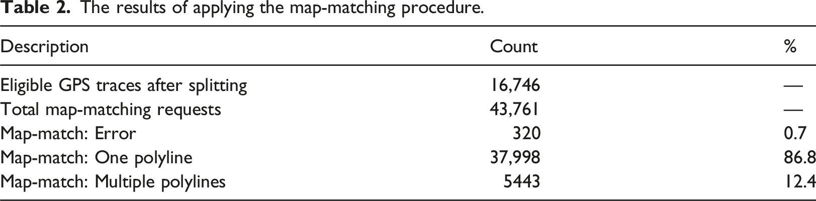
The results of applying the map-matching procedure.
Gap extraction
The gap extraction step aims to identify and extract the map-matching gaps. Cases where map-matching failed to produce any match were straightforwardly considered as a map-matching gap. The main challenge is to define rigorous criteria to identify gaps corresponding to routes that misrepresent the source trace. To address this challenge, in the cases where the map-matching produced one or multiple map-matched polylines, we used the Dynamic Time Warping (DTW) algorithm (Müller 2007) and the Optimal Warping Path (OWP) to compare the GPS trace with its corresponding map-matching polyline and identify the segments of both geometries that are below a certain level of similarity. DTW is a technique to find the optimal alignment between two sequences (time series) (Müller, 2007) and is widely used in different fields, such as speech recognition, trajectory similarity (Tao et al., 2021), and dynamic signature verification (Jiang et al., 2022). For two sequences, the DTW value is well-defined; however, they can have different warping paths. The OWP is a path that optimises the sum of all local distances. A local distance refers to the distance between two elements of each sequence based on a cost function. The cost function can be defined according to the purpose of the study. In our study, the sequences are composed of WGS84 coordinates. Therefore, we used the Haversine distance formula as the cost function.
It is important to note that before computing the DTW, we interpolated points every 2 m in the GPS and map-matched geometries. This solution reduced the impact of long intervals between consecutive points, which would lead to high local distances during the OWP computation, even when both geometries appear similar.
After computing the OWP, we classified map-matching gaps as corresponding to cases where the local distance was higher than 10 m for at least five consecutive points. Where a map-matching gap was detected, we registered the gap segment and its gap trace. The former corresponds to segments in the map-matching response, and the latter corresponds to the part of the source GPS trace that produced the gap.
Results: In total, we extracted 153,170 map-matching gaps. Figure 4 presents 2 examples of those gaps. The red dotted line represents the gap trace, while the blue represents the gap segment. Example of two different map-matching gaps detected.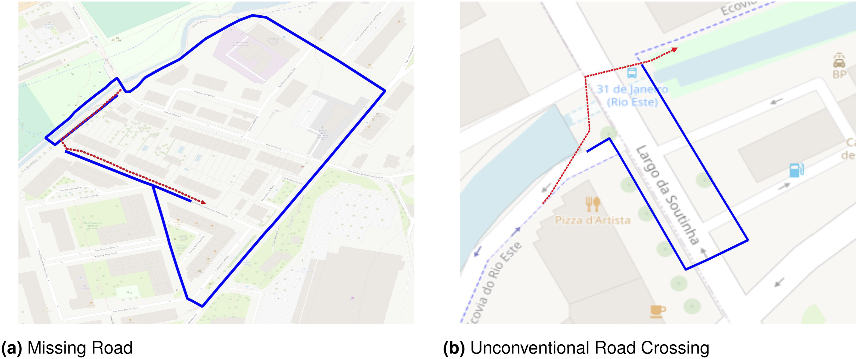
Figure 4(a) illustrates a scenario where the cyclist used a ramp not mapped in OSM to transition from a cycleway to a residential road. The map-matching algorithm attempted to find a path connecting the cycleway and the residential road. Figure 4(b) shows a situation where the cyclist crossed the road outside the designated area. The map-matching algorithm snapped the GPS trace to the nearest zebra crossing.
Gap filtering
A large number of the map-matching gaps produced in the previous step correspond to very short route segments. To focus on an aggregate perspective and avoid many false positives, we decided to remove gaps where the gap traces were shorter than 40 m or where the ratio between the length of the gap trace and the gap segment was between 0.7 and 1.3. We consider false positives the case in which the map-matching algorithm successfully snapped the GPS into the correct road, but GPS interferences created a deviation in the GPS trace sufficient to induce our algorithm to consider it as a gap.
We also removed gaps where the gap trace consisted of the beginning or end sections of the GPS trace. These sections can easily lead to map-matching errors due to the calibration of the GPS sensor or the map-matching algorithm itself. While GPS problems could be addressed in the data-cleaning step, the interferences from map-matching calibration can only be detected in this phase.
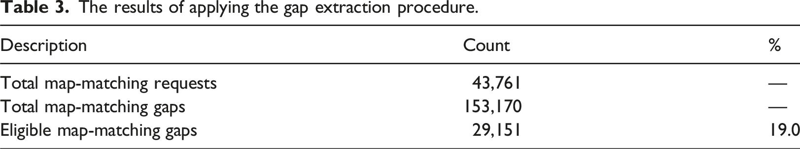
The results of applying the gap extraction procedure.
During our analysis, we observed that most gaps with a ratio greater than 1.3 were removed, as they involved the beginning or end sections of the GPS traces.
Anomaly identification
In the anomaly identification step, we aimed to identify locations where gaps concentrate. The goal is to create an aggregate view of these gaps, focussing on their quantitative relevance, especially on truly systematic cases, indicating an underlying problem. A large cluster may not only be large due to having many gaps but also because it aggregates several smaller clusters that, despite having different characteristics such as movement patterns, share the same underlying cause. For this purpose, we applied the DBSCAN 3 clustering algorithm. To apply this procedure, we selected the midpoint in each gap trace since the midpoints of gaps passing through the same area tend to converge to the same location.
The rationale behind this procedure is that in zones where the road network does not represent the cyclists’ paths, map-matching is likely to produce recurring gaps, leading to areas with a high concentration of gaps. In contrast, sporadic events, such as strong GPS interferences or map-matching malfunctions, mainly result in spatially dispersed gaps. As DBSCAN groups data points based on spatial proximity, it mitigates the impact of sporadic events and highlights the most common gaps.
DBSCAN requires two parameters: the minimal number of points composing a cluster and the distance threshold (epsilon). After some experimental iterations, we selected a fixed epsilon of 15 m and a minimum number of 20 points. However, the optimal value for these parameters may vary depending on the number of gaps extracted, especially the minimum number of points. As the number of gaps increases, the minimum point threshold should be adjusted accordingly to prevent the formation of overly large and dispersed clusters.
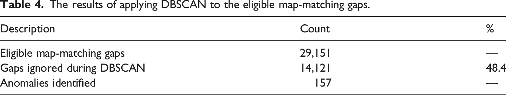
The results of applying DBSCAN to the eligible map-matching gaps.
Analysing the distribution of the number of gaps per anomaly, we could verify that of the 157 anomalies obtained, 125 anomalies had fewer than 100 gaps. On the opposite side, nine anomalies contained more than 420 gaps. In particular, the two most significant anomalies contained more than 1000 gaps. Although anomalies are recorded in various areas of the city, this relative distribution shows that certain areas require greater prioritisation. Targeted interventions in these high-density clusters can benefit a substantially larger number of users.
Anomaly segmentation
DBSCAN clusters were formed solely based on the geographical location of the midpoints of gap traces. Consequently, an anomaly may include gap traces with similar locations but differing movement patterns (e.g. direction, origin, destination, and distance). In some cases, these differing patterns jeopardise the interpretation process. To simplify anomaly analysis, we could visualise each gap trace individually. However, searching for similar or different patterns within an anomaly containing thousands of gaps with varied movement patterns is time-consuming.
To calculate these trace patterns, we implemented an additional step using the DTW measure to subdivide the gap traces of a cluster into smaller groups matching the same movement pattern. This step is described in Algorithm 1. This algorithm takes as input a set of gap traces that constitute an anomaly and groups them into one or more patterns. It has three parameters: the minimum number of gap traces that have a match (M), the maximum DTW value to consider two gap traces ‘similar’ (T), and the number of ‘similar’ gap traces to consider when computing DTW (N).
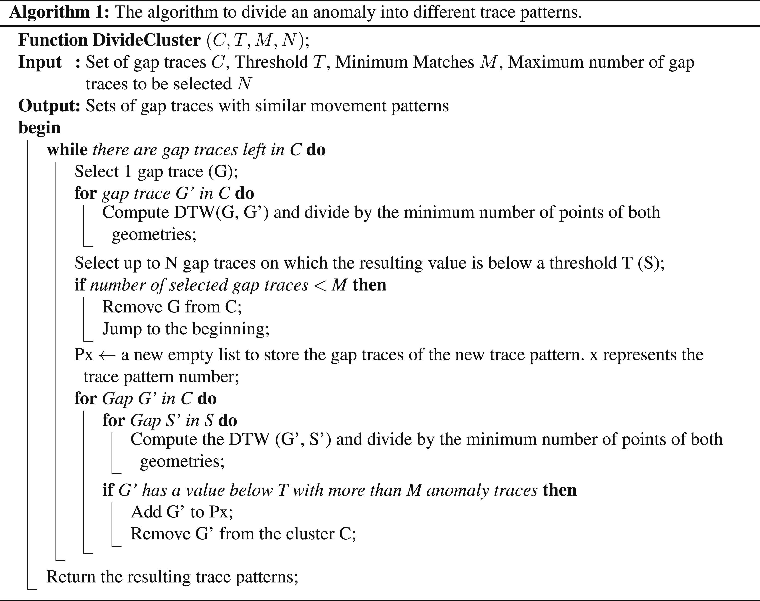
In this study, we tested different values and combinations for each parameter, namely, M: [3, 5], T: [15, 25, 30], and N: [10, 12]. It is important to note that our aim was not to optimise and evaluate the performance of this algorithm, but to facilitate the cluster analysis.
Results: Figure 5 shows the number of trace patterns obtained per anomaly. The image shows that the majority of the anomalies (64%) have 1 or 2 trace patterns. Cluster segmentation results: The number of trace patterns per cluster.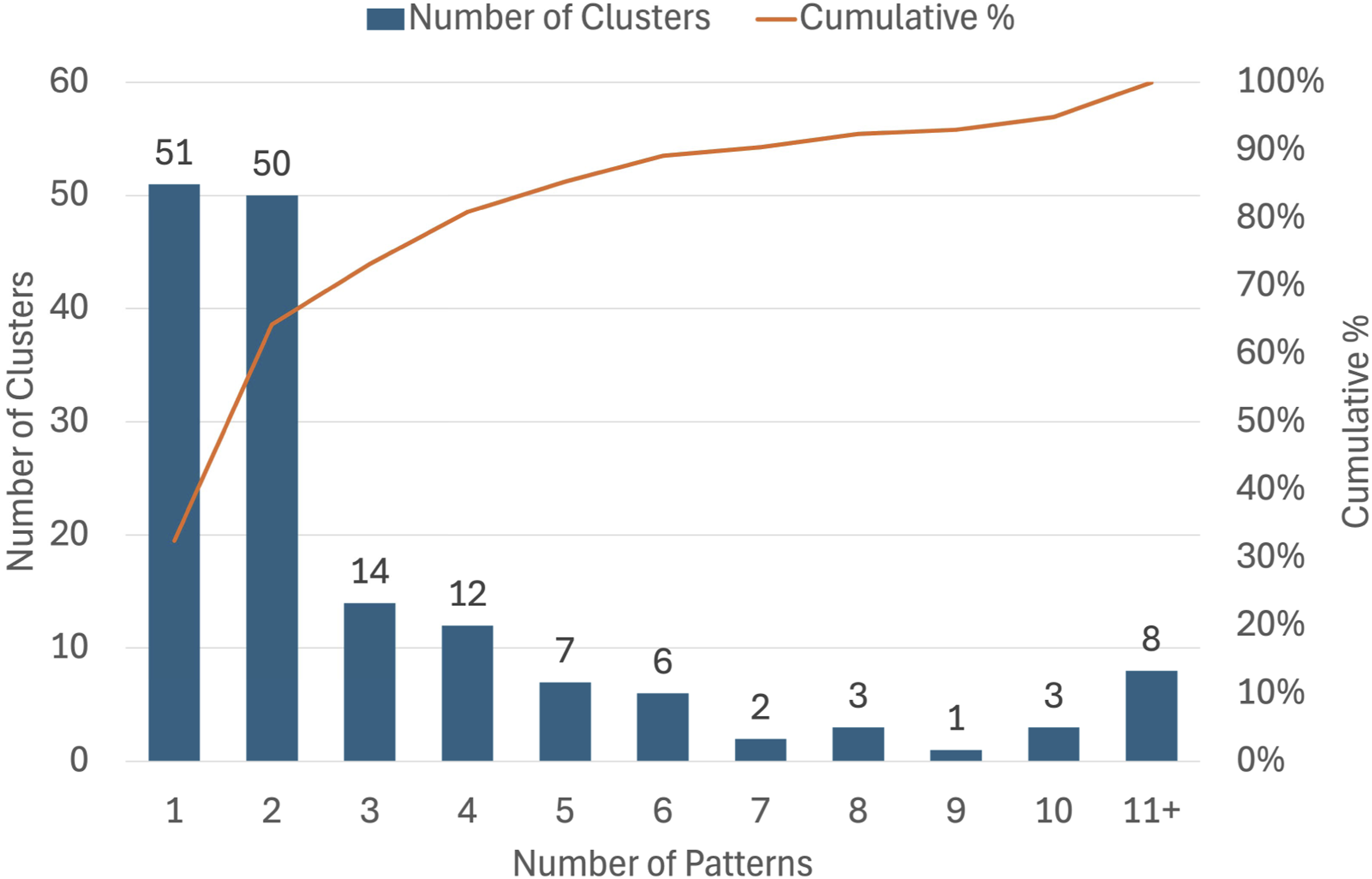
By visually inspecting the results, we could observe that frequently the two trace patterns with the most gaps represent the same path but in opposite directions, such as the two trace patterns depicted in Figure 6(c1) and (c2). The remaining trace patterns may represent small variations in the path, such as a different origin as depicted in Figure 6(c3), or a completely different path, such as in Figure 6(c4). Different levels of analysis: (a) Global, (b) anomaly, (c) pattern, and (d) gap.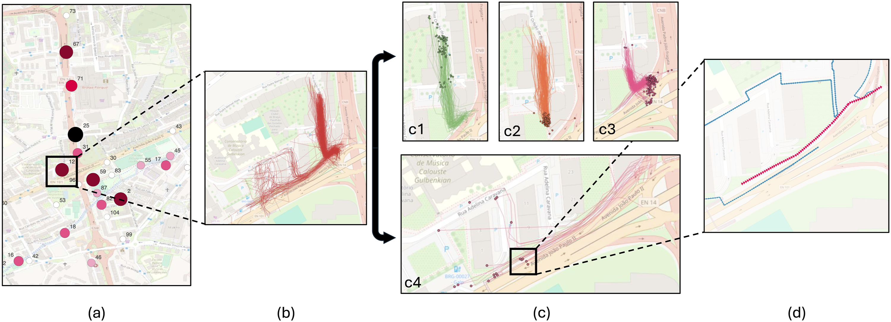
Anomaly analysis
Evaluation of the anomalies.
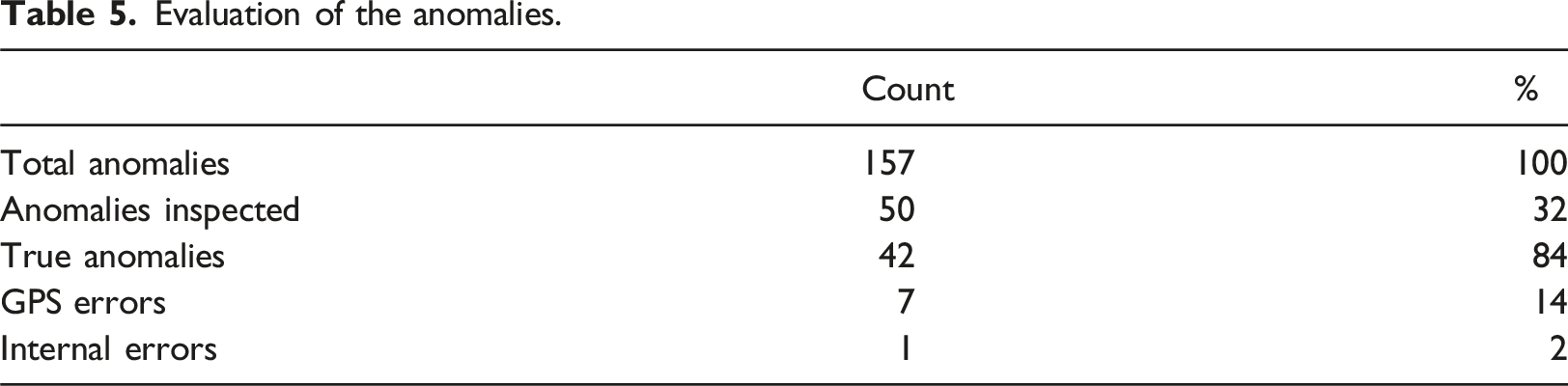
In total, we identified 42 true anomalies, cases where the map-matching algorithm failed to produce the correct representation of cyclists’ traces due to limitations in the road network model. This corresponds to a 84% precision rate. This was especially common when cyclists used sidewalks to avoid travelling along or against traffic, changed roads at unconventional locations, or rode through parks and open spaces.
Another significant source of anomalies was the behaviour of the Mapbox map-matching algorithm, which, when configured for a cycling profile, excludes roads tagged as ‘trunk;’ from the set of eligible paths for cycling. In such cases, the algorithm either failed to return any match or inaccurately snapped the route to the nearest eligible road segment.
We identified 7 cases where map-matching failed due to strong GPS interferences. Some of them were caused by situations where the cyclist remained stationary at a location. The data-cleaning process did not account for these cases, but they could be mitigated by applying specific pre-processing techniques.
We also identified one case where the anomaly was due to the map-matching algorithm. Specifically, this case was caused by two parallel roads. When there are two or more parallel roads nearby, even small interferences in the GPS signal can induce the map-matching algorithm into errors. These types of errors are difficult to identify just by comparing the geometry of both polylines. Even when visually inspecting the results, without the ground truth about the cyclists’ paths, we cannot assert whether they shared the road with motorised traffic or used the sidewalk.
Discussion: Overcoming anomalies to improve cycling
In the first part of the paper, we addressed the objective of developing an unsupervised method to extract map-matching gaps and identify anomalies. In this section, we revisit the second objective by analysing how anomalies can help cities uncover novel insights into cycling behaviour.
We begin by breaking this research objective into two perspectives: The macro or global analysis, a city-scale exploration of cycling behaviour, and the micro or local analysis, a detailed investigation of specific locations or individual cyclists.
Macro analysis
In a macro analysis, the stakeholders may wish to obtain an overview of the severity of anomalies, monitor how the volume and characteristics of anomalies vary during the day, across city areas or in different cities, and benchmark the overall alignment between cycling activity and the road network model. They may wish to examine how anomalies relate to road accidents, road types, motorised traffic intensity, district characteristics (e.g. residential or commercial) or critical locations (e.g. schools or hospitals). This broad perspective enables cities to identify priority areas and benchmark the design of their cycling infrastructure.
To conduct macro-level analysis, it is ideal to establish a set of metrics that can be computed automatically on a large scale. This approach ensures that the methodology is replicable across different cities, allowing effective benchmarking and comparison. Some of these metrics may be computed at the city level or at a finer spatial scale. The latter describes a neighbourhood or district in finer detail. Additionally, it should be possible to aggregate them into a global metric to represent the overall conditions of the city. Examples of metrics may include the average number of gaps per cycling trip, the average number of gaps per km travelled, the average number of anomalies per neighbourhood, or the average detour ratio per anomaly, in other words: ‘For each anomaly, how much longer is the shortest path that only includes legal routes compared to the path followed by cyclists?’ These metrics help identify how frequently cyclists search for informal travelling paths, evaluate the impacts of current cycling conditions, and quantify the potential for improvement.
Micro-analysis
In a micro-analysis, the focus shifts to identifying the root causes of specific anomalies to plan effective solutions. To achieve a systematic resolution of the main causes, stakeholders may need to combine quantitative and qualitative methods. In other words, they must integrate metrics and visualisations to provide comprehensive insights.
The metrics will enable the establishment of a ranking of anomalies based on their impact on cyclists and potential improvement. This could help stakeholders obtain systematic and actionable feedback, allowing them to prioritise efforts effectively. These metrics may quantify factors such as the number of gaps within an anomaly, the frequency of gap occurrences (in other words, the number of GPS traces registered in one location vs the number of gaps identified), or the impact of anomalies on cyclists in terms of safety, detour, and comfort. This latter metric could enable comparisons between the anomalous path and alternative routes that include only legal paths. To enrich the analysis, it would also be useful to describe the attractiveness of those alternative routes using OSM tags or complementary data sources, such as altimetry data, which can provide information about road gradients. The visualisations provide a qualitative perspective, allowing for comparison of anomalies with the road network and local knowledge.
Workflow analysis
During our work, we explored four visualisation approaches to perform the analysis. Figure 6 illustrates the workflow used for analysing a hotspot and identifying its root cause. This workflow has four steps, namely, the global, anomaly, pattern, and gap views. Step 1: Global View: We usually start by visualising the locations and the volume of anomalies on the map. Figure 6(a) shows an example where each circle represents an anomaly. The colour and size indicate the number of gaps in each anomaly. This map highlights the spatial distribution of anomalies, allowing stakeholders to identify critical areas in need of intervention. Step 2: Cluster View: After identifying critical hotspots, we zoomed in on individual anomalies. Figure 6(b) shows a close-up of an anomaly composed of thousands of gap traces. This visualisation reveals several trace patterns emerging from the data, indicating the existence of a recurring problem. However, distinguishing between these patterns can be challenging, especially when trying to characterise the direction or the beginning or the end of the anomalies. Step 3: Pattern View: To simplify the visualisation, we segmented the anomaly into isolated trace patterns using algorithm 1. Figure 6(c) shows four distinct patterns, with the points representing the starting positions of each gap trace. This step clarifies the movement behaviours within the cluster. Step 4: Anomaly View: Finally, we visualise individual gaps. Figure 6(d) shows a single gap trace along with its corresponding gap segment.
By applying this workflow, we were able to identify the root cause of several anomalies. In the example provided by Figure 6, we identified several errors in the OSM road network, namely, OSM had no representation for the walkway along the main road, and some connections between residential streets and pedestrian facilities were also missing. These omission errors caused the map-matching algorithm to create detours to connect the map-matched segments and could negatively impact the quality of route suggestions, especially for pedestrians. The probable root cause of this error was the cyclist’s attempt to avoid sharing the road with cars at high speeds, which forced the cyclist to use a pedestrian facility, which is an illegal behaviour.
Based on our experience analysing anomalies, these insights can be valuable to various stakeholders: First, they can help OSM collaborators improve OSM road network data by highlighting missing roads or incomplete tags in the OSM database. Second, they can help urban planners detect zones needing improvement, namely, where cycling has less support and where cyclists engage in illegal behaviour. Finally, these anomalies can help cyclists move more easily across the city by providing new paths, which other cyclists use to avoid unfavourable situations.
Conclusions
Detecting the discrepancies between cycling traces and the road network data model is an essential first step to improve these models and, consequently, offer better insights to urban planners and better routes to cyclists. In this work, we started by introducing the concept of map-matching anomaly as a severe mismatch between a cycling trace and the road network data model to which the trace is expected to be matched. Contrary to sporadic map-matching gaps, for example, caused by GPS interferences, these anomalies are systematic discrepancies likely to occur with all similar traces and accumulate at the specific location where the source problem may exist.
Then, we proposed a four-step methodology to systematically identify urban zones where map-matching anomalies are prevalent. In the first step, GPS traces of cycling activities are preprocessed and map-matched into the OSM road network. In the second step, the DTW measure is used to compare the GPS traces with the corresponding map-matched segment and to extract the potential map-matching gaps. In the third step, DBSCAN is applied to cluster the midpoints of each gap. In the fourth step, the results are visualised to identify areas with potential for improvement.
Finally, we discussed how the information about the anomalies can be used by cities to assess, compare, and improve their support for cycling. We also defined a workflow that cities can follow to first obtain an overview of critical locations with more potential for improvement and then analyse concrete cases to identify and solve their root cause.
We applied our methodology to a dataset containing 16,292 traces in the city of Braga, and it achieved an 84% precision rate in identifying locations prone to map-matching anomalies. By analysing the resulting anomalies, we identified multiple situations where the OSM was incorrect or incomplete and identified several locations where a deeper intervention is needed to improve the road network infrastructure to meet cyclists’ desire lines. The information generated about anomalies can thus be used by OSM collaborators to improve the OSM database, by urban planners to target their efforts in improving mobility, and even by cycling-related services to give tips for cyclists during route planning.
Limitations
A limitation in our concept of a map-matching anomaly is the case of parallel roads. This is a very common source of map-matching errors and is particularly common with cycling traces because many cycling routes are created alongside major roads. Since the two roads are very close to each other and essentially follow the same direction, even minor GPS errors can easily lead to map-matching gaps.
Our anomaly concept is not very helpful in these specific cases. There are two possible scenarios, and neither produces a valuable outcome. In the first scenario, both roads are properly described in OSM and are both viable alternatives for map-matching. In these cases, map-matching errors are likely to occur, but they are due to GPS interferences and not a consequence of any limitations of the OSM representation. Therefore, these errors do not fit our definition of anomaly and should not be considered.
The second scenario is when only one of the roads is represented in OSM, but they are both used by cyclists. In this case, all map-matching requests will tend to match to the single road represented in OSM, regardless of which one was actually followed. This should be signalled as an anomaly, as it fits our definition. However, in general, it can be extremely hard to identify these cases as anomalies because there is a route represented in OSM that is not sufficiently distinct from the followed routes. They are so close that, even if they were both represented in OSM, we know that many times the wrong one would be selected by the map-matching algorithm. As a consequence, our anomaly detection algorithm will not be able to define suitable detection thresholds that can distinguish common map-matching errors from a systematic problem caused by the lack of representation in the road network data model. In its current version, which is optimised for all the other types of map-matching errors, it would produce many false negatives corresponding to those cases where the anomaly detection algorithm would not reach the specified threshold because of the proximity between both roads.
Reducing the occurrence of parallel roads would require substantially more accurate GPS devices, which would enable the use of a lower threshold in the anomaly extraction phase. Nevertheless, deploying such high-precision hardware is impractical when collecting large-scale crowdsourced GPS data.
A second limitation of this study is that we only considered the OSM road network to apply our anomaly identification process. Nevertheless, our definition of anomalies is conceptually independent of any specific road network model and is not strongly coupled with OSM. Furthermore, we only considered one map-matching algorithm. The proposed method, however, is expected to be generalisable to other road network models and map-matching algorithms, as its core components require only a set of GPS traces and their corresponding map-matched polylines. Future work could explore how performance varies across different map-matching algorithms, parameter configurations, and road network data models.
Future work
As future work, we plan to improve the performance of our method by exploring additional data-cleaning techniques, such as filtering GPS signals, to mitigate the impact of false positive gaps.
Secondly, we intend to interview key stakeholders in cycling mobility, including cyclists, urban planners, and OSM contributors, to understand their perceptions of map-matching anomalies. If different perspectives emerge, we will explore strategies to reconcile them and assess whether and how OSM can facilitate this reconciliation.
It would also be valuable to explore the perspectives of OSM contributors on using anomalies to automatically update OSM data. Currently, most mapping processes are still predominantly manual. A common approach involves visually comparing the OSM road network with GPS traces to identify and draw new features. This is a time-consuming method, especially for detecting minor omission errors.
Finally, we aim to develop a tool to support the identification of anomalies based on data shared collaboratively. By allowing the community to explore their data, this tool will assist both OSM contributors and urban planners in their daily activities. The first will be able to discover missing information and improve OSM’s database. The latter will be able to identify areas that require intervention.
Footnotes
Acknowledgements
The authors sincerely thank Braga Municipality for providing access to the Bicification dataset.
Author contributions
Carlos E. T. Carvalho: Conceptualisation, methodology, software, investigation, and writing – original draft. Paulo J.G. Ribeiro: Writing – review and editing and supervision. Rui J. P. José: Conceptualisation, methodology, writing – original draft, and supervision.
Funding
Declaration of conflicting interests
The authors declared no potential conflicts of interest with respect to the research, authorship, and/or publication of this article.
Data Availability Statement
The data supporting the findings of this study are available from Braga Municipality; however, restrictions apply to their availability, as they were used under licence for the current study and are therefore not publicly available. Data are, however, available from the authors upon reasonable request and with permission of Braga Municipality.