Comparative analysis of urban structures in three American Rust Belt cities

Abstract

This research presents a computational method to investigate the common urban structure of three Rust Belt cities—Cleveland, Detroit, and Pittsburgh—that share similar urban cultures. Understanding the urban structure of these cities is crucial for addressing their necessary restructuring and downsizing. However, there has been insufficient investigation of common spatial characteristics through comparative analysis of these cities. This research goes beyond conventional urban form analysis methods by employing a data scientific approach that segments cities into distinct parts and extracts spatial metrics from these segments. The approach involves the creation of a novel type of urban form data and utilizes deep neural networks for clustering to identify spatial characteristics common to the three cities, thereby deriving a shared urban structure. It reveals unseen insights into the restructuring of city spaces, offering a critical foundation for future urban development, and benefiting urban planners and researchers.

Introduction

America’s Rust Belt cities have faced industrial decline since the 1980s, characterized by chronic population decline and prolonged economic downturn. These cities have responded by restructuring urban spaces, modernizing facilities, developing green spaces, and instituting pro-business policies Hartley (2013). Despite these efforts, the decline persists in many areas, prompting local support for strategic downsizing to foster future prosperity Hollander (2011). This approach aims to transition from maintaining vast, underutilized infrastructures to creating actively used, manageable urban environments, thus catalyzing potential growth.

There is almost no disagreement on the need for reduction, but the central issue is how to restructure and downsize large metropolitans, questioning the extent of reduction. Complex stakeholder relationships make reducing existing infrastructure more challenging than developing new infrastructure. Therefore, decisions must be carefully addressed from economic, environmental, policy, and citizen life perspectives.

A critical approach to understanding such urban spaces involves the investigation and analysis of urban structures Fainstein and Fainstein (1986); Church (1988); Fernández Agueda (2014). This unveils the inherent spatial and structural characteristics of cities, particularly those sharing specific urban cultures, such as Rust Belt cities. Specifically, comparative analysis of these cities’ urban structure enables revealing common urban spatial and structural features, enhancing our understanding of their unique urban traits and development plans.

In this context, I conducted a case study on three Rust Belt cities—Cleveland, Detroit, and Pittsburgh—to identify urban types, analyze their characteristics, and derive a common urban structure. This comparative urban analysis employs a method involving a broader definition of urban space. Rather than viewing urban spaces as public areas like plazas or parks, I define them as in-between spaces created by built environments—such as buildings, roads, and terrain—within a specific range. Representing the forms of neighboring external spaces of individual buildings in each data point, I create a dataset encapsulating each building’s spatial traits. This dataset is fed into a deep learning model to extract key features, cluster them to induce urban form types, and analyze their distribution to define and assess urban fabrics, thereby deriving the spatial structure of the entire city.

This data-driven approach to urban structures uncovers latent knowledge, providing valuable insights for urban planners and researchers. This knowledge layer significantly contributes to the revamping of city structures, providing a critical foundation for future urban development.

Background

Rust Belt cities in the Great Lakes and Midwest region of the United States are metropolitan areas that have experienced industrial decline since around 1980 Hurley (2017); Osman (2017). They share similar urban cultures such as past prosperity from manufacturing growth, chronic population decline, and economic downturn that have lasted for over 40 years. They have responded to the decline by restructuring their city space, updating urban facilities Guitart (2022), developing green spaces Schilling and Logan (2008), and instituting policies that are favorable to businesses Austin (2017).

These efforts have been relatively successful in a city such as Pittsburgh Hartley (2013); Andes (2017); Armstrong (2021); Pittsburgh’s shift from heavy industry to an innovation-driven economy has reshaped its urban structure, transforming underutilized areas into economic hubs Andes (2017). Modernizing urban infrastructure, including green spaces and renovated industrial sites, along with comprehensive planning and public-private partnerships, has enhanced livability and made the city more attractive to businesses and residents Detrick (1999).

However, in other Rust Belt cities, the decline continues, leading to local support for strategic downsizing to foster future prosperity. This idea responds to the declining focus on restructuring and downsizing the city for recovering a lively urban environment at a manageable scale and for potential growth in the future Hollander (2011). The strategy involves halting the maintenance of vast metropolitan territories and underutilized infrastructures, repurposing them into actively used spaces. This shift has been documented as an effective response to urban decline, aiming to enhance the efficiency and livability of the current urban environment. Scholarly studies have highlighted the uneven patterns of urban decline and the challenges associated with population shifts and economic restructuring in cities like Buffalo, Cleveland, and Detroit, which have lost significant portions of their populations over recent decades Hartley (2013). Such strategies emphasize the importance of adapting urban planning to these new realities, ensuring that public services and infrastructure align with the reduced, yet more vibrant, urban footprints Austin (2017); Mallach (2018).

Attempts to analyze Rust Belt cities have focused on social and economic perspectives. For instance, Owens et al. (2020) shows how socio-economic factors shape Detroit’s urban structure with a central business district and vacant neighborhoods. Mikelbank (2011) uses 40 years of data to identify and track the evolution of five distinct neighborhood types in Cleveland, highlighting socio-economic dynamics. Similarly, Arribas-Bel and Gerritse’s comparative analysis of Rust Belt cities reveals that localized manufacturing rise and decline, industrial specialization issues in the 1990s, and the shift of service sectors and highly educated cities attracting firms nationwide Arribas-Bel and Gerritse (2015).

Additionally, studies on historical changes in urban form and structure, such as Sanders and Adams (1971) examination of Cleveland’s transformations before its economic downturn, and Ryan (2008) investigation into the century-long structural evolution of Detroit’s downtown, focus on specific themes like vacant lots and individual city transitions.

However, these analyses are insufficient in providing comparative studies that explore the unique spatial characteristics and urban structures distinctive to Rust Belt cities. While urban morphology offers a framework for comparing urban structures, it is often applied at a global scale or within individual cities. For example, Huang et al. (2007) uses spatial metrics like complexity, centrality, compactness, porosity, and density to distinguish urban structures in cities such as Dallas, Paris, and Osaka. In a related study, Berghauser Pont et al. (2019) examined five European cities through spatial metrics like betweenness and plot frontage, identifying distinct typologies of buildings, streets, and plots unique to each. Topcu and Southworth (2014) compares varying urban forms across San Francisco’s neighborhoods, while Boeing (2017) analyzes street networks to compare urban structures across different cities.

Despite their contributions, these approaches are often global in scope, combining metrics or representing urban structures through graphs, which may not sufficiently capture the spatial nuances of individual cities. They provide only a partial understanding of the spatial characteristics that distinguish cities and how these traits influence urban structure. For cities like Rust Belt cities, which share a unique urban culture, it is critical to investigate their spatial characteristics and the resulting urban structures. This understanding should extend beyond metrics to consider how built components—such as buildings, streets, and terrains—shape the spatial character and contribute to urban structures.

In this line, the study proposes a method to investigate the shared and distinct urban structures of Rust Belt cities, focusing on the spatial traits derived from this analysis. This method presents a systematic approach to curating an urban form dataset that captures the spatial characteristics of urban space centered on individual buildings. It leverages deep learning to extract spatial characteristics from this dataset, classify them into distinct types, identify urban fabrics, and synthesize these into coherent urban structures.

Methods

Dataset

I developed a new definition of urban form and corresponding data format to consistently analyze urban spaces of varying scales and boundaries that are geo-locationally dispersed. Building on the previously mentioned broader conceptualization of urban space, I define urban form as the physical attributes that constitute these spaces, such as the forms of buildings, roads, terrains, and other infrastructural elements. Under this definition, a single urban form data point represents “a building form and the surrounding urban forms within its immediate neighboring space,” encapsulating the spatial relationship and context within a specified range.

Data collection

To construct the dataset of individual urban forms, three primary raw datasets are required: neighborhood boundaries, building footprints, and airborne Light Detection and Ranging (LiDAR) surveys. These raw datasets are accessible via the Geographic Information System (GIS) portal managed by the municipal government.

Neighborhoods are strategically selected with downtown centers, ensuring each city contains 72,000 to 76,000 buildings (step 1 in Figure 1). To maintain balanced dataset sizes across four cities and manage computational feasibility, data points are capped at this range. While deep learning models perform better with more data, our computational limitations necessitate these constraints.

Figure 1.

Processing workflow and detailed steps in data curation.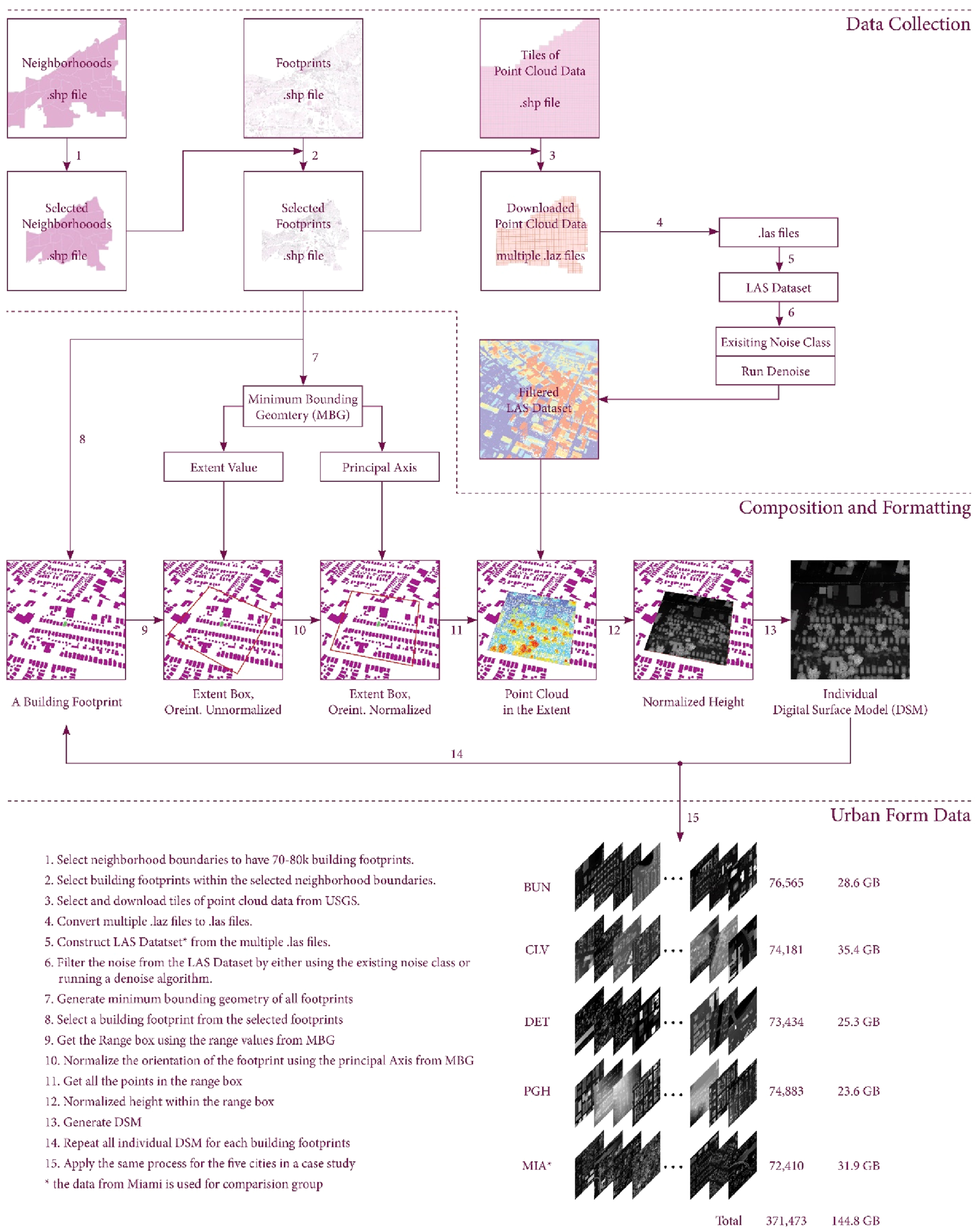

Only the buildings within these chosen neighborhoods are carefully filtered and utilized for data construction (step 2 in Figure 1). Specifically, Cleveland comprises 74,181 buildings, Detroit 73,434, Pittsburgh 74,883. I also collected data for Miami, comprising 72,410 buildings, serving as a comparison group representing the Sun Belt cities’ different urban culture. To train a deep learning model with large, diverse datasets, additional data from Buffalo, totaling 76,565 buildings, is collected.

Composition and formatting

The next step uses airborne LiDAR data and building footprints to create a new dataset in the desired format.

The initial task is to determine the extent of the neighboring urban space around a building. A narrow extent captures only building details, while a wide range includes comprehensive urban space, diminishing building significance and obscuring their interplay with the urban context.

The extent range for each building is based on its longest side, determined by using rectangular Minimum Bounding Geometry (MBG). A 50-foot unit is adopted, covering a minimum of 10 buildings (500 feet) and a maximum of 20 buildings (1000 feet), with each building centrally positioned within this range to determine the neighboring urban space.

In the composition process, the orientation of extents is normalized by rotating them to align with the depth axes of a building’s rectangular MBG, ensuring consistent morphological analysis across different cities Rhee and Krishnamurti (2023). This alignment is crucial for deep learning models studying urban form, allowing them to capture consistent features regardless of topographical variations. Height information from LiDAR data is also normalized for individual buildings to address discrepancies, with the lowest regions represented in black and the highest in white, accounting for local topographic changes.

The normalized LiDAR point cloud within a designated extent is transformed and saved as a 2000 by 2000 pixel image file, with height values represented by colors, maintaining 3D data in a 2D format. This ensures a consistent depiction of point cloud data, as shown in Figure 2.

Figure 2.

2D images with height information from point clouds (left) and reconstructed 3D (right).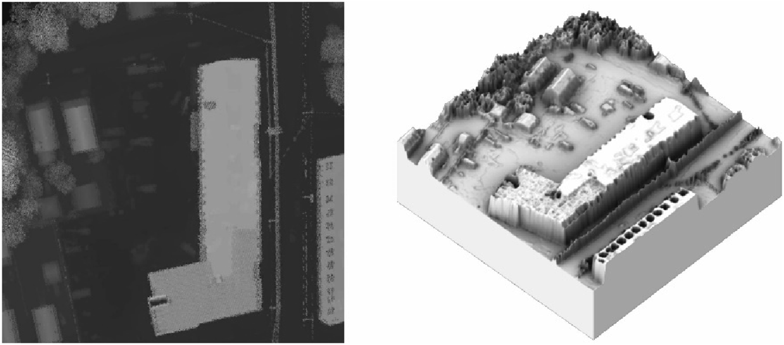

The process of composing and formatting the data is iteratively performed for each selected building in every city, resulting in the creation of a curated urban form dataset. Consequently, the number of data samples for each city corresponds to the number of selected buildings in that city, a total of 371,473 urban form data samples.

Clustering

To achieve clustering and identify distinct groups from the dataset, I first trained a type of Variational Autoencoder (VAE) model known as VQ-VAE Razavi (2019). While various machine learning models were considered, the complexity of the proposed urban form dataset necessitated a deep learning approach, with the VAE chosen for its ability to effectively capture data features. The VQ-VAE, in particular, excels in feature extraction through its use of vector quantization techniques Linde (1980) in image data. This model further facilitates qualitative performance evaluation by enabling the analysis of both reconstructions and extracted features.

Out of 371,473 total samples, 5000 were allocated for validation, 1000 for testing, and 366,473 for training. The dataset was augmented by creating mirror images through vertical and horizontal flipping, effectively quadrupling the training data volume. Figure 3 shows the training results, where the loss significantly decreases up to 1450 iterations and stabilizes around 0.001, correlating with improved reconstruction quality. By 1350 iterations, reconstructions achieve high quality, with shapes becoming distinguishable around 850 iterations and detailed patterns emerging by 1150 iterations.

Figure 3.

(Top): The first column displays ground truth images, and the second column shows reconstructed images, and graphs depicting training and validation loss (bottom).

The trained model captures latent vectors, which shape is (294,908, 64, 64), representing the features of the urban form dataset from the selected four cities. These vectors are subsequently flattened into (294,908, 4096) vectors for further analysis. K-Means clustering is then applied to this flattened vector space. Although alternative clustering methods, such as Gaussian Mixture Models (GMMs), DBSCAN (Density-Based Spatial Clustering of Applications with Noise), Spectral Clustering, and Self-Organizing Maps (SOMs), could be considered, the size of the feature vectors—approximately 9 GB—and the available computing performance made K-Means a more practical choice. For instance, while K-Means required approximately 4 hours to complete, DBSCAN took 8–10 hours depending on the parameters, significantly limiting the ability to conduct experiments with a variety of parameter settings.

In K-Means clustering, the number of clusters (N) is a critical parameter that dictates the classification of the dataset into N distinct groups. Increasing N results in more clusters, while decreasing N yields fewer clusters. For this study, which investigates various urban space types, an excessively high number of clusters complicates analysis, whereas too few clusters diminish its meaningfulness. Assuming approximately 10 urban form types per city, N is set to10. ¹

The results of this clustering analysis can be projected onto a map, offering insights into the types of urban spaces associated with each building in the city Rhee (2022). Figure 4 presents the mapping results for the four cities. These maps illustrate not only the morphological characteristics of individual buildings but also the relationships between building forms and their surrounding urban spaces. Buildings of the same color may share similarities in architectural forms, with their primary commonalities residing in the characteristics of the neighboring urban spaces.

Figure 4.

Clustering results projected onto building footprint map: Clockwise from top left, Cleveland, Detroit, Pittsburgh, and Miami. Refer to Figure S1 for more details.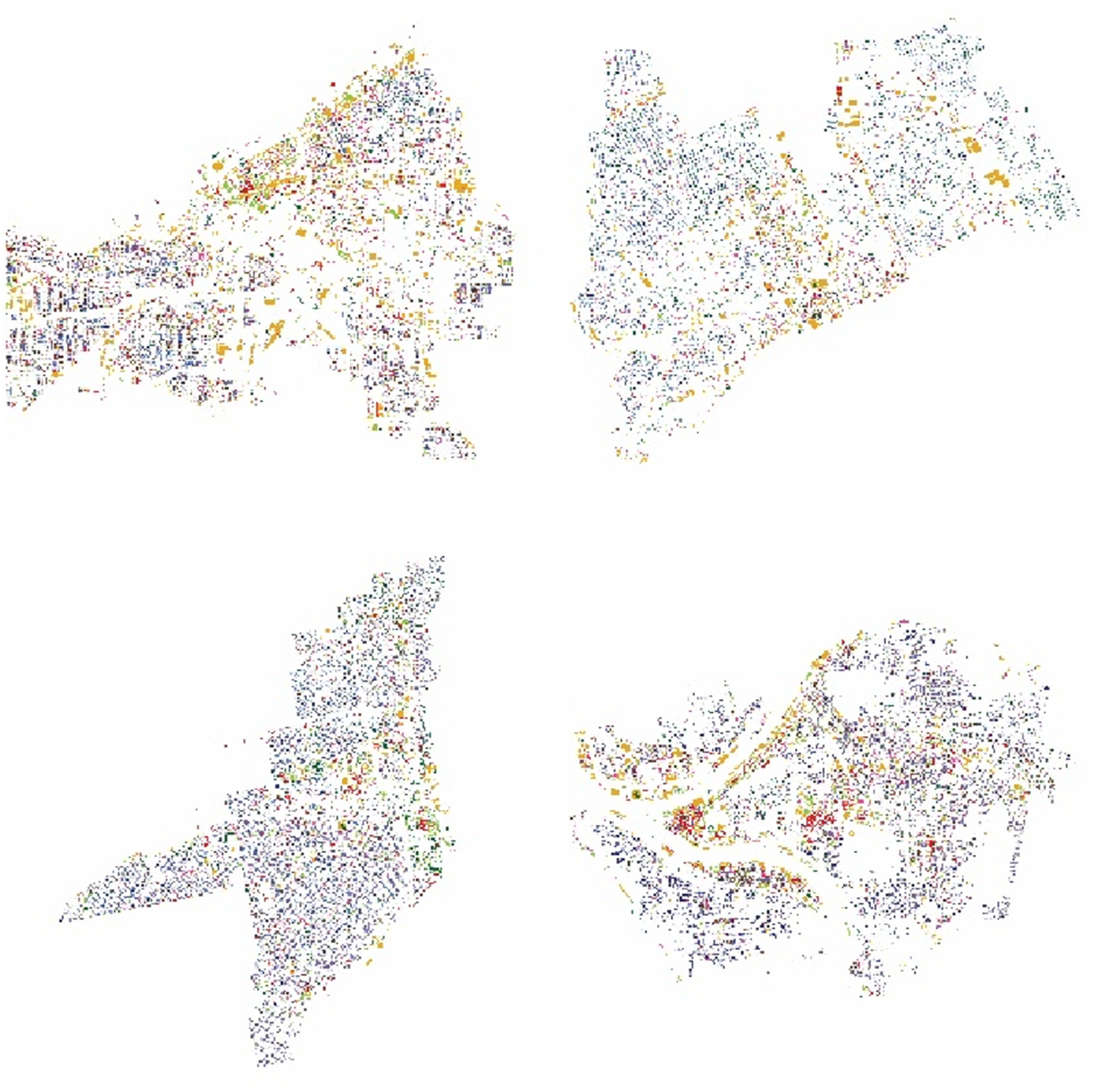

Urban structure

I regard cluster classes as urban form types and analyze their characteristics through basic statistics, representative forms, and features to derive a taxonomy of these types. This taxonomy enables geospatial analysis to reveal the distribution of each type across cities and their formation of cohesive fabrics, which in turn elucidates urban structure.

Basic statistics

The basic statistical analysis identifies variations in building area across different urban form types. Medium-sized buildings (Types 0 and 2) are prevalent in Miami and Pittsburgh, while smaller structures (Types 1, 3, and 5) show higher average areas in Cleveland. Monumental buildings (Type 4) are notably larger in Detroit and Miami. Medium-sized buildings (Types 6 and 7) are common in Miami, and small to medium-sized structures (Types 8 and 9) show modest variances across cities. This categorization into small, medium, and large buildings reveals distinct urban significances (see Figure S2 for more details.)

In terms of height, buildings in Types 0, 2, 4, and 7 are typically 3 to 5 stories, excluding Miami. Types 1, 3, 5, and 8 mostly consist of 2 to 3-story buildings, with lower heights in Miami. Miami predominantly features 1 to 2-story buildings, except for Type 6, which includes high-rises in Miami and Pittsburgh. Type 9 consists of one-story buildings across all cities, distinguishing it as a separate group based on height. This analysis highlights Miami’s unique architectural profile with notably lower buildings, except for high-rise Type 6 (see Figure S3 for more details.)

The distribution of building types varies significantly among cities. Cleveland has a high prevalence of Type 8, followed by Types 1 and 9, with Types 4 and 6 being less common. Detroit is dominated by Type 6, with significant occurrences of Types 3 and 5, and fewer small one-story structures (Type 9). Miami has the highest occurrences of Types 1 and 9, with fewer larger structures (Type 4). Pittsburgh shows high occurrences of Types 1 and 3, with fewer medium-sized buildings (see Figure S4 for more details.)

In summary, a quantitative analysis of the area and height of building types, coupled with their occurrences in each city, sheds light on the prevalence of various urban spaces centered around specific types of buildings. However, it should be noted that such quantitative analysis has its limitations, as qualitative aspects such as the conspicuous occurrences of Type 6 and 8 in specific cities, or relationships between Type 9 and Types 1, 3, and 5, may not be fully understood. Therefore, another investigation into the qualitative attributes of urban spaces in each city will provide a more accurate understanding of the distinctive characteristics of each type.

Representative form

Random sampling data (Figure S5) can validate inferences made from quantitative analyses. Urban Types 0, 2, 6, and 7 exhibit resemblances in terms of mid-sized building dimensions. Within Urban Type 0, there exists a recurring presence of mid-sized buildings that pervade the urban expanse. Conversely, Urban Type 2 manifests as an external domain encompassing solitary medium-sized buildings. In contrast to Urban Types 0, 2, and 7, Urban Type 6 demonstrates a propensity for substantiating a notably expansive encompassing void. In the context of Urban Type 7, small buildings conspicuously adorn the vicinity of substantial edifices with notable frequency.

However, the current sampling methodology limits a thorough qualitative assessment of each Urban Type’s distinctive attributes. Therefore, “representative forms” are devised using latent vectors from the trained model’s encoder to encapsulate the spatial configuration of each type. These representative forms, approximating the mean morphological attributes, facilitate a comprehensive analysis of each type’s spatial traits (Figure 5).

Figure 5.

Representative forms of each city by types.

Urban Type 0 predominantly features mid-sized buildings often grouped in configurations of 4–5 similar structures. These clusters may form linear arrangements along thoroughfares or compact clusters, primarily comprising downtown mid-rise edifices or commercial buildings within retail or office districts. Urban Type 1, on the other hand, manifests as a horizontal alignment of 2–3 rows of rectangular houses, stretching contiguously along streets and forming elongated urban spaces. This type typically encompasses suburban or habitation-oriented locales, with variations between Miami and Rust Belt cities in terms of building form and roof shape.

Urban Type 2 reveals slightly larger standalone buildings creating expansive independent spaces, unlike the clustered formations of Urban Type 0. These spaces often surround monumental buildings such as malls, offices, and institutes, with notable differences between Miami and Rust Belt cities in the prevalence of medium to large structures. Urban Type 3, similar to Type 1, features a bipartite or tripartite horizontal alignment of rectangular houses, but with shallower depths and less uniform interspacing. This type exhibits significant topographical variations, particularly in Pittsburgh, which are less evident in other cities.

Urban Type 4 comprises the surroundings of large edifices with marginal urban space, distinguishing itself with substantial structures, particularly in Rust Belt cities where industrial establishments are prevalent. Conversely, Urban Type 5, like Types 1 and 3, displays a horizontal arrangement of houses but with less distinct patterns due to abundant greenery and non-residential structures. This type reflects subtle deviations in a linear urban configuration, with notable differences between Miami and Rust Belt cities in terms of building height and roof shape.

Urban Type 6 is characterized by expansive independent urban spaces surrounding smaller buildings, often resulting from vacated surroundings of Types 0 or 2 structures. This type is prevalent in Detroit, where substantial vacant lots are common, but rare in Miami. Urban Type 7 blends medium to large structures with housing rows, incorporating elements of Types 2, 6, 1, 3, and 5, and frequently includes residential amenities like churches and schools. Urban Type 8 features a vertical arrangement of rectangular houses in a square-like configuration, prevalent in Cleveland. Lastly, Urban Type 9 characterizes urban spaces around small buildings, distinguished by non-linear central structures, often associated with garages and warehouses, reflecting interrelationships with Types 1, 3, and 5.

Feature analysis

For a more intricate analysis of the distinctive attributes across each urban type, an examination of features becomes crucial. Here, “features” refer to the latent vectors extracted by the encoder of the VQ-VAE model. By inputting the data into the encoder, which has been trained on the training dataset, the corresponding latent vectors can be extracted.

Since representative form, sampling, and mean feature analysis are visually based, further quantitative analysis is needed to validate urban type similarities. The Structural Similarity Index (SSIM) was used to quantify inter-type similarities, considering luminance, contrast, and structure for a detailed assessment. The results, presented in Figure S6, show higher similarity among Types 0, 2, and 4, as well as among Types 1, 3, and 5. Type 6 shows higher similarity with Types 2 and 3, while Types 7, 8, and 9 exhibit notable similarities, particularly Type 7 with Types 2, 3, and 4. These findings broadly classify the types into four groups: Types 0, 2, and 4; Types 1, 3, and 5; Types 7, 8, and 9; and Type 6, which does not align distinctly with any group.

Figure 6 illustrates the visualization of mean features for each urban type using the average vector of extracted latent vectors, with annotations of corresponding morphological traits. In this visualization, bright areas represent elevated regions, while dark areas indicate lower elevations. Urban Type 0’s mean feature shows a vivid hue at the center with lighter hues and darker shades around it. Urban Type 1 displays bright patterns forming three horizontal linear arrangements, while Urban Type 2’s mean feature appears as a singular elongated mass oriented vertically. Urban Type 3 features luminous patterns forming two horizontal linear arrangements at the top of the area. Urban Type 4’s mean feature is mostly luminous, and Urban Type 5 shows two horizontal linear arrangements of luminous patterns at the bottom.

Figure 6.

Visualization of mean features for each urban form type with annotated morphological traits.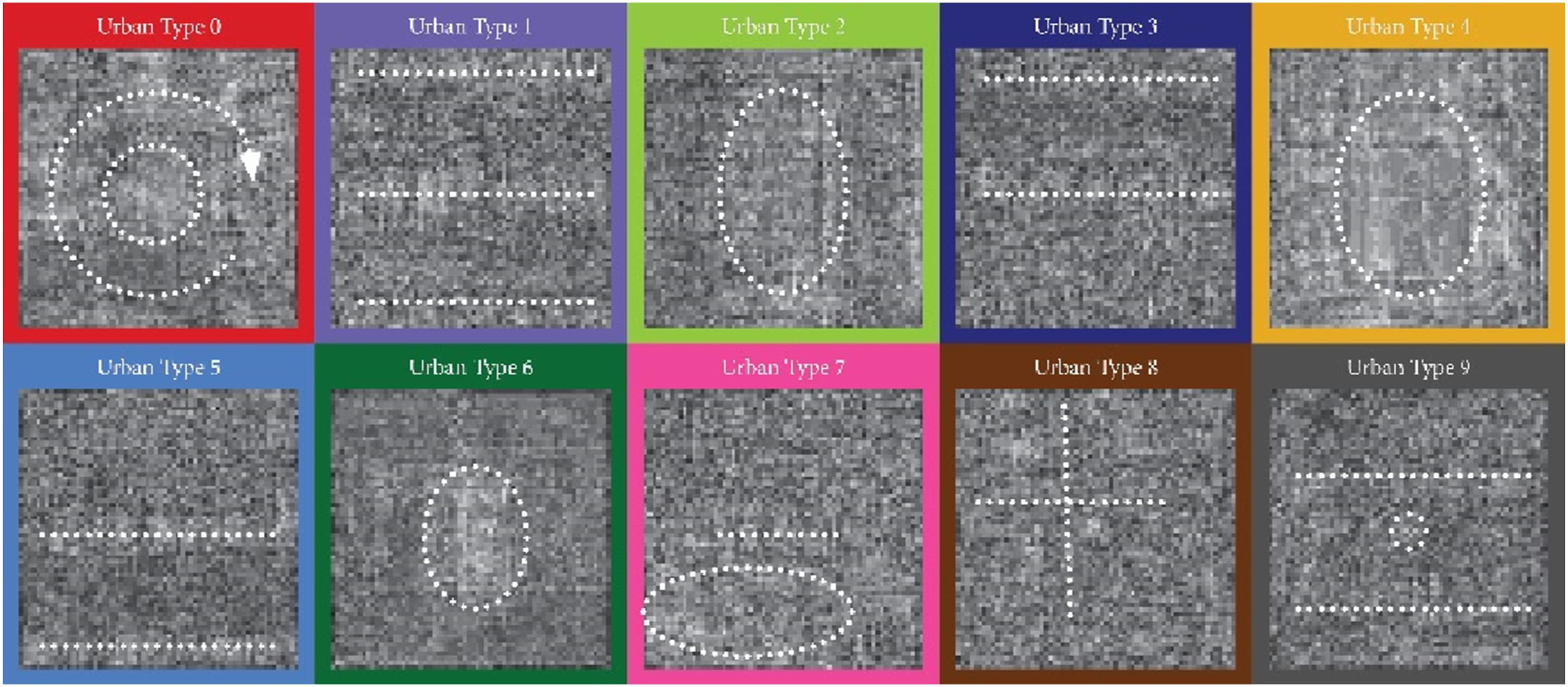

Urban Type 6 is characterized by a prominent white cluster at the center, surrounded by darker tones at the periphery. Urban Type 7’s mean feature shows a faint linear pattern at the center with a luminous cluster in the lower-left quadrant. Urban Type 8 has a darkened motif forming a slightly skewed cross shape from the center to the upper left corner. Lastly, Urban Type 9 features a small bright cluster at the center, with faint linear bright patterns above and below it.

Feature visualization and mean feature analysis confirm two main insights. First, the classification of Types 0, 2, and 6 with bright central regions and Types 1, 3, and 5 with horizontal linear patterns is validated. Second, qualitative inferences for Types 4, 7, and 9 are supported, while Type 8 shows a cross-shaped form, indicating a more diverse range of urban forms than previously identified.

Taxonomy

Based on building height and footprint area, representative forms, mean features, and feature similarity, urban types were classified, culminating in a taxonomy (see Table 1). The classifications are labeled “C” for “Central,” “L” for “Linear,” and “M” for “Miscellaneous,” independent of the other categories. The final classification for each urban type is determined by the most frequently occurring label in each category.

Table 1.

The results of grouping by different analyses: Building height and footprint area, representative form, mean features, and feature similarity.

Type	0	1	2	3	4	5	6	7	8	9
Area	C	L	C	L	M	L	C	C	L	M
Height	C	L	C	L	C	L	M	L	L	M
Rep.form	C	L	C	L	C	L	C	M	L	M
Mean feat	C	L	C	L	C	L	C	M	M	M
Feat. similarity	C	L	C	L	C	L	M	M	M	M
Final class	C	L	C	L	C	L	C	M	L	M

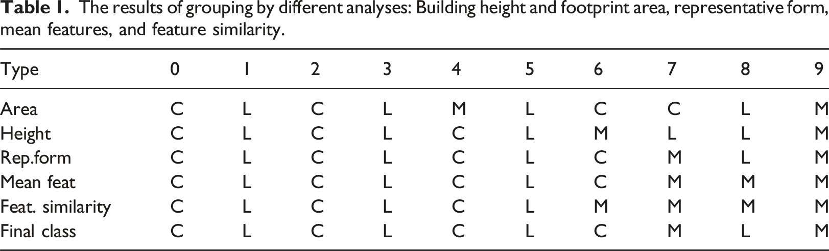
Urban Types 0 and 2 are central spaces with surrounding areas, consistently classified as such. Types 1, 3, and 5 display linear patterns, while Type 4, initially classified as “M” for its area, is ultimately “C.” Type 6, deviating in height and feature similarity, is “M.” Type 7 shows both central and linear traits but is “M” due to distinct features. Type 8 is linear, similar to Types 1, 3, and 5, while Type 9, with unique traits, is “M.” Thus, Types 0, 2, 4, and 6 are “C” (Central), Types 1, 3, 5, and 8 are “L” (Linear), and Types 7 and 9 are “Hybrid.” Figure S7 illustrates this taxonomy, categorizing forms into Central, Linear, and Hybrid groups, with further subgroups based on spatial occupancy and row orientation, highlighting the predominance of morphological traits and vertical arrangements.

Urban fabric maps

Mapping the taxonomy of urban types onto geospatial data reveals their distribution across cities, illustrating the urban fabric and structure. I define urban fabrics as the boundaries of urban spaces formed by clusters of the same urban form type. The centroids’ coordinates of each building footprint are aligned along the X-axis of the input data, while urban type labels are assigned to the Y-axis. This data is then inputted into a KNN classifier for clustering analysis.

Several key points emerge from this map (Figure 7). Firstly, the colors representing fabric types are unrelated to land use planning, zoning, or functions. For instance, a green patch signifies an area corresponding to Urban Type 6 fabric, not a park or wooded area. Additionally, the map is based on building footprints and does not account for land programming like parks, water, or hills. Thus, if a single building within a park is classified as Urban Type 6, a large portion of the park may be represented as such. Therefore, it is crucial to consider the granularity of fabrics and not assume that larger areas are always dominant, referencing the building footprint map for accurate interpretation.

Figure 7.

Color-coded urban fabric maps: Clockwise from top left, Cleveland, Detroit, Pittsburgh, and Miami. Refer to Figure S8 for more details.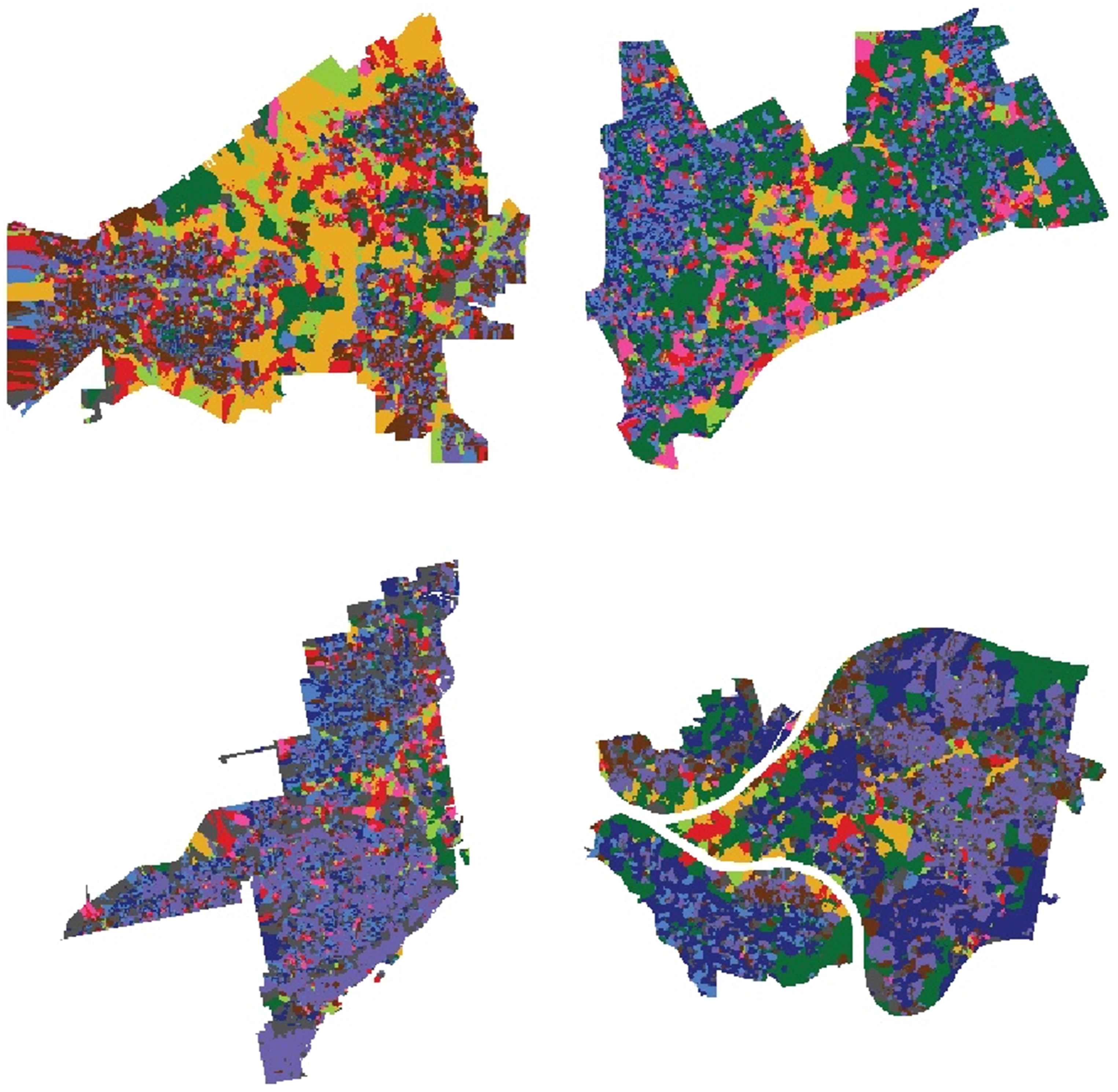

Based on the analyses above and observation on the fabric maps, Figure 8 presents a diagram illustrating common urban structure among the three Rust Belt cities, distinguishing them from such structure in Miami.

Figure 8.

A common urban structure shared among the three Rust Belt cities (left), distinguished from such structure in Miami (right).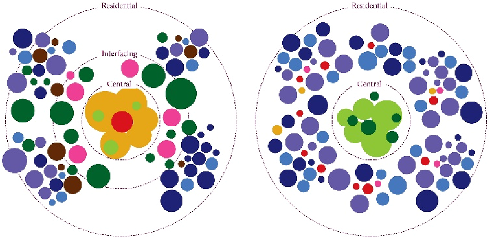

Results

Rust Belt cities and Miami exhibit notable differences in Urban Types 4. In Rust Belt cities, Urban Type 4 fabrics predominantly emerge near downtown areas, often collaged with Urban Types 0, 2, 6, and 7. In contrast, Miami’s downtown is primarily characterized by Urban Type 2 (vacant spaces around high-rises) and Urban Type 6, with modest quantities of Urban Type 4. Rust Belt cities consistently feature substantial areas of Urban Types 0 and 2 near downtowns, forming clusters of mid-sized buildings surrounded by larger structures, indicative of urban spaces formed within the interstices of 4–5 story building clusters.

At the periphery of these collages in Rust Belt cities, smaller granular fabrics of Urban Types 1, 3, 5, and 8 are observed, often buffered by Types 6 or 7. In contrast, Miami exhibits direct interactions between large buildings or mid-rise clusters and residential fabrics, with less evidence of buffering by Types 6 or 7. Urban Type 6 represents independent buildings within vacant urban spaces, while Urban Type 7 blends mid-sized buildings with rows of houses. These spatial characteristics highlight how Rust Belt cities integrate large structures with smaller residential spaces through either open spaces or blended fabrics, contrasting with Miami’s more direct interfacing of urban forms.

The subsequent notable aspect is the distribution of Urban Type 6 which exhibits varied distributions across Rust Belt cities and Miami. Detroit has the highest quantity and largest fabric sizes of Urban Type 6, broadly distributed throughout the city. Pittsburgh follows with a significant but less extensive distribution compared to Detroit, while Cleveland and Miami show smaller, more fragmented distributions. In Detroit, Urban Type 6 often comprises smaller independent structures surrounded by vacant spaces, suggesting alignment with high-vacant-lot areas (Figure S9 in Supplementary Material.) Observing the footprint with this fabric map, most Urban Type 6 fabrics in Detroit seem originally aligned with rows of houses, but it is inferred that they now represent buildings with independent urban spaces due to the increase in vacant lots. Based on this inference, when overlaying the location of high-vacant-lot areas on the Census map with the Urban Type 6 fabrics map in Detroit, a significant alignment can be noticed (Figure S10 in Supplementary Material.) This suggests that many Urban Type 6 fabrics in Detroit can be understood as the spatial configuration of buildings with surrounding vacant spaces due to vacant lots. Cleveland and Pittsburgh also feature Urban Type 6 fabrics centered around medium-sized structures, with some areas showing similar vacant-lot patterns as Detroit. Miami, however, displays the lowest quantity of Urban Type 6, mainly concentrated in downtown areas.

In Cleveland and Pittsburgh, Urban Type 6 buildings are scattered with wide vacant spaces between rows, transitioning linear urban spaces into more central configurations. This transformation differentiates these spaces from densely packed areas, suggesting an increase in vacant spaces leads to the formation of independent structures. Miami’s Urban Type 6 buildings are taller, often appearing as podiums for high-rises, surrounded by lower structures. This classification is distinct from the vacant-lot fabrics around residential structures in Detroit and more similar to the downtown configurations in Cleveland and Pittsburgh.

These characteristics are well reflected in the schematic urban structures, with the three Rust Belt cities exhibiting three main urban structural features.

Firstly, in the three Rust Belt cities, urban structure includes an Urban Type 0 fabric, denoting interstices yielded by clusters of 4–5 story medium-sized buildings in proximity to downtown areas. Conspicuously surrounding this is the Urban Type 4 fabric composed of large buildings. Intermittently interspersed between these fabrics is Urban Type 2, signifying the external spaces of mid- or high-rise structures. This combination of Types 0, 2, and 4 is termed as central fabrics.

Secondly, Urban Types 1, 3, 5, and 8, constituting residential fabrics encircling the central fabrics, manifest collectively. These residential fabrics exhibit a higher level of granularity compared to the central fabrics, shaping a linear urban space primarily characterized by rows of houses. Vacant lots attributed to Urban Type 6 occasionally can undermine this linearity.

Lastly, when central fabrics interface with residential fabrics, they often utilize fabrics primarily characterized by empty spaces, such as Urban Type 6, or fabrics where linear and central urban spaces blend, like Urban Type 7, as buffers. These are referred to as interfacing fabrics.

In the case of Miami, it shares similarities with Rust Belt cities in possessing central and residential fabrics. However, in its central fabrics, Urban Type 4 is absent, and Urban Type 2 predominates. Urban Type 6, representing expansive external spaces around independent structures, sporadically intervenes within Urban Type 2 fabrics. Central fabrics directly about residential fabrics without interfacing fabrics. Within the residential fabrics, fabrics corresponding to Urban Type 0 or 7 form functional sub-centers that support residential fabrics, occasionally even incorporating large buildings corresponding to Urban Type 4.

In summary, the key findings are as follows:

• Rust Belt Cities: Characterized by 4–5 story buildings near downtown, surrounded by larger buildings and interspersed with mid- or high-rise structures, creating a mix of central and residential fabrics. Vacant lots occasionally disrupt linearity.

• Miami’s Distinct Fabrics: Shares some characteristics with the Rust Belt cities but lacks large building fabrics in its central areas. Its urban structure is dominated by mid- or high-rise external spaces.

• Structural Integration in Miami: Unlike the Rust Belt cities, Miami’s central and residential fabrics merge directly, forming sub-centers within residential areas, sometimes featuring large buildings.

• Key Contrast: The Rust Belt cities showcase an interconnected mix of downtown and residential areas linked by large edifices or vacant lots, while Miami exhibits a more distinct separation between its downtown and residential regions.

Conclusion

I proposed a comparative computational methodological framework to investigate the common urban structures of Rust Belt cities, focusing on the typo-morphological characteristics of urban space. This approach includes the construction and processing of a novel urban dataset. This framework uses a specific data scheme to define individual urban spaces, creating a dataset centered on a single building that includes its neighboring urban spaces within a certain extent. A deep learning model was then employed to capture the morphological features of these urban spaces, clustering them to identify types of urban spaces and leveraging the form data to reveal their morphological characteristics. Analyzing these characteristics allowed for delineation of urban fabric patterns and investigation of the unique urban structures of the three Rust Belt cities.

This analysis reveals two key spatial characteristics of Rust Belt cities. Firstly, the urban spaces of massive industrial facility buildings show similar spatial configurations across these cities. Secondly, there are empty lots and mixed or hybrid programs connecting downtown and residential fabrics. While restructuring to downsize the overall scale of the city is important, this analysis highlights the need to incisively renovate spaces that embody the unique characteristics of Rust Belt cities. The large lots surrounding these massive buildings have the potential to be transformed into publicly developed spaces or facilities for the large public. This renovation offers several benefits: it can occur on the outskirts of residential areas without encroaching on citizens’ living spaces, it is located between downtown and residential areas, providing high accessibility, and it already has extensive infrastructure from its industrial past.

This renovation can also be associated with the potential of surrounding empty lots. Extensive empty lots can be incorporated into this renovation process, while scattered empty lots can be revamped by changing zoning regulations to introduce new programs considering the renovation. As the value of surrounding areas increases due to development, private development on vacant land could also be encouraged. This approach to renovation can help mitigate the pervasive issue of empty lots in Rust Belt cities, preventing their spread and contributing to urban revitalization.

While this research contributes significant insights into the urban structure of the Rust Belt cities through the proposed computational method, it is important to acknowledge its limitations.

First, a systematic evaluation of this method is necessary. Several approaches can be taken. One approach is to validate the method by incorporating existing urban form and structure analysis and comparing the results. This not only demonstrates the method’s reasonableness and validity but also highlights its potential to provide new insights distinct from existing methods. Another approach is a site survey. As one of the best ways to verify data generated from computer analysis, conducting a site survey can effectively assess how well the nuanced classifications produced by this method align with real-world conditions.

Additionally, the scope of data units relating to adjacent urban spaces represents a pivotal yet challenging facet requiring in-depth investigation. This aspect has been pinpointed as a significant research gap and a direction for future inquiry, particularly highlighted in interviews with urban planners. The task extends beyond the mere technical demarcation of these ranges; it necessitates a nuanced understanding of their urban implications. For example, a 50 m range may only capture the area directly surrounding a building, while a 500 m range could encompass a whole neighborhood. It is important to conduct comprehensive experiments to discern how varying these ranges influence the accuracy and relevance of type identification outcomes.

Lastly, future research should aim to develop deep learning models that integrate morphology feature extraction and clustering. The current methodological framework utilizes separate models for these tasks, which can independently introduce errors. Even if there are no errors in the deep learning phase, clustering can introduce a different type of error, making it challenging to manage errors in an integrated manner. This separation complicates the reduction and management of errors across the classification process. If a single deep learning model performs both morphology feature extraction and unsupervised clustering, errors occurring during the training process would be integrated across the entire classification, potentially leading to higher classification accuracy. This integrated approach could streamline error management, enhancing the overall effectiveness of urban structure analysis.

Supplemental Material

Supplemental Material - Comparative Analysis of Urban Structures in Three American Rust Belt Cities

Supplemental Material for Comparative Analysis of Urban Structures in Three American Rust Belt Cities by Jinmo Rhee in Environment and Planning B: Urban Analytics and City Science