Sage Journals: Discover world-class research

Abstract

Quantifying, understanding and predicting the number of pedestrians that are likely be present in a particular place and time (‘footfall’) is critical for many academic, business and policy questions. However, limited data availability and complexities in the behaviour of the underlying pedestrian ‘system’ make it extremely difficult to accurately model footfall. This paper presents a machine learning model that is trained on a combination of hourly footfall count data from sensors across a city as well as important contextual factors that are associated with pedestrian movements such as the structure of the built environment and local weather conditions. The aims are to better understand the relationship between various contextual factors and footfall and to predict footfall volumes across a spatially heterogeneous city. The case study area is the city of Melbourne, Australia, where abundant pedestrian count data exist. Time-related variables, particularly time-of-day and day-of-week, emerged as the most significant predictors. While some built environment factors such as the presence of certain landmarks and weather conditions were influential, they were less so than temporal cycles. Interestingly the model over-estimates footfall in the years following the COVID-19 pandemic, suggesting that urban dynamics have yet to return to pre-pandemic levels (and may never do). The paper also demonstrates how the model can be used to assess the impacts that large events have had on footfall, which has implications for policy makers as they try to encourage foot traffic back into city centres.

Keywords

Machine learning urban analytics random forest footfall pedestrian dynamics modelling

Introduction

By 2050, two out of every three people are likely to be living in cities (United Nations, Department of Economic and Social Affairs, Population Division, 2018). This represents an unprecedented transition from humans living in rural areas to urban areas. This seismic shift makes it ever more important to improve our understanding of the factors that drive people’s movements around cities and to develop tools that will offer predictions of up-to-date urban dynamics.

One important area in the study of urban dynamics is that of the ambient (Malleson and Andresen, 2016), or ‘temporary’ (Panczak et al., 2020), population. The ambient population is defined as the population who are ‘within a given geographical area at a specific point in time, excluding individuals at their place of residence and those utilising modes of transport’ (Whipp et al., 2021b). It includes commuters, shoppers, tourists, event-attendees and more, and thus extends the scope of a city beyond the ‘classical’ residential population. It is an extraordinarily dynamic object of study because it constantly changes with external factors such as the weather or time of the day, yet at the same time it influences (and is influenced by) the shape of a city. For example, the ambient population directly determines the extent of traffic flows, litter and economic activity, to name just a few, and thereby indirectly affects all risks and benefits associated with the dense and complex living conditions within a city.

Despite the importance of the dynamics of the ambient population, it can be extremely difficult to analyse its size and characteristics. There are two main reasons for this. Firstly, unlike with residential populations, where national population censuses and other administrative datasets or household surveys provide rich and accurate information, the availability of information about ambient populations is much more sparse. Secondly, the relationship between the urban environment and the behaviour of the ambient population is difficult to model as many (inter)relationships between variables may be non-linear. For example, a narrow, historical street may deter pedestrians during weekdays as people use main thoroughfares to move quickly between activities, but may attract people at weekends when they might like to spend time exploring the more unusual/interesting parts of a city.

In this paper, we apply random forest regression and gradient boosted decision trees that are able to capture highly non-linear dynamics. We do this to (i) better understand the impact that the built environment and other contextual factors will have on the number of pedestrians and (ii) to predict the size of the pedestrian population under different conditions with the help of real-time information from city sensors. The case study area is the city of Melbourne, Australia, where abundant pedestrian data exist thanks to a large number of sensors that have been installed by the local government and reported on a publicly available open data portal.

The main findings are: (i) the random forest regressor provides more accurate predictions than the gradient boosted decision trees; (ii) the model found it harder to accurately predict footfall at night and in certain places that had sporadic footfall patterns caused by their proximity to major attractions; (iii) time-related variables like the time-of-day and day-of-week were by far the most important predictors of footfall; (iv) some built environment factors were also found to be important, especially distance to the city centre and presence of certain landmarks, but overall the built environment was less influential than temporal cycles; (v) the model over-predicted footfall in the years after the pandemic, suggesting that even though some footfall has recovered the dynamics are still fundamentally different compared to pre-pandemic; (vi) the model is able to provide insights into the change in footfall caused by extraordinary events, beyond those that would be expected given the particular conditions on the day.

Beyond its practical applications, the work also contributes to theoretical frameworks in urban geography. By quantifying how granular spatial variables influence the ambient population, we provide empirical support for pedestrian movement theories such as the social force model, highlighting the role of external forces – like urban features and landmarks – in shaping pedestrian flows. Our data-driven approach operationalises concepts from Time Geography by identifying specific spatio-temporal constraints that impact human movement, thus making abstract theoretical ideas more concrete and quantifiable.

We will discuss the data and methods employed in sections 3 and 4, respectively, with preliminary results presented in Section 5, contributions of the empirical work to underlying theory are outlined in Section 6, limitations discussed in Section 7, and conclusions drawn in Section 8. The following Section, 2, contextualises the study.

Background

Understanding and quantifying the ambient population is important for numerous practical reasons and can generate novel insights relating to several theoretical frameworks in geography. The implications for theoretical work in geography in urban studies we discuss in Section 6. In urban planning, understanding the ambient population allows for the design of infrastructure to accommodate the projected footfall, allowing cities to ensure effective functionality. Hence, the ambient population has been studied to determine the need for pedestrian paths, bicycle lanes and public transportation services (Crols and Malleson, 2019; Cooper et al., 2021). From an economic perspective, it can help businesses to determine where to locate their operations. For instance, retail businesses often prioritise stores in high footfall streets to maximize exposure and sales. From an environmental perspective, footfall has been studied in relation to exposure to particulate matter and other pollutants in the air (Guo et al., 2020; Park and Kwan, 2017; Picornell et al., 2019) and in relation to noise levels and subsequent adverse health effects (Moudon, 2009). The most common application that motivates the estimation of the ambient population is that of crime analysis (Andresen, 2006, 2011; Andresen et al., 2012; Bogomolov et al., 2014; Traunmueller et al., 2014; Felson and Boivin, 2015; Malleson and Andresen, 2015a, 2015b; Boivin and Felson, 2017; Hanaoka, 2018; Hipp et al., 2019; Liu et al., 2022; Gu et al., 2023; Song et al., 2023) where it has been long recognised that to properly estimate crime rates it is necessary, for some crime types, to estimate the non-residential population of potential victims as the rate denominator. More recently, the quantification of the ambient population has also started to motivate research into population segregation (Candipan et al., 2021; Gu et al., 2023), human activities (Martin et al., 2015; Zheng et al., 2023) and crowd flows (Botta et al., 2015).

Given the diversity in applications, it is not surprising that there is similar diversity in the data sources used. Early work used Land Scan satellite imagary data (Andresen, 2006), although the resolution of these data proved too coarse for fine-grained analysis. The proliferation of mobile phones among populations has made telecommunications data – SMS, calls, data transfer or even the locations of cell towers themselves (Johnson et al., 2020) – a rich source for information about peoples’ locations (Bogomolov et al., 2014; Botta et al., 2015; Hanaoka, 2018; Song et al., 2023; Traunmueller et al., 2014), albeit one that is privately owned and usually extremely difficult and/or expensive to access for research. Smartphone applications that collect users’ GPS locations are potentially useful (e.g. see Gu et al., 2023), but as well as being prohibitively costly, such data raise difficult questions of privacy and consent. A data type that has recently found some popularity for estimating pedestrian volumes is that of Street View Images (SVI); digital photographs taken at the street level and made available by companies such as Google and Baidu. Analysis of the objects present in images (e.g. clear sky, greenery and roads) can be linked to pedestrian counts data to identify correlations. For example, Chen et al. (2020, 2022) use Convolutional Neural Networks to quantify street scenes and use these metrics as inputs into a regression model with pedestrian counts (provided by Baidu AI) as the dependent variable. They find that features such as greenery, open sky and pavements are positively associated with pedestrian volumes. Perhaps the most commonly-used source is that of social media data, with Twitter being particularly popular (Malleson and Andresen, 2015a, 2015b; Botta et al., 2015; Hipp et al., 2019; Candipan et al., 2021; Liu et al., 2022), but these data have their own problems with bias and representation, and (as the Twitter Research API was closed in March 2023) with access. Finally there are examples of the use of surveys and administrative data (Boivin and Felson, 2017; Felson and Boivin, 2015; Martin et al., 2015). For example, Martin et al. (2015) propose a statistical framework for redistributing a residential population according to likely social and commuting flows coupled with significant points of interests (hospitals, employment centres, etc.).

With respect to the methods employed, most of the studies referred to have not explicitly attempted to develop measures of the ambient population in their own right. Rather they have collected data as potential proxies for the ambient population and then used models – typically logistic, (negative) binomial or linear regression, or techniques branded as ‘machine learning’ such as neural networks and random forests – to estimate the size of the relationship between the raw data and the phenomena of interest. Some, however, do attempt to refine the ‘raw’ data into a more robust population estimate. For example, Stefanidis et al. (2013) and Thakur et al. (2015) propose computational frameworks that are designed to consume and link ‘ambient geospatial information’ (Stefanidis et al., 2013) from diverse sources and subsequently infer information about ambient populations. Whilst such frameworks are important, they are of limited value here because they are predicated on access to streams of data from private companies (typically social media companies) that are not readily available. The aforementioned work by Martin et al. (2015) attempts to construct a holistic representation of the population from publicly available administrative data but is not used here because it relies on averaged temporal estimates so could not be used to quantify the population on specific days of the year. Whipp et al. (2021a) used geographically-weighted regression to estimate the size of the ambient populations, drawing on data with a temporal resolution of an hour, but only modelled two population groups (‘day time’ and ‘night time’).

Overall, despite a reasonable volume of research that attempts to explore the implications of the ambient population for a particular field (crime, mobility, etc.) there is relatively little work that attempts to create a robust representation of the population itself. In addition, those studies that do attempt to model the population do so at coarse spatial and temporal resolutions. This work makes an important contribution by drawing on high-resolution spatio-temporal data from a variety of sources and creating a model that can make predictions to the nearest hour at a fine spatial resolution.

Data preparation

Ambient population data: Footfall counts

Our case study area is the city of Melbourne, Australia. The city has abundant high-resolution data openly available at the City of Melbourne Open Data Portal (https://data.melbourne.vic.gov.au/pages/home/). This includes hourly counts of pedestrians and a wealth of useful information about the built environment that can be used to attempt to predict footfall. Here we use the footfall data to represent the ambient population. The data are generated from 82 sensors that are ‘typically installed under an awning or on a street pole to form a counting zone on the footpath below’ and record pedestrian ‘movements’, although the precise mechanism for detecting pedestrians is not stated (City of Melbourne Open Data Portal, 2023). Pedestrian counts are reported at the temporal resolution of 1 hour. Although some sensors were reporting as far back as 2011, many of the sensors were installed more recently. In addition, some sensors do not have full count information throughout their entire period of operation. Regarding the spatial configuration, broadly the sensors are located in the Melbourne’s Central Business District rather than being distributed across the wider urban region as a whole. Some neighbourhoods have been sensed for much longer periods than others and this will have implications on the generalisability of the work (some communities may not be as well represented as others) but we do not consider this potential bias here. There is no bias in the hours, days of week or month for which data are recorded. Figures S1 and S2 in the supplementary material illustrate these spatial and temporal patterns.

Explanatory variables

We attempt to build a model that can predict the variation in footfall counts (the dependent variable) from the patterns in a range of secondary data that are hypothesised to influence the dynamics of the ambient population.

The ambient population is understood to be responsive to characteristics at both micro- and macro-scales. At the macro-scale, the time-of-day and day-of-week, the prevailing weather conditions, economic and social conditions and occurrence of national holidays or special events will all influence urban footfall. Very high or low temperatures, rainfall and wind are all correlated with lower pedestrian volumes (Runa and Singleton, 2021). Conversely, bank – or other national or regional – holidays may elevate the ambient population (Trasberg et al., 2021). Evidence also indicates that features of the built environment at the micro-scale, within the immediate environment of a particular street, can be key drivers of the ambient population (Ewing et al., 2016). In particular, how individuals perceive the streetscape is thought to be governed partially by visually dominant features such as buildings and trees (Harvey et al., 2015), and by street furniture (including signs, benches, bins, and lights) which add complexity to the streetscape. The functionality, as well as form, of the environment is also of relevance, with Ewing et al. (2016) differentiating between the influence of active (shops, restaurants, parks, etc) and inactive (abandoned buildings, car parks, etc) land uses. Finally the socio-economic and/or demographic characteristics of the people who live in or visit an area may influence its footfall, so we include some additional aggregate census variables.

Temporal features

The time-of-day and day-of-week are likely to have a substantial impact on footfall counts. Representing these variables is complicated, however, as they are cyclical. If using a simple linear scale, then 23:59 and 00:00 would be treated as being a long way apart, even though they are separated by only 1 minute, as would Sunday and Monday (assuming Monday is day 0 and Sunday is day 6). Therefore, we apply a cyclical encoding and convert each variable into two separate features (Njilla et al., 2019). For the time-of-day these are Sin_time and Cos_time, calculated as sin(2πt/24) and cos(2πt/24), respectively, where t is the decimal time. For the day-of-week these are Cos_weekday_num and Sin_weekday_num calculated in a similar way.

Weather conditions

An obvious explanatory variable is the weather; in general, foot traffic will be lower on days with heavy rainfall or those that are especially hot or cold. We obtain historic weather data from the Melbourne weather service, including hourly temperature, humidity, pressure, wind speed and a binary measure of the presence of rainfall.

Common behavioural routines

Human mobility shows a strong degree of regularity, driven by shared behavioural routines such as ‘9-5’ employment, public holidays, and weekends. To capture these shared routines we extracted the day of week, week number, month, and season from the raw time of each pedestrian count record.

Built environment data

Relevant secondary data on the built environment are also available from the Melbourne Open Data Portal. We use the following to create explanatory features that are related to the built environment:

Pedestrian Footpath Network: we calculate the betweenness – a measure that is typically used in space syntax (Bafna, 2003) to quantify how well a link is connected to the wider network. In this case, for a network of roads and pedestrian footpaths, betweenness captures the level of connectivity for each road, hypothesising that better connected roads are likely to exhibit greater pedestrian traffic (Leccese et al., 2020);

Street Furniture: locations of benches, information pillars, litter bins, street lights, etc;

Buildings: locations, types and sizes of different buildings (residences, shops, hospitals, leisure establishments, etc.);

Landmarks: including places of worship and community centres.

In order to associate the sensors with the built environment data, a radius was drawn around each sensor. The optimal size of this radius was unknown so a variety of different buffer sizes were experimented with (see Section 4.2). Note that it is likely that the scale of influence of different features of the built environment may vary – for example, a railway station may influence footfall over a larger area than a street light – so future work will experiment with different buffer sizes for different features. For the following features, a count of the number of objects within each sensor radius was calculated: street furniture items; lights; buildings; and landmarks. For betweenness, the value of the footpath edge that was closest to the sensor was taken. The average number of floors within the sensor’s radius was also calculated and included as a variable. Figure S3 illustrates an example buffer region.

Socio-economic and demographic features

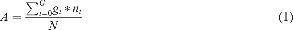
It is possible that socio-economic or demographic factors may also influence footfall counts in an area. However, quantifying such features is problematic. For example, although ‘night time’ residential data are readily available, for some factors it may be more appropriate to quantify the ‘ambient’ population – that is ‘the number of people within a given geographical area at a specific point in time, excluding individuals at their place of residence and those utilising modes of transport’ (Whipp et al., 2021b). In addition, many socio-economic and demographic features will be highly correlated to features of the built environment. The focus of this paper remains on built environment, time, and weather data, but we include the following key characteristics as they are arguably the most likely to influence footfall (recognising that mean values may not capture the distributions and hence the desired effects as effectively as using numerous distinct groupings, but we leave this for future work):

Mean age: The mean age of all residents, chosen because younger populations, such as students and young professionals, may be more likely to engage in walking for commuting and leisure (Lee et al., 2018). In the Australian census, age is provided as counts of people in different age groups so we calculate the mean age, A, for an area as:

A = \frac{\sum_{i = 0}^{G} g_{i} * n_{i}}{N}

(1)

where G is the total number of different age groups, g_i is the mode of age group i, n_i is the number of people in age group i and N is the total number of people in the area (the sum of the n_is).

Mean income: Lower-income individuals may rely more on walking due to limited access to costly public or private transport and also because income can influence the times at which journeys are made (Pucher and Renne, 2003). Income is also represented in the census by counts of people in different income bands and is therefore included using the same approach as equation (1).

Mean level of schooling reached: Included to capture the impacts of educational attainment on footfall behaviour, the census counts the number of people in each Highest Year of School Completed (HYSC) band so the mean band is calculated using the same approach as equation (1).

The data are obtained from the three most recent Australian censuses from 2011, 2016, and 2021 using the most granular geography, ‘SA1’, that produces areas that have, on average, 400 residents in each (ranging from 200 to 800). For each row in our data (an hourly count for a particular sensor) we attach the variable that corresponds to the closest census using the SA1 area that the sensor is located within.

‘Business as usual’ and outlier removal

When observing the footfall counts from individual sensors, it quickly becomes clear that most exhibit regular, consistent footfall patterns whereas the dynamics of others are much more sporadic. The aim of the model is to predict ‘typical’ footfall patterns, not to try to account for fluctuations caused by extraordinary events – such the major storm on 6th March 2010 – or planned but ‘one off’ events such as sports fixtures at the Marvel Stadium. In fact, Section 5.6 experiments with the model as a means of quantifying the impact of such events compared to a ‘business as usual’ scenario. For these reasons, outliers were removed from the footfall data using the double Median Absolute Deviation (MAD) method. The MAD is a measure of variability that indicates the average distance that the values in the data set are from the median:

MAD = m e d (| x_{i} - m e d (x) |)

(2)

where x_i are all individual hourly counts across all sensors. A data point, x_i, is removed if it is more than two times the MAD above the median: x_i ≥ med(x) + 2MAD.

This method is particularly advantageous in the presence of skewed or heavy-tailed distributions, as it leverages the median, which is less sensitive to extreme values than the mean, and offers a reliable measure of central tendency. We perform outlier removal using the double MAD from median technique on each sensor individually. 41% of sensors have no outliers removed and 34% have less than 1% of outliers removed. Of those remaining, only four sensors have more than 4% of footfall counts removed (sensor 57: 10.1%; sensor 48: 5.8%; sensor 7: 4.4%; sensor 64: 4.1%). Overall 3.6% of total footfall was removed as belonging to outlier hourly counts.

Model development

Study time period

Our analysis aims to establish footfall trends under ‘normal’ conditions, and thus we choose to use only pre-COVID data (2011–2020). This leaves us including data from 65 sensors. COVID-19 is known to have had a significant impact on the footfall of city centres across the world (Enoch et al., 2022) and there is evidence of severe disruption caused by the disease in the Melbourne data. Whilst footfall patterns are perhaps constantly undergoing temporal drift, and therefore exhibit non-stationarity, the disruption to usual patterns of behaviour during COVID-19 was much more sudden and severe. By focussing on pre-pandemic data we aim to capture the more stable and representative patterns that existed prior to the crisis, and to reduce the noise and confounding effects that arose during the pandemic, thereby enhancing the accuracy and interpretability of model results.

It is important to note, however, that in Section 5.7 we apply the model to a selection of post-COVID time periods to test its generalisability, but in all other sections we only used data for the full years of 2011–2020 (inclusive).

Model selection

As discussed in Section 1, the relationship between pedestrian counts and the explanatory variables is non-linear, so a linear model is unlikely to be optimal. Here, therefore, we used a linear regression as a benchmark against which to consider two more appropriate machine learning algorithms: XGBoost¹ and a Random Forest Regressor².

Both XGBoost and Random Forest Regressors are built upon decision trees and can capture non-linear relationships in the data. A Random Forest constructs an ensemble of decision trees, where each tree independently learns from random subsets of the data and features. The final prediction is then based on the aggregate of these individual tree predictions. XGBoost, on the other hand, builds decision trees sequentially, with each tree learning from the mistakes of the previous one through gradient boosting.

The candidate models were evaluated using a 10-fold cross-validation procedure. K-fold cross validation partitions the data into k equally sized subsets, and iteratively uses k-1 subsets of the data to train the model, holding out the final subset in order to evaluate model performance.

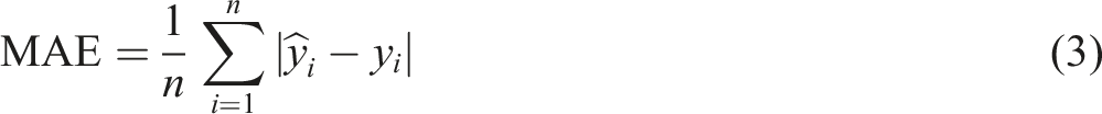
Model performance was evaluated through comparison of the counts-per-hour predicted by the model with the real counts in the pedestrian data. We summarise performance using the mean absolute error (MAE), the mean absolute percentage error (MAPE) and the root mean squared error (RMSE) which are calculated as follows:

MAE = \frac{1}{n} \sum_{i = 1}^{n} | {\hat{y}}_{i} - y_{i} |

(3)

M A P E = \frac{100}{n} \sum_{i = 1}^{n} | \frac{{\hat{y}}_{i} - y_{i}}{y_{i}} |

(4)

R M S E = \sqrt{\frac{\sum_{i = 1}^{n} {({\hat{y}}_{i} - y_{i})}^{2}}{n}}

(5)

where

{\hat{y}}_{i}

is the model prediction for item i, y_i is the real value in the data and n is the total number of data points.

The appropriate buffer size within which to associate built environment data with a sensor (as described in Section 3.2.4) was not intuitive. Daniel and Burns (2018) have pointed to 400m as the distance people are willing to walk before choosing to drive – the so-called ‘pedestrian shed’. However, this does not translate into the distance within which built environment features are influential on the pedestrian dynamics on a street, nor in an area. Indeed it is likely that this distance is inconsistent between different features and different contexts. We therefore chose to base our buffer size on empirical performance, and fitted and evaluated models based upon data sets constructed with a range of buffer sizes (this is discussed in Section 5).

Ultimately a Random Forest Regressor with a buffer size of 400m was selected as the most appropriate model for use in the remainder of this analysis, and is hereafter referred to as the model. Full details of the model comparisons will be provided in Section 5.

Model validation

The ability of the model to generalise to unseen data, and to provide accurate predictions across a spatially diverse urban landscape was then validated. At this stage we opted for a chronological train-test split validation, instead of the K-fold cross-validation used in the model selection process. K-fold is readily applicable and easily understood, and should ensure the model is trained using data from sensors across the city, allowing it to capture the trends in different areas. However, it is liable to produce overly optimistic errors due to data leakage. Data leakage occurs when data from the training set ‘leaks’ into the testing set, thereby giving the model information that it would not usually be able to access and invalidating the assumption of the model being tested on unseen data. This is acceptable in model selection – where each of the models will benefit to the same degree – but for model evaluation a different approach is required.

For final model evaluation, a chronological validation technique was selected. In this approach, the data were ordered chronologically, and then the model was trained on the first 80% of the data and tested on the final 20%. This prevented the possibility of temporal data leakage, which occurs when the model would be able to learn patterns from sensors in the future and apply them whilst making predictions in the past. As sensor deployment was staggered over a long period, a portion of sensors do not begin operating until the final 20% of time. Therefore the chronological split incidentally ensures that the testing set includes sensors that are completely unseen by the model during training, which is necessary to truly assess the generalisability of the model. This validation approach does not attempt to resolve an additional data leakage issue, that of spatial data leakage. This is an open research question and deemed to be outside the scope of this work, and this is discussed further in Section 7.

Feature importance

A secondary objective of this research is to examine how various environmental factors like the weather, infrastructure and others, influence the size of ambient population. ‘Feature importance’ provides insights into the degree to which the various model features affect predictions, indicating their role in modifying the dependent variable. The standard method to determine feature importance in the RandomForestRegressor model from scikit-learn is the ‘impurity-based’ technique, but this can exaggerate the significance of numerical attributes³. Instead, we employ the ‘permutation importance’ method. This approach involves systematically excluding specific features and observing the decrease in the model’s predictive accuracy. Features that do not greatly influence the model’s prediction quality are deemed less crucial.

Results and discussion

Model choice and predictive accuracy

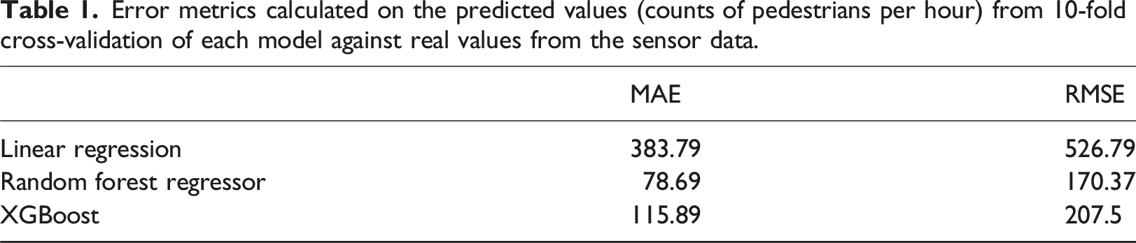
Using standard 10-fold cross validation, the Random Forest Regressor outperformed the linear regression and XGBoost in terms of the MAE and the RMSE in the model selection process (see Table 1). Interestingly buffer sizes from 400 to 1000m had a very limited impact on the difference in errors and so the theoretically-supported (Daniel and Burns, 2018) size of 400m was chosen (see Table 2).

Table 1.

Error metrics calculated on the predicted values (counts of pedestrians per hour) from 10-fold cross-validation of each model against real values from the sensor data.

	MAE	RMSE
Linear regression	383.79	526.79
Random forest regressor	78.69	170.37
XGBoost	115.89	207.5

Table 2.

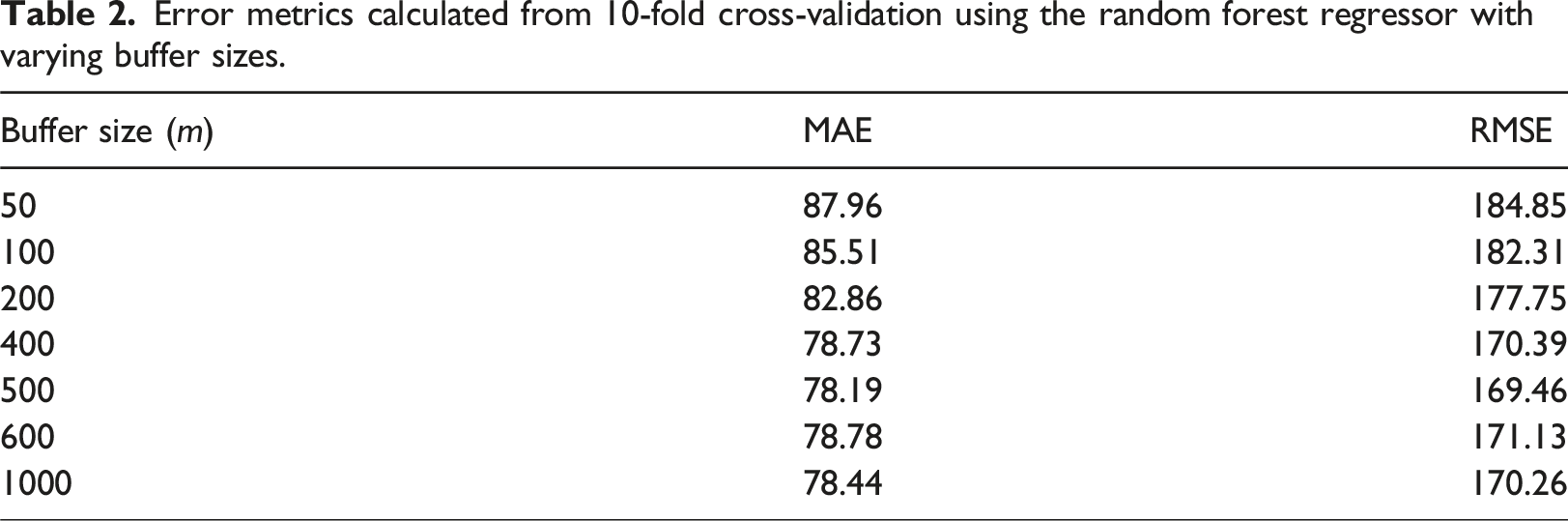
Error metrics calculated from 10-fold cross-validation using the random forest regressor with varying buffer sizes.

Buffer size (m)	MAE	RMSE
50	87.96	184.85
100	85.51	182.31
200	82.86	177.75
400	78.73	170.39
500	78.19	169.46
600	78.78	171.13
1000	78.44	170.26

Having chosen the most appropriate model (the Random Forest Regressor) and a suitable buffer size for the aggregation of spatial features (400m), we now re-train the model using the chronological test-train split method to avoid temporal data leakage (as discussed in Section 4.3). The model was trained on the first 80% of the data and tested on the remaining 20%. Table 3 outlines the associated errors. The errors are slightly larger than those derived using the k-fold cross-validation technique (Table 1) because the chronological validation technique prevents temporal data leakage, ultimately making the prediction task harder.

Table 3.

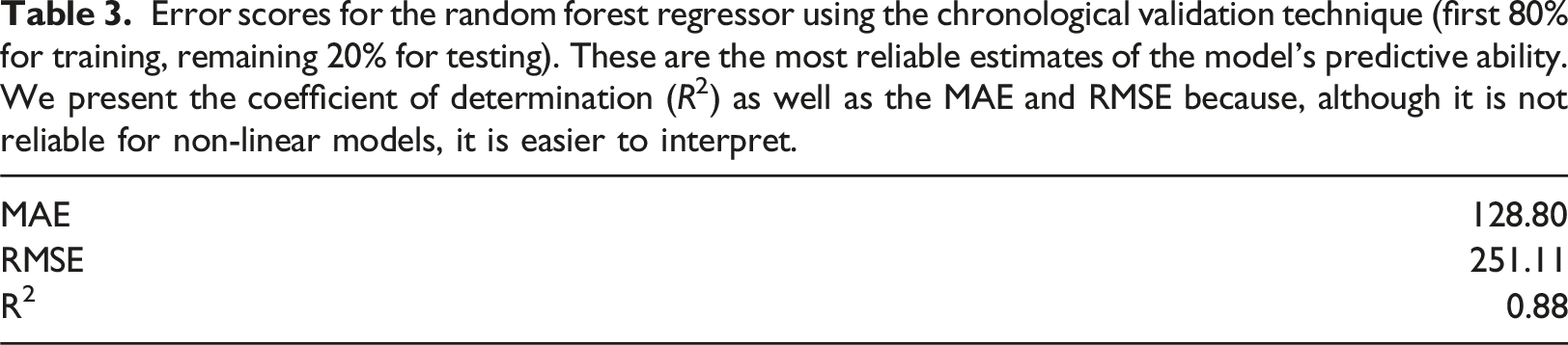
Error scores for the random forest regressor using the chronological validation technique (first 80% for training, remaining 20% for testing). These are the most reliable estimates of the model’s predictive ability. We present the coefficient of determination (R²) as well as the MAE and RMSE because, although it is not reliable for non-linear models, it is easier to interpret.

MAE	128.80
RMSE	251.11
R²	0.88

Plotting the actual values against model predictions illustrates that although there is inherent variability, a majority of the predictions closely align with the diagonal line (x = y) or cluster in close proximity to it (see Figure S4 in the supplemental material). This provides confidence that the model does not exhibit bias toward overestimating or underestimating pedestrian counts.

Temporal accuracy

The prediction error may vary depending on the time-of-day and day-of-week as some time periods may be easier to predict than others. To assess this we observe the mean pedestrian count per hour over 7 days (Monday–Sunday) from the original observation data as well as the mean absolute error (MAE) and mean absolute percentage error (MAPE) as per (3) and (4), respectively. We use the same time period for all sensors (2011-2020). See Figure S5. The MAE varies as expected, showing larger errors during busier times of day. Interestingly, however, the MAPE – that should be relatively stable if the model was able to predict all time periods equally well – is larger in the night-time hours. This suggests that behaviour in these times is harder to predict from the factors provided to the model (weather, built environment, etc.), and implies that perhaps the environment might not be driving pedestrian behaviour during those hours in the way it does at other times.

Spatial/sensor accuracy

We find that the accuracy of model predictions varies spatially as well as temporally, as per Figure S6. As expected, the largest flows are generated by sensors in parts of the city that are likely to be busy (near to the Town Hall, major transport hubs, cultural sites, etc.). However, despite the large flows, these sensors do not produce particularly high absolute (MAE) or percentage (MAPE) errors, suggesting that footfall in these parts of the city is predictable. There are some sensors that are located near places that cause substantial and sporadic increases in footfall, such as the Marvel Stadium, that are much harder for the model predict. This is understandable as it has no information about timings for events at stadiums and other venues.

Feature importance

A benefit with random forest models, over some other machine learning techniques, is that it is possible to extract information about the input parameters (‘features’) that are the most important. Although this does not tell us whether these features are linked with more or less footfall, it does tell us which are the most useful for predicting footfall. To this end, Figure 1 presents the feature importance for the most important features, calculated using the permutation importance metric (see Section 4.4). As the permutation importance itself is difficult to interpret, we also include a random variable in the model (‘random_cat’) that takes integer values between 1 and 3, and only present features whose importance is greater than the importance of this variable. Note the logarithmic scale; the top two variables dominate the importance.

Figure 1.

Feature importance for all variables whose importance is greater than that of a random categorical variable.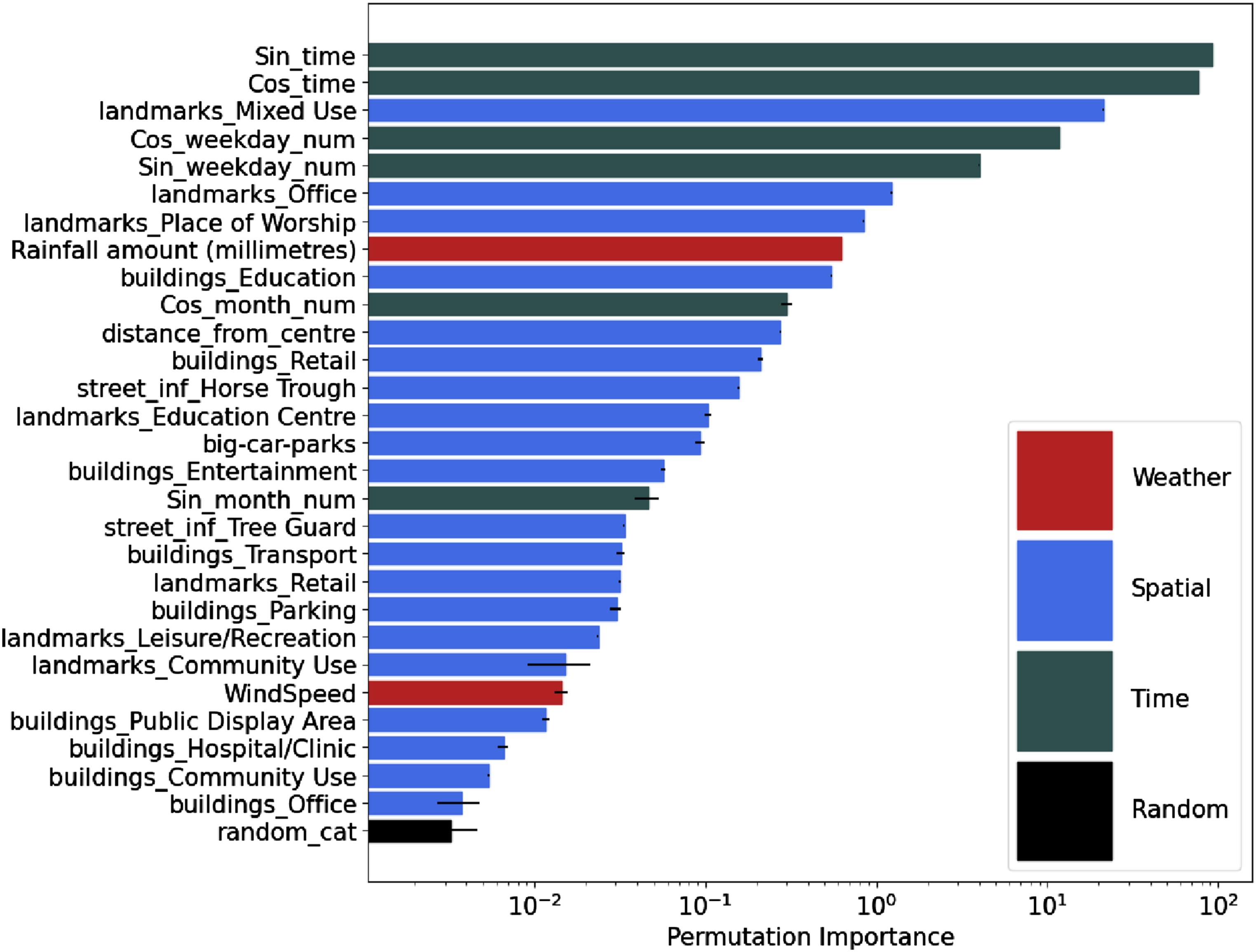

Observing the feature importance, it is not surprising to see time-related variables – ‘Sin_time’, ‘Cos_time’ for time-of-day and ‘Sin_weekday_num’, ‘Cos_weekday_num’ for day-of-week (see Section 3.2.1) – dominating the importance ranking. The time-of-day, in particular, is especially important, as is the day of the week. Rainfall (‘Rainfall amount (millimeters)’) is the most important of the weather variables. Interestingly the temperature (‘Temp’) is not important, but it is possible that this is correlated with rainfall, time-of-day and/or the month, all of which have higher importance. The most important built environment features are ‘landmarks’ which makes sense as these are likely to attract people for leisure, education and commuting. Although some built environment variables, such as horse troughs (‘street_inf_Horse Trough’), are much harder to make sense of, it is likely that these variables are correlated with other features. It is interesting to note that the betweenness of the closest road, which has been previously associated with pedestrian or vehicle traffic (see Section 3.2.4), was not found to be important at all. Similarly the census variables (age, income and education level) were not found to be important. It is possible that if we were to re-run the analysis without the presence of the time variables, or with data aggregated to larger time periods, we may start to identify the differing impacts of different forms of the built environment as the importance may not be swamped by temporal variables. This will be considered for future work.

Evaluating the role of spatial Features

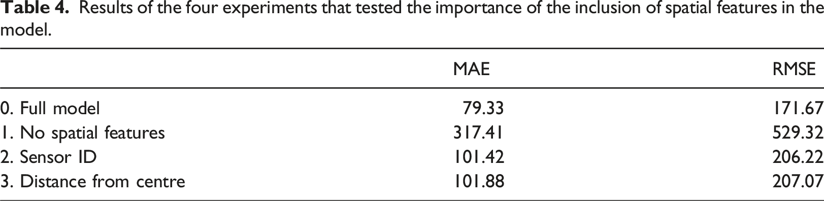
Section 5.3 evidenced spatial variation in the recorded mean footfall count across the sensors – that is, the sensors show that some parts of the city are busier than others. In our research, we aim to explain the underlying factors driving this variation. However, Figure 1 shows that the spatial variables that we included are of limited importance. Perhaps there are alternative spatial variables that are responsible for driving this variation.

To test this, we conducted a series of model experiments, the results of which are presented in Table 4. Initially, we ran the model without the inclusion of any variables describing the spatial environment. Hence there was no way for the model to identify the sensor, and its surroundings, that gave rise to each footfall count. We found that the model’s performance suffered, confirming that spatial patterns do influence the footfall data. In Experiment 2, we introduced the sensor ID as a variable, allowing it to distinguish the origin of the data from different sensors, thus enabling the detection of distinct patterns at each sensor location. While performance improved significantly compared to the first experiment, it remained below that of the full model, indicating that the specific spatial information provided by the variables we included does improve model performance. In the third experiment, we excluded the sensor ID but included a variable representing each sensor’s distance from the central business district. This test assessed whether a simple proximity measure could serve as a proxy for detailed spatial features. The model performed better than in the first experiment and similarly to the second, but still fell short of the full model’s performance. To conclude, these experiments have demonstrated that although the time-related variables are the most important drivers of footfall, the inclusion of variables related to the built environment are also important, and that those we have included here do offer some explanatory power.

Table 4.

Results of the four experiments that tested the importance of the inclusion of spatial features in the model.

	MAE	RMSE
0. Full model	79.33	171.67
1. No spatial features	317.41	529.32
2. Sensor ID	101.42	206.22
3. Distance from centre	101.88	207.07

Evaluation of extraordinary events

One useful application of the model is as a tool to evaluate the extent to which extraordinary events impacted on footfall after taking account of external conditions (day of the week, weather, holiday, the urban environment, etc.). This has a potential value as a policy analysis or urban planning tool as it can allow analysts to gain insight into how an event affected urban dynamics beyond just exploring the raw footfall counts. By allowing the model to estimate footfall during an event and examining the size of the over- (or under-) predictions and the spatio-temporal dynamics of these residuals it would be possible to track any ‘excess’ population, beyond the typical population that would be expected, as it moves around the city. To demonstrate this potential we consider three events: (a) the Anzac Day Parade; (b) New Years Day; and (c) 1 week after the declaration of a COVID-19 state of emergency in Victoria. Figure 2 shows, for each event, how the actual footfall counts on the day varied in comparison to a ‘business as usual’ model prediction for those specific days.

Figure 2.

Event evaluation using the model. Percentage increase between the footfall counts observed by the sensors, compared to those predicted by the model. Left column shows the overall values for each sensor, on each day. Right column shows the overall values for each hour, across all sensors.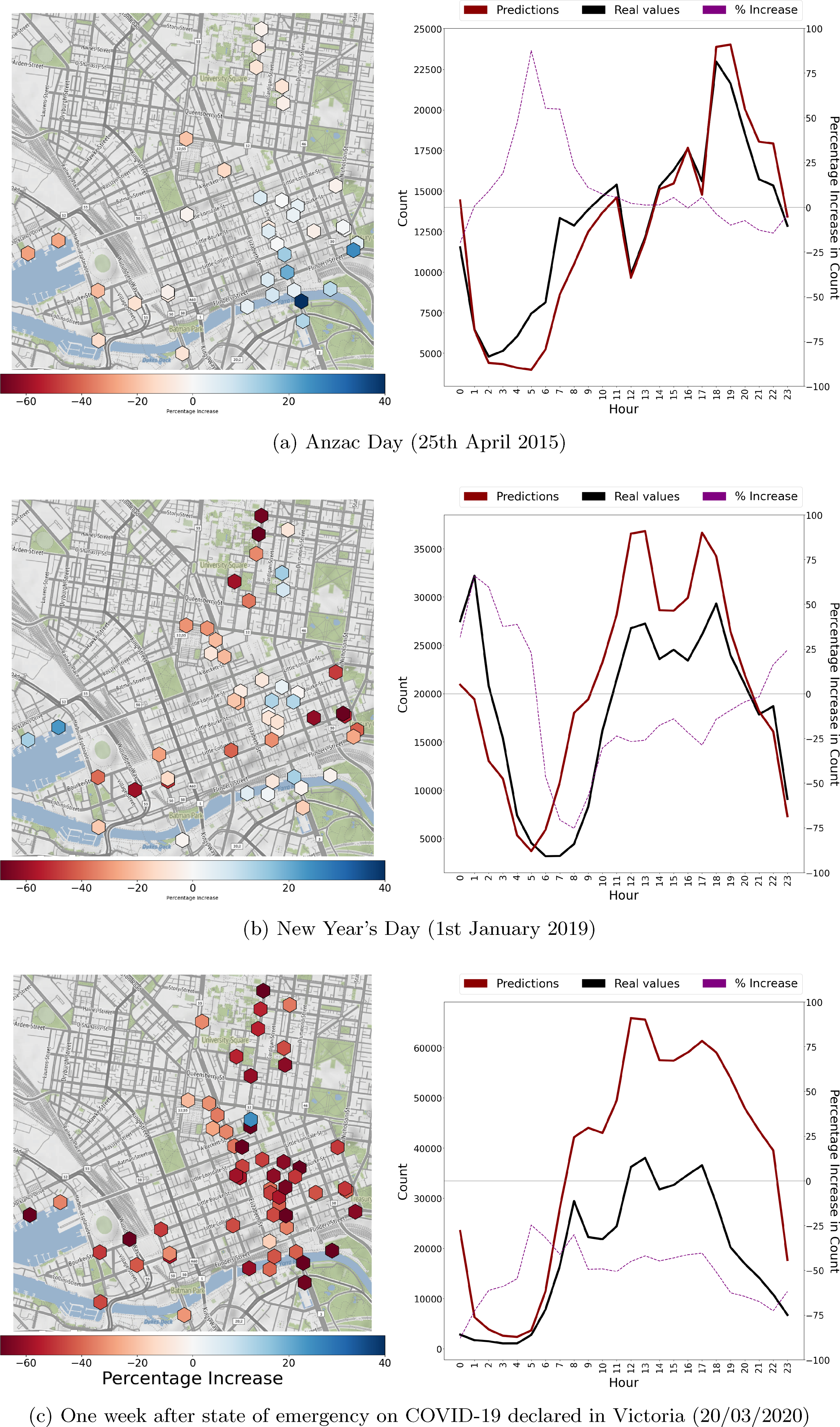

The Anzac Day Parade (Figure 2(a)) is a national day of remembrance that takes place on 25th April every year. We, arbitrarily, study the 2015 parade. On that day, a relatively small mean increase in footfall of 3% was observed across all sensors compared to the model prediction, primarily in the early morning hours. The sensor with the most substantial observed increase in footfall compared to the model prediction was to the south-east of the city, close to the Shrine of Remembrance, where the Anzac Day dawn service is held.

As a second example (Figure 2(b)) we evaluate a New Year’s Day; arbitrarily choosing Tuesday 1st January 2019. Interestingly, there was 12% lower footfall recorded across the whole day than would have been expected from the model prediction for a ‘typical’ Tuesday at the beginning of January. Closer analysis shows that this overall figure hides a 47% increase in footfall between midnight and 3am, and a 22% reduction in footfall between 3am and the subsequent midnight. In the spatial plot, we can also see there are some areas with substantially less footfall than expected, whereas others with substantially more. This shows that the model is revealing insight into the dynamics of new-years day celebrations; both the total numbers of visitors and also, importantly, the high-resolution spatio-temporal fluctuations that would be masked by a more aggregate analysis.

Finally we assess the impact of the onset of the COVID-19 lockdown in Melbourne in 2020. On 16th March the state of Victoria declared COVID to be a public emergency and on 30th March the first official lockdown began. We examine 20th March 2020 to explore citizens’ behaviour in the period after the emergency was declared but before a full lockdown was mandated. Figure 2(c) shows a 50% decrease in foot traffic with considerable spatial variability. Just one sensor, sensor 61, had an increase (of 21%) in footfall compared to projected levels, whilst other areas experienced a relatively modest decline compared to projected levels, while others encountered much more substantial reductions of up to 80%.

Application of the model to Post-COVID data

As discussed in Section 4.1, we choose the time period of the study to avoid the COVID-19 pandemic, restricting the model training, testing and analysis to the full years of 2011–2020. However, in this final piece of analysis, we test the generalisability of the model by applying it to a series of time periods that succeed January 2020. We do this to determine the extent to which the model trained on pre-COVID footfall patterns can be used to predict more recent footfall. This includes predicting new footfall counts on sensors that already exist in the data as well as making predictions on new sensors that have come online since January 2020 and have never been seen before by the model.

Table 5 outlines the time periods chosen and the various errors (MAE, RMSE, R²) that are produced when the model makes predictions on all sensors and all hours available in the given time period. For context, the errors produced by the model that was trained and tested on pre-COVID data (presented previously in Table 3) are MAE = 129, RMSE = 251 and R² = 0.88. The model performs reasonably well when applied to the ‘Pre-COVID’ time period, which is expected as although the footfall patterns in early 2020 might be starting to diverge as awareness of the pandemic becomes more common, they are unlikely to have changed substantially at this point. However, once the pandemic is seen as sufficiently serious by policy makers and lockdowns begin to be introduced, the errors increase substantially to the point that the R² value even becomes negative which suggest that the model prediction is worse than taking the mean footfall (the residual sum of squares exceeds the total sum of squares).

Table 5.

Errors produced by the final model when applied to a selection of pre- and post-COVID time periods. Some model predictions made during the pandemic are so poor that the R² statistic becomes negative. For comparison, the errors produced by the ‘final’ model were MAE = 129, RMSE = 251 and R² = 0.88.

Time period	Start (inclusive)	End (exclusive)	MAE	RMSE	R²
Pre-COVID	2020-01	2020-03	146	281	0.857
During COVID (early 2020)	2020-03	2020-06	415	719	−2.52
During COVID (late 2020)	2020-07	2021-01	477	802	−7.03
During COVID (2021)	2021-01	2022-01	407	722	−2.61
Post-COVID (2022)	2022-01	2023-01	307	585	−0.23
Post-COVID (2023)	2023-01	2024-01	279	540	0.19
Post-COVID (2024)	2024-01	2024-07	294	546	0.0822

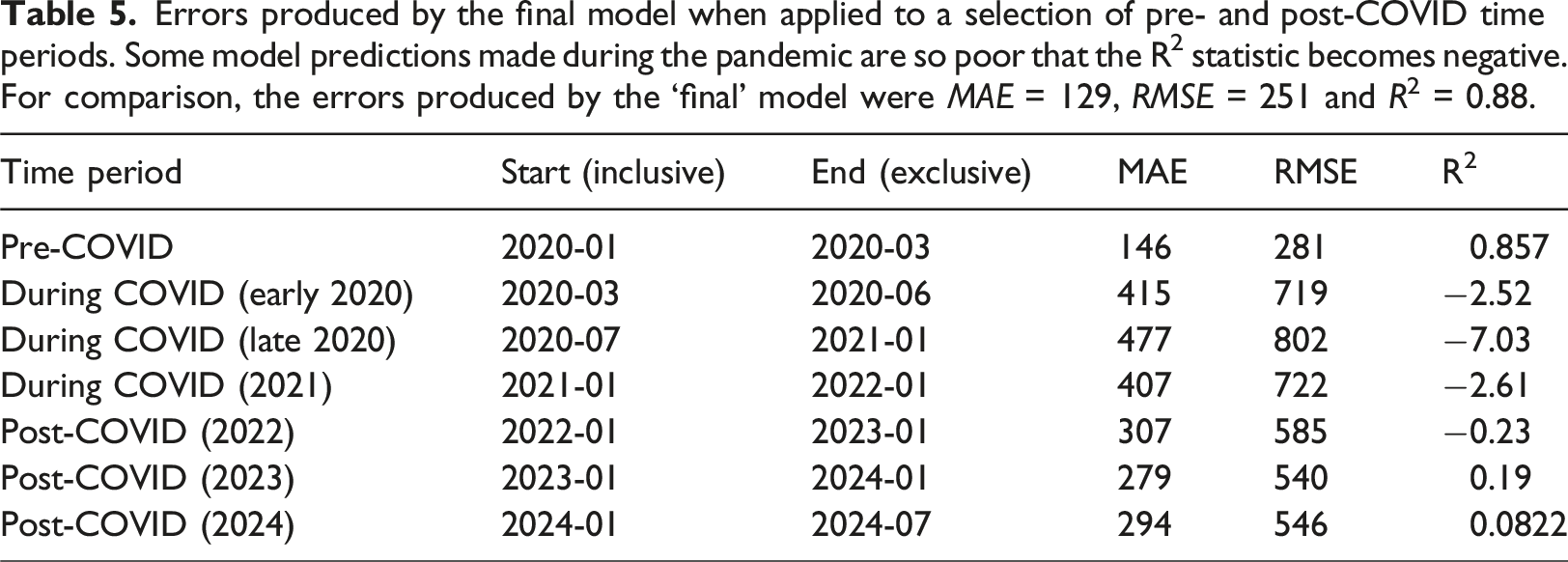
The most interesting finding from Table 5, however, is that the model continues to make poor predictions even when the pandemic begins to subside (the ‘Post-COVID’ time periods). Although the error begins to recover, the model predictions remain much poorer than those produced by testing on the pre-COVID time periods. This could be symbolic of a failure of the model to generalise, but it is equally possible that the footfall patterns in Melbourne have changed substantially after the pandemic and have yet to (or may never) return to their pre-COVID ‘normality’.

Figure 3 provides evidence for this fundamental change in urban dynamics by presenting the total hourly counts aggregated to months for clarity for all sensors across all years. Even though some sensors begin to report very high footfall after 2022 the mean footfall across all sensors (red line) remains substantially lower than the pre-COVID periods.

Figure 3.

The total monthly footfall counts of all sensors (black) and the mean monthly count across all sensors (red). There is a substantial decrease in footfall over the period affected by COVID-19. After that period although some sensors begin to evidence a recovery in footfall counts, the mean remains suppressed.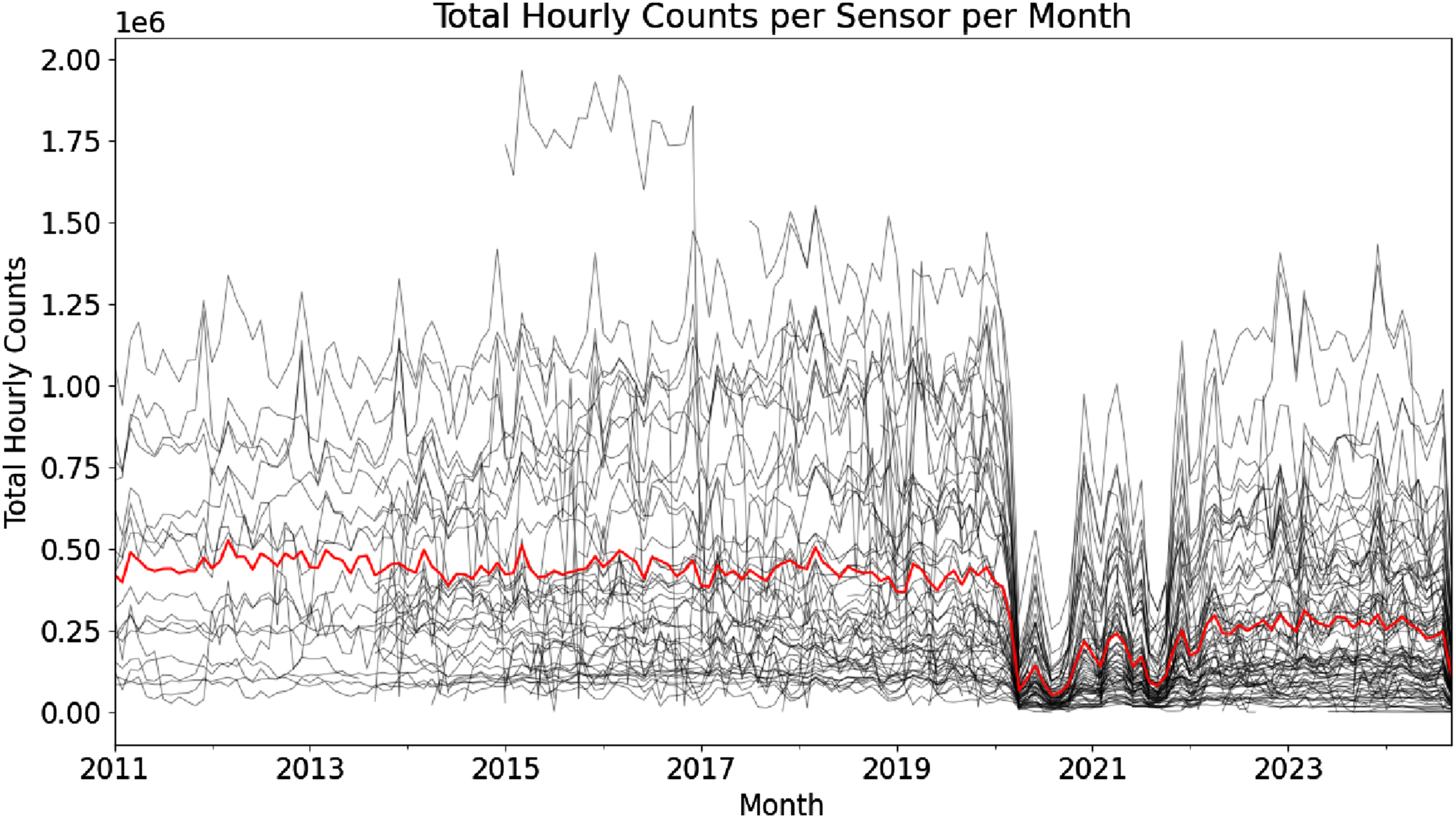

Furthermore, Figure 4 presents the difference between actual values and predicted values for six of the time periods. In the pre-COVID period most predictions sit close to the x = y diagonal, indicating relatively good predictions. For most of the remaining charts, it is clear that the model is making considerable over-predictions, which would be expected if the actual footfall has not recovered post-COVID. In the final chart (‘Post-COVID (2023)’) it appears that some hourly counts have returned to their pre-COVID levels and can be predicted by the model, whereas some still report much lower footfall than would be expected otherwise. This is an important finding as it suggests that in some times and/or places the dynamics of pedestrian footfall may have been permanently disrupted by the pandemic and may not return to their pre-COVID levels. The theoretical and empirical implications of this finding are discussed further in Section 6.

Figure 4.

Plots of the model predictions against actual pedestrian footfall counts for the selection of pre- and post-COVID time periods (the final post-COVID time period is omitted for clarity).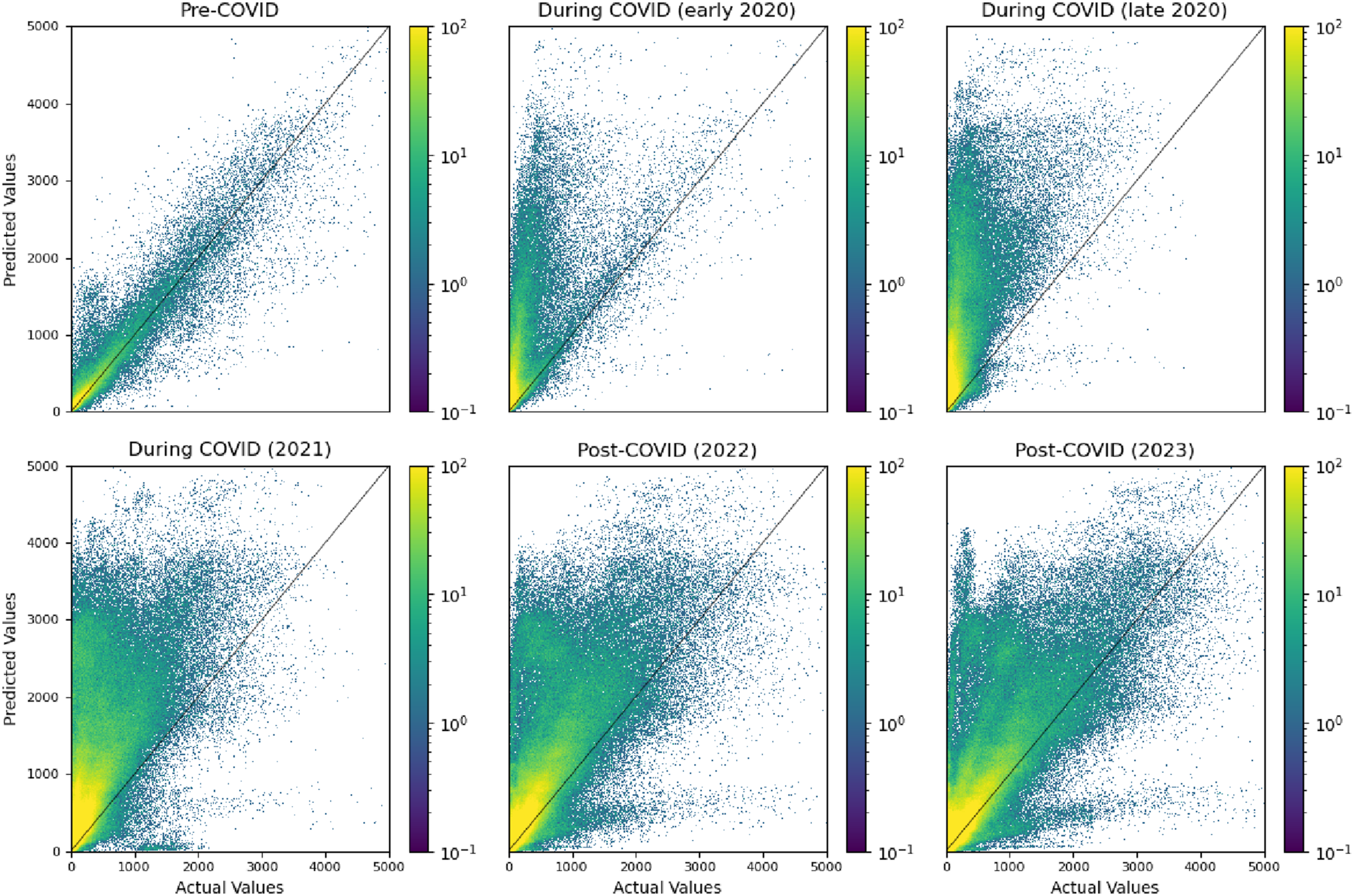

Contribution to geographical and urban theory

By measuring and predicting the ambient population in urban areas using granular spatial variables, our analysis enables the testing of pedestrian movement theories and relates to several established frameworks in urban geography. For example, in the social force model of pedestrian behaviour, next to internal forces between the pedestrians, external and attracting forces ‘act on’ pedestrian flows (Helbing and Molnar, 1995). Certain features of the urban environment might be interpreted as ‘forces’ that have a certain ‘strength’ associated with them. It may also be possible to determine which urban features exert enough force to disrupt the pedestrian flow. In this regard, we found that landmarks associated with work, spiritual worship and mixed uses are significant spatial drivers of the ambient population. Our work thus emphasises that pedestrian movement patterns are not only the result of self-organisation from internal interactions between pedestrians but are also influenced on a larger scale by cultural and economic practices.

This ‘constraint-driven’ view also aligns, for instance, with the concepts of Time Geography (Hägerstrand, 1983). Time Geography is a theory that emphasises the importance of time-space constraints on human movements, suggesting that pedestrian behaviour is influenced by both time availability and the spatial configuration of the city (Hägerstrand, 1983). Our data-driven approach is perhaps particularly interesting in this context for it attempts to make this framework more concrete and quantifiable. For example, Miller (2005) has argued that Time Geography is about n-dimensional ‘constraint-spaces’ that shape human movement and intends to mathematically model these constraints and the emerging human pathways. It is not clear, however, what precisely these constraints are and how to operationalise them. Our approach, which focuses on the drivers of ambient population and movement, can assist in the operationalisation by suggesting which spatio-temporal urban features are relevant to human movement and which ones not so much. Correspondingly, it has previously been suggested that measuring movement is a critical and theory-relevant frontier in geography (Long and Nelson, 2013).

Another quantifiable framework that could considerably benefit from our approach to measuring the ambient population is urban scaling theory. Urban scaling theory makes quantifiable predictions about outcome variables such as economic income, innovation and crime rates, based on a city’s size, including its permanent population and population density (Burger et al., 2022). The development of robust methods to measure the ambient population will be critical in unlocking further study on how the ambient population scales with city size and additionally influences these outcomes.

Finally it is worth noting that we find, in Section 5.7, that the model makes over-predictions of footfall counts even after the end of the pandemic. We provide evidence that this might be caused by a fundamental change in the dynamics of pedestrian activity in Melbourne that the model, trained on pre-COVID footfall patterns, cannot replicate. There is additional evidence for such a shift from other places. For example, Salon et al. (2021) find a ‘stickyness’ to peoples’ behaviour change during the pandemic and suggest a doubling in teleworking and continued increases in online shopping, both of which will have implications for footfall (although it is worth noting that they also predict increases in walking/cycling). Similarly Javadinasr et al. (2022) find ‘significant changes during and after the pandemic in telecommuting, mode choice, online shopping’ and expect most of these impacts to ‘stick’ after the pandemic and shape new dynamics. From a theoretical standpoint, it may be that the pandemic has fundamentally changed the way that many people live and how they choose to engage in their various behaviours.

Limitations and future work

There are several limitations to our approach that might motivate further studies. First, as mentioned in Section 4.3, we do not attempt to avoid the potential for spatial data leakage. This leakage occurs where two sensors are very close to each other and may therefore exhibit similar patterns. If the model is trained on one of those sensors, it will be easy to predict the patterns of its neighbour. There are multiple strategies to mitigate the potential for spatial data leakage, but all risk introducing further problems. For example, we experimented with first partitioning the sensors into distinct spatial clusters using a K-means algorithm and then implementing a cross-validation scheme that ensured sensors in the same cluster were not used in both training and testing. This strategy would be optimal under the condition of a uniform spatial distribution of sensors throughout the urban landscape. However, the actual distribution of sensors is highly uneven. This meant that in any given ‘fold’ of this spatial cross-validation approach, the model was being trained on data from parts of the city that were geographically isolated from the testing locations. Hence the model was being asked to make predictions on neighbourhoods with patterns that it had never been given the chance to understand and incorporate. Of course the model should be able to generalise and make predictions in areas that it has not seen data for, but the standard spatial k-means clustering approach meant that the more residential parts of the city, that have fewer sensors, were all clustered together. Hence the model was asked to learn footfall patterns in more central areas, that have their own distinctive characteristics, and then make predictions on neighbourhoods with entirely different patterns. As the number of sensors increases and more data are collected from less central neighbourhoods then the k-means approach may be more successful as we could create multiple clusters in residential areas so the model would at least be able to learn the general trends in these kinds of neighbourhoods.

We also considered a local segregation approach that was designed to ensure that if two sensors were very close then they would not be separated into distinct testing and training sets. However, this highlighted the problem that some pairs of sensors, although close, measure quite different footfall patterns (one may be focused on a busy highroad and its neighbour may be focused on a quiet adjoining side street). Hence the partitioning scheme should take into account spatial proximity as well as the specific local patterns that the sensor records. Implementing this algorithmically would be an intriguing research question in itself and is beyond the scope of this paper. In conclusion we decided not to try to resolve the problem of spatial data leakage and recommend this as an immediate action for future work.

A second limitation is that while we have employed decision-tree based methods such as random forest regressors, it is plausible to apply other machine learning techniques such as neural networks. Neural networks may outperform our approach when trained on large amounts of data. In future work, data for the city of Melbourne, or other cities, might be re-consolidated and, if sufficient quantities are available, neural networks should be at least compared against our approach.

Third, along with bias that might be introduced through an inequitable spatial distribution of the sensors (that may fail to capture the activities of some socio-demographic groups) there is the more technical problem that some sensors report much more data than others, hence biasing the model to these sensors. However, a straightforward resolution to this issue is elusive, as any apparent solution tends to bring new challenges. An obvious approach to un-biasing would be to use balancing methods such that the volume of data from each sensor was similar. To balance the data, sensors that returned large numbers of counts could be sub-sampled, and those that returned few samples could be over-sampled. However, in the Melbourne data there is a huge disparity in the number of counts returned by the sensors. Hence balancing would either involve considerable over-sampling from the sensors with limited data (which will introduce additional bias) or removing huge amounts of data from the longest-running sensors (which will reduce the accuracy of the model).

Finally, it is important to note that although we include a small number of socio-economic and demographic variables, our analysis largely focuses on impacts of the built environment on footfall. Factors such as deprivation, (perceived) crime levels, etc., will undoubtedly have an impact on whether people choose to walk in an area. The built environment is, after all, only a small part of the overall “environmental backcloth” (Brantingham and Brantingham, 1993). That said, it is not always clear as to whether data on the residential locations of survey participants should be used, or whether ‘ambient population’ data, that capture the attributes of visitors to an area, would better represent the feature of interest. For example, information about the small number of people who may live in a central business district is unlikely to be informative of the activities that characterise such an area, given that many more people will visit it from outside and it is their characteristics that will largely shape the neighbourhood activity patterns.

With respect to future work, an exciting extension of the current study would be to analyse a number of cities from a variety of different countries. Given that publicly available footfall data are already available from a large number of cities – including Bologna, Turin, Dublin, San Diego, Helsinki, among others – and associated data from Open Street Map and weather services are also readily available, such an analysis would be achievable given sufficient resources. It is important to note, however, that even when data are available some considerable effort is required to clean and analyse the footfall data prior to modelling. Unlike official sources, such as population censuses, footfall data are typically uploaded by local authorities that do not always have the resources to routinely detect and fix errors. Even the Melbourne data, that are relatively good quality, required a considerable amount of cleaning and preparation before use.

The paper demonstrated the potential for the model to be used as a policy analysis or planning tool, particularly through the post-hoc investigation into the impacts of extraordinary events on urban dynamics. As local councils and communities adjust to ‘post-COVID’ footfall patterns that, in some circumstances, may not return to their pre-COVID levels, tools that provide evidence for the success of events or activities that are designed to increase footfall are ever more important. By removing outliers and creating a model that predicts footfall under ‘normal’ conditions, the model has the potential to allow policy makers to produce quantitative evidence to evaluate the extent to which their policies have genuinely attracted foot traffic over that which would be expected given other contextual factors. Building on this, another exciting option for further developing this methodology lies in the incorporation of data assimilation techniques. Data assimilation is a process that systematically combines observed data with model predictions to improve the accuracy of the model’s outputs (Kalnay, 2003). In this context, data assimilation could enable continuous updates to the model by integrating real-time observed footfall data from sensors, as has been achieved for agent-based crowd models (Malleson et al., 2020; Wang and Hu, 2015). This would ensure the predictions reflected the evolving pedestrian patterns, and could provide valuable data-driven corrections to the model’s predictions. This integration would not only improve the accuracy of footfall predictions but also enhance their practical applications in urban planning, transportation management, and policy decision-making. Ultimately they could form a key component of a ‘live’ simulation (Swarup and Mortveit, 2020) or a digital twin (Caldarelli et al., 2023; Tao and Qi, 2019).

Conclusions

This paper has presented a machine learning approach for modelling the ‘ambient’ population, measured here using footfall counts generated from on-street sensors. The explanatory variables include features that represent the structure of the built environment, weather conditions and temporal information. We test a linear regression, a boosted decision tree, and a random forest regressor, finding the random forest regressor to outperform the others.

Through feature importance analysis the model demonstrates that time-related variables are substantially more important in explaining the observed variations in footfall patterns than all of the other features. Interestingly, although some built-environment features were found to be important the street betweenness (a measure of how well connected a road is to the wider network) was found not to impact the predictions. The model was also used to evaluate the impact that extraordinary events had on footfall patterns, both spatially and temporally. Using a model such as this could be a valuable tool for policy makers who seek to quantify the success of events that they have organised in their cities. Although there are limitations that future work should attempt to resolve, the paper has demonstrated that the model could be a valuable tool for understanding and modelling footfall, particularly as part of a larger city digital twin.

Supplemental Material

Supplemental Material - Understanding pedestrian dynamics using machine learning with real-time urban sensors

Supplemental Material for Understanding pedestrian dynamics using machine learning with real-time urban sensors by Molly Asher, Yannick Oswald, and Nick Malleson in Environment and Planning B: Urban Analytics and City Science

Footnotes

Acknowledgements

This project has received funding from the European Research Council (ERC) under the European Union’s Horizon 2020 research and innovation programme (grant agreement No. 757455).

Declaration of conflicting interests

The author(s) declared no potential conflicts of interest with respect to the research, authorship, and/or publication of this article.

Funding

The author(s) disclosed receipt of the following financial support for the research, authorship, and/or publication of this article: This work was supported by the European Union’s Horizon 2020 (757455).

ORCID iD

Nick Malleson

Data Availability Statement

The data used in the study are publicly available from the Melbourne Open Data Portal. Instructions and source-code for downloading the data and producing all the results in the paper can be found in the GitHub repository: https://github.com/nickmalleson/footfall/tree/main/MelbourneAnalysis (Malleson, 2025).

Supplemental Material

Supplemental material for this article is available online.

Notes

Molly Asher is a PhD student at the Institute for Climate and Atmospheric Science at the University of Leeds where her research is focused on understanding how future changes to rainfall extremes influence urban flood risk. She holds an MSc in River basin dynamics and management, from the University of Leeds and a BSc in Environmental science from the University of Sheffield. Alongside her PhD she works part-time on research in the School of Geography, at the University of Leeds. This includes work on the DUST project, simulating human systems, using machine-learning and agent-based modelling, and the INTEGRATE project, developing innovate methods to analyse neighbourhood change.

Dr. Yannick Oswald is a Postdoctoral Researcher in Ecological Economics and Computational Social Science at the University of Lausanne, Switzerland. He studies the complex relationships between the environment and the economy, as well as global inequalities in resource use. To this end, he employs a range of simulation methods, including agent-based modelling and input-output modelling.

Dr Nick Malleson is a Professor of Spatial Science and leader of the Institute for Spatial Data Science (ISDS) at the School of Geography, University of Leeds, UK. His research leverages techniques developed in computer science, statistics and machine learning, and applies them to critical social problems that have a strong geographical context. He is best known for my work on agent-based modelling and in the development of machine-learning and geographical information science techniques to solve problems in the domains of criminal justice, mobility and health.

References

Andresen

(2006) Crime measures and the spatial analysis of criminal activity. British Journal of Criminology 46(2): 258–285, ISSN 0007-0955, 1464-3529. DOI: 10.1093/bjc/azi054.

Andresen

(2011) The ambient population and crime analysis. The Professional Geographer 63(2): 193–212. DOI: 10.1080/00330124.2010.547151.

Andresen

Jenion

Reid

(2012) A. An evaluation of ambient population estimates for use in crime analysis. Crime Mapping: Journal of Research Practice 4: 8–31.

Bafna

(2003) Space syntax: a brief introduction to its logic and analytical techniques. Environment and Behavior 35(1): 17–29, ISSN 0013-9165, 1552-390X. DOI: 10.1177/0013916502238863.

Bogomolov

Lepri

Staiano

, et al. (2014) Once upon a crime: towards crime prediction from demographics and mobile data. In: ICMI ’14 Proceedings of the 16th International Conference on Multimodal Interaction. New York, NY, USA: ACM, 427–434. ISBN 978-1-4503-2885-2. DOI: 10.1145/2663204.2663254.

Boivin

Felson

(2017) Crimes by visitors versus crimes by residents: the influence of visitor inflows. Journal of Quantitative Criminology 34: 465–480, ISSN 0748-4518. DOI: 10.1007/s10940-017-9341-1.

Botta

Moat

Preis

(2015) Quantifying crowd size with mobile phone and Twitter data. Royal Society Open Science 2(5): 150162, ISSN 2054-5703. DOI: 10.1098/rsos.150162.

Brantingham

(1993) Nodes, paths and edges: considerations on the complexity of crime and the physical environment. Journal of Environmental Psychology 13(1): 3–28. DOI: 10.1016/S0272-4944(05)80212-9.

Burger

Okie

Hatton

, et al. (2022) Global city densities: Re-examining urban scaling theory. Frontiers in Conservation Science 3: 879934.

10.

Caldarelli

Arcaute

Barthelemy

, et al. (2023) The role of complexity for digital twins of cities. Nature Computational Science 3: 374–381. DOI: 10.1038/s43588-023-00431-4.

11.

Candipan

Phillips

Sampson

, et al. (2021) From residence to movement: the nature of racial segregation in everyday urban mobility. Urban Studies 58(15): 3095–3117, ISSN 0042-0980, 1360-063X. DOI: 10.1177/0042098020978965.

12.

Chen

Sheng

, et al. (2020) Estimating pedestrian volume using Street View images: a large-scale validation test. Computers, Environment and Urban Systems 81: 101481, ISSN 01989715. DOI: 10.1016/j.compenvurbsys.2020.101481.

13.

Chen

, et al. (2022) Examining the association between the built environment and pedestrian volume using street view images. Cities 127: 103734, ISSN 02642751. DOI: 10.1016/j.cities.2022.103734.

14.

City of Melbourne Open Data Portal (2023) Pedestrian historical data.

15.

Cooper

Harvey

Orford

, et al. (2021) Using multiple hybrid spatial design network analysis to predict longitudinal effect of a major city centre redevelopment on pedestrian flows. Transportation 48(2): 643–672.

16.

Crols

Malleson

(2019) Quantifying the ambient population using hourly population footfall data and an agent-based model of daily mobility. GeoInformatica 23: 201–220.

17.

Daniel

Burns

(2018) How steep is that street? Mapping ‘real’pedestrian catchments by adding elevation to street networks. Radical Statistics 121: 26–48.

18.

Enoch

Monsuur

Palaiologou

, et al. (2022) When covid-19 came to town: measuring the impact of the coronavirus pandemic on footfall on six high streets in england. Environment and Planning B: Urban Analytics and City Science 49(3): 1091–1111.

19.

Ewing

Hajrasouliha

Neckerman

, et al. (2016) Streetscape features related to pedestrian activity. Journal of Planning Education and Research 36(1): 5–15.

20.

Felson

Boivin

(2015) Daily crime flows within a city. Crime Science 4(1): 31, ISSN 2193-7680. DOI: 10.1186/s40163-015-0039-0.

21.

Liu

Lan

, et al. (2023) Measuring perceived racial heterogeneity and its impact on crime: an ambient population-based approach. Cities 134: 104188, ISSN 02642751. DOI: 10.1016/j.cities.2022.104188.

22.

Guo

Zhan

, et al. (2020) Coupling mobile phone data with machine learning: how misclassification errors in ambient pm2. 5 exposure estimates are produced? Science of The Total Environment 745: 141034.

23.

Hägerstrand

(1983) In search for the sources of concepts. In: Buttimer

(ed). The practice of geography. Longman, 238–256.

24.

Hanaoka

(2018) New insights on relationships between street crimes and ambient population: use of hourly population data estimated from mobile phone users’ locations. Environment and Planning B: Urban Analytics and City Science 45(2): 295–311, ISSN 2399-8083, 2399-8091. DOI: 10.1177/0265813516672454.

25.

Harvey

Aultman-Hall

Hurley

, et al. (2015) Effects of skeletal streetscape design on perceived safety. Landscape and Urban Planning 142: 18–28.

26.

Helbing

Molnar

(1995) Social force model for pedestrian dynamics. Physical review E 51(5): 4282–4286.

27.

Hipp

Bates

Lichman

, et al. (2019) Using social media to measure temporal ambient population: does it help explain local crime rates? Justice Quarterly 36(4): 718–748, ISSN 0741-8825, 1745-9109. DOI: 10.1080/07418825.2018.1445276.

28.

Javadinasr

Maggasy

Mohammadi

, et al. (2022) The Long-Term effects of COVID-19 on travel behavior in the United States: a panel study on work from home, mode choice, online shopping, and air travel. Transportation Research Part F: Traffic Psychology and Behaviour 90: 466–484, ISSN 13698478. DOI: 10.1016/j.trf.2022.09.019.

29.

Johnson

Andresen

Malleson

(2020) Cell towers and the ambient population: a spatial analysis of disaggregated property crime. European Journal on Criminal Policy and Research 27: 313–333, ISSN 0928-1371. DOI: 10.1007/s10610-020-09446-3.

30.

Kalnay

(2003) Atmospheric Modeling, Data Assimilation and Predictability. Cambridge: Cambridge University Press.

31.

Leccese

Lista

Salvadori

, et al. (2020) On the applicability of the space syntax methodology for the determination of street lighting classes. Energies 13(6): 1476, ISSN 1996-1073. DOI: 10.3390/en13061476.

32.

Lee

Koschinsky

Talen

(2018) Planning tools for walkable neighborhoods: zoning, land use, and urban form. Journal of Architectural and Planning Research 35(1): 69–88, ISSN 07380895. URL. https://www.jstor.org/stable/45215820

33.

Liu

Lan

Eck

, et al. (2022) Assessing the intraday variation of the spillover effect of tweets-derived ambient population on crime. Social Science Computer Review 40(2): 512–533, ISSN 0894-4393, 1552-8286. DOI: 10.1177/0894439320983825.

34.

Long

Nelson

(2013) A review of quantitative methods for movement data. International Journal of Geographical Information Science 27(2): 292–318.

35.

Malleson

(2025) Data available at Melbourne Open Data Portal. Environment and Planning B: Urban Analytics and City Science. Available at: https://github.com/nickmalleson/footfall/tree/main/MelbourneAnalysis.

36.

Malleson

Andresen

(2015a) The impact of using social media data in crime rate calculations: shifting hot spots and changing spatial patterns. Cartography and Geographic Information Science 42(2): 112–121, ISSN 1523-0406, 1545-0465. DOI: 10.1080/15230406.2014.905756.

37.

Malleson

Andresen

(2015b) Spatio-temporal crime hotspots and the ambient population. Crime Science 4(1): 10, ISSN 2193-7680. DOI: 10.1186/s40163-015-0023-8.

38.

Malleson

Andresen

(2016) Exploring the impact of ambient population measures on London crime hotspots. Journal of Criminal Justice 46: 52–63, ISSN 00472352. DOI: 10.1016/j.jcrimjus.2016.03.002.

39.

Malleson

Minors

Kieu

L-M

, et al. (2020) Simulating crowds in real time with agent-based modelling and a particle filter. The Journal of Artificial Societies and Social Simulation 23(3): 3, ISSN 1460-7425. DOI: 10.18564/jasss.4266.

40.

Martin

Cockings

Leung

(2015) Developing a flexible framework for spatiotemporal population modeling. Annals of the Association of American Geographers 105(4): 754–772, ISSN 0004-5608. DOI: 10.1080/00045608.2015.1022089.

41.

Miller

(2005) A measurement theory for time geography. Geographical Analysis 37(1): 17–45.

42.

Moudon

(2009) Real noise from the urban environment: how ambient community noise affects health and what can be done about it. American Journal of Preventive Medicine 37(2): 167–171.

43.

Njilla

Pearlstein

X-W

, et al. (2019) Internet of things anomaly detection using machine learning. In: 2019 IEEE Applied Imagery Pattern Recognition Workshop (AIPR). Piscataway: IEEE, 1–6.

44.

Panczak

Charles-Edwards

Corcoran

(2020) Estimating temporary populations: a systematic review of the empirical literature. Palgrave Communications 6(1): 87, ISSN 2055-1045. DOI: 10.1057/s41599-020-0455-y.

45.

Park

Kwan

M-P

(2017) Individual exposure estimates may be erroneous when spatiotemporal variability of air pollution and human mobility are ignored. Health and Place 43: 85–94, ISSN 13538292. DOI: 10.1016/j.healthplace.2016.10.002.

46.

Picornell

Ruiz

Borge

, et al. (2019) Population dynamics based on mobile phone data to improve air pollution exposure assessments. Journal of Exposure Science and Environmental Epidemiology 29(2): 278–291.

47.

Pucher

Renne

(2003) Socioeconomics of urban travel: evidence from the 2001 NHTS. Transportation Quarterly 52: 49–77.

48.

Runa

Singleton

(2021) Assessing the impacts of weather on pedestrian signal activity at 49 signalized intersections in northern Utah. Transportation Research Record 2675(6): 406–419.

49.

Salon

Conway

Capasso Da Silva

, et al. (2021) The potential stickiness of pandemic-induced behavior changes in the United States. Proceedings of the National Academy of Sciences 118(27): e2106499118, ISSN 0027-8424, 1091-6490. DOI: 10.1073/pnas.2106499118.

50.

Song

Cai

Liu

, et al. (2023) Effects of ambient population with different income levels on the spatio-temporal pattern of theft: a study based on mobile phone big data. Cities 137: 104331, ISSN 02642751. DOI: 10.1016/j.cities.2023.104331.

51.

Stefanidis

Crooks

Radzikowski

(2013) Harvesting ambient geospatial information from social media feeds. Geojournal 78(2): 319–338. DOI: 10.1007/s10708-011-9438-2.

52.

Swarup

Mortveit

(2020) Live simulations. In Proceedings of the 19th International Conference on Autonomous Agents and MultiAgent Systems. Gaza: AAMAS ’20, 1721–1725.

53.

Tao

(2019) Make more digital twins. Nature 573(7775): 490–491, ISSN 0028-0836, 1476-4687. DOI: 10.1038/d41586-019-02849-1.

54.

Thakur

Bhaduri

Piburn

, et al. (2015) PlanetSense: a real-time streaming and spatio-temporal analytics platform for gathering geo-spatial intelligence from open source data. In Proceedings of the 23rd SIGSPATIAL International Conference on Advances in Geographic Information Systems. Seattle Washington: ACM, 1–4. ISBN 978-1-4503-3967-4. DOI: 10.1145/2820783.2820882.

55.

Trasberg

Soundararaj

Cheshire

(2021) Using wi-fi probe requests from mobile phones to quantify the impact of pedestrian flows on retail turnover. Computers, Environment and Urban Systems 87: 101601.

56.

Traunmueller

Quattrone

Capra

(2014) Mining mobile phone data to investigate urban crime theories at scale. In Aiello

McFarland

(ed) Social Informatics. Cham: Springer International Publishing, 8851, 396–411. ISBN 978-3-319-13733-9 978-3-319-13734-6. DOI: 10.1007/978-3-319-13734-6_29.

57.

United Nations, Department of Economic and Social Affairs, Population Division (2018) World Urbanization Prospects: The 2018 Revision (ST/ESA/SER.A/420). New York: United Nations.

58.

Wang

(2015) Data assimilation in agent based simulation of smart environments using particle filters. Simulation Modelling Practice and Theory 56: 36–54, ISSN 1569-190X. DOI: 10.1016/j.simpat.2015.05.001.

59.

Whipp

Malleson

Ward

, et al. (2021a) Towards a comprehensive measure of the ambient population: building estimates using geographically weighted regression. Preprint, SocArXiv.

60.

Whipp

Malleson

Ward

, et al. (2021b) Estimates of the ambient population: assessing the utility of conventional and novel data sources. ISPRS International Journal of Geo-Information 10(3): 131, ISSN 2220-9964. DOI: 10.3390/ijgi10030131.

61.

Zheng

Chen

, et al. (2023) Exploring the influence of individual daily activity patterns on activity-space segregation. Transactions in Urban Data, Science, and Technology 2(1): 19–38, ISSN 2754-1231, 2754-1231. DOI: 10.1177/27541231231151223.

Supplementary Material

Please find the following supplemental material available below.

For Open Access articles published under a Creative Commons License, all supplemental material carries the same license as the article it is associated with.

For non-Open Access articles published, all supplemental material carries a non-exclusive license, and permission requests for re-use of supplemental material or any part of supplemental material shall be sent directly to the copyright owner as specified in the copyright notice associated with the article.

0.00 MB

0.46 MB