Sage Journals: Discover world-class research

Abstract

Planning and development decisions in both the government and business sectors often require small area population forecasts. Unfortunately, current methods often produce forecasts that are inaccurate, particularly for remote areas and those with smaller populations. Such inaccuracy necessitates the development and evaluation of methods to forecast and communicate forecast uncertainty, however, little research has been conducted in this domain for small area populations. In this paper, we evaluate a set of probabilistic forecasting methods which include Autoregressive integrated moving average, Exponential Smoothing, THETA, LightGBM and XGBOOST, to produce point forecasts and 80% prediction intervals for Australian SA2 small area populations. We also investigate methods to combine the intervals to produce ensemble forecasts. Our results show that individual probabilistic methods generally produce prediction intervals which underestimate forecast uncertainty. Combining forecasts improves the overall accuracy of point forecasts and the coverage of their intervals, however, coverage still tends to be less than the expected 80% for all but the most conservative combination method.

Keywords

Uncertainty urban analytics urban planning demographic change growth and change analysis

Introduction

One of the key elements of urban planning is the forecasting of local area populations. Such small area population forecasts are used widely by both governments and businesses to guide planning and development decisions. Current practices often produce forecasts which are inaccurate, particularly for areas which are remote and have small populations (Wilson and Rowe, 2011). Methods applied are generally deterministic, producing point forecasts which give users no indication of uncertainty. However, planning decisions would benefit from an understanding of the uncertainty of the predictions that are being used (Keilman, 2020). A recent review of the small area population forecasting literature found that very few projection methods incorporate any indications of forecast uncertainty (Wilson et al., 2021a). As pointed out by Keyfitz (1981), whilst demographers cannot be held responsible for providing inaccurate forecasts, they are responsible for ‘…warning one another and our public what the error of our estimates is likely to be’ (Keyfitz, 1981, p. 579). Therefore, given the extensive use of small area forecasts it is vital that methods to calculate and communicate forecast uncertainty be developed and evaluated.

Statistical agencies often communicate forecast uncertainty by applying a scenario-based approach and creating low, medium and high variants of deterministic forecasts. However, such an approach doesn’t explicitly provide uncertainty measures and it does not enable forecast users to ascertain the likelihood that a future population will fall within a certain range (Tayman, 2011). Furthermore, forecast users often give little attention to the high and low variants and focus on the medium forecast (De Beer, 1997). A more useful method is to create forecasts with prediction intervals which give a predicted range into which a future value is expected to fall, provide a better representation of uncertainty and encourage forecast users to consider a range of population outcomes in their decision-making.

Prediction intervals can be generated using probabilistic forecasting methods, empirical investigations of past forecast errors, or a combination of the two (Rayer et al., 2009). Whilst deterministic methods remain the norm, probabilistic methods are now commonly applied to generate forecasts for countries (e.g. Azose et al., 2016; Keilman et al., 2002; Okita et al., 2011; United Nations, 2019; Wilson and Bell, 2004) and large sub-national geographic areas (e.g. Setiawan et al., 2021; Tayman et al., 2007; Wilson and Bell, 2007). As we move to smaller areas such as local council areas or census tracts, probabilistic forecasts become ‘more challenging’ (Statistics New Zealand, 2016, p. 78).

Quantitative, out-of-sample evaluations of the accuracy of prediction intervals for small areas are rare and challenging. Rayer et al. (2009) generated empirical prediction intervals for US counties by examining the forecast errors produced by extrapolative models. They found that 90^th percentile errors for trimmed mean forecasts of the prior period provided reasonably good estimates of 90% prediction intervals for the subsequent period. Wilson et al. (2018) generated empirical prediction intervals for Australian local area population forecasts based on past error distributions. Simpson et al. (2020) similarly created empirical prediction intervals for English local authority areas by using errors of past cohort-component forecasts for prior years and applying them to later periods. A few papers have also developed and evaluated model-based prediction intervals. Zhang and Bryant (2020) developed a Bayesian approach to estimating and forecasting internal migration for Iceland. Bryant and Graham (2013) used a Bayesian approach to estimate and forecast the components of population change, whilst Jiang et al. (2007) used an approach based on the Hidden Markov model to create point forecasts and prediction intervals for suburbs of Canberra, Australia. The literature on the application of machine learning algorithms for the probabilistic forecasting of small area populations is scarce even though such methods have previously been shown to be the most accurate approaches for creating prediction intervals in the M4 (Makridakis et al., 2018) and M5 (Makridakis and Spiliotis, 2021) forecasting competitions. These M series forecast competitions challenge forecasters to create the most accurate forecasting methods and evaluate them on a large dataset of time series (Makridakis et al., 2020).

The purpose of this research is to provide a comprehensive evaluation of probabilistic forecasting methods. We consider statistical and machine learning models, and combinations thereof, for Australian SA2 areas (Australian Bureau of Statistics, 2017a); these areas are the smallest units in the Australian Bureau of Statistics geographical hierarchy for which population statistics are regularly collected and published. This work will advance prior research by Grossman et al. (2022) which investigated combination methods for Australian SA2s but focused exclusively on deterministic forecasts and included a slightly different set of individual models. Specifically, this paper has the following objectives:

1. To identify probabilistic models that produce the most accurate forecasts with the best coverage.

2. To investigate methods to combine the interval forecasts produced by our set of probabilistic models.

3. To investigate how the results are influenced by the remoteness of the SA2 areas.

In this study, we generate population forecasts with 5 and 10 years forecast horizons for Australian small areas. The “Results” section presents the model evaluation results which are then discussed in the “Discussion” section. The aims, findings, and implications are then summarised in the “Conclusions” section.

Data and methods

Data

We prepared and evaluated probabilistic forecasts with 80% prediction intervals using the 2016 mid-year Estimated Resident population (ERP) totals for Australian SA2 areas (Australian Bureau of Statistics, 2017a). ERPs are produced by the Australian Bureau of Statistics using the place of usual residence data collected during the 5 yearly census. Data on births, deaths and migrations and administrative data are used to adjust sub-state ERPs during census years and estimate populations between census years. ERPs are revised after the subsequent census (Queensland Government Statistician’s Office, 2019). The estimates are generally good quality according to the post-enumeration survey findings, which found that for SA2s with total populations greater than 1,000, the average 2016 absolute intercensal difference was 3.5% (Australian Bureau of Statistics, 2017b).

The 2016 dataset includes population totals from 1991 to 2016, and the median across areas in 2016 was 9681. Two sets of forecasts were prepared for two different jump-off years: 10- years forecasts from 2006, and 5 years forecasts from 2011. These forecasts covered the 2066 SA2 areas whose populations remained above 100 for the duration of the base period.

Methods

In our study, we use three statistical models and two machine learning models to generate point and probabilistic forecasts. Here, the probabilistic forecasts are provided to demonstrate the uncertainty of the model forecasts, where it is expressed in the form of a probability distribution. Specifically, we provided the point forecast and 80% prediction intervals for each attested model. We implemented the three statistical models (ARIMA, ETS and THETA) using the ‘forecast’ package (Hyndman and Khandakar, 2008; Hyndman et al., 2022) in the R programming language, whereas gradient boosting based machine learning models (LGBM and XGBOOST) were developed using the packages ‘lighgbm’ (Ke et al., 2021) and ‘sklearn’ (Pedregosa et al., 2011) in Python.

We generate the prediction intervals for statistical models, assuming the residuals produced from these models are uncorrelated and normally distributed. This assumption is valid because the statistical models, that is, ETS, ARIMA and THETA are capable of capturing time series seasonalities and trends, that is, mostly the trend patterns observed in population-based datasets. In contrast to statistical models, machine learning based models produce prediction intervals based on quantile loss, independent of model residuals being uncorrelated.

The ‘forecast’ package generates the probabilistic forecasts assuming the prediction intervals are wider as the forecast horizon increases. Based on the standard deviation of the forecast distribution, the ‘forecast’ package computes the probabilistic forecasts relevant for a specific prediction interval. We use the level parameter, in the ‘forecast’ package to generate probabilistic forecasts relevant for the 80% of prediction interval. To produce probabilistic forecasts with machine learning models, we use quantile loss functions that attempt to optimise the model for a specific forecast quantile.

Autoregressive integrated moving average (ARIMA)

The Autoregressive integrated moving average (ARIMA) model is widely used for time series forecasting (Box et al., 2015). ARIMA models aim to describe autocorrelations in the time series data. An ARIMA model is a composition of differencing with autoregression (AR) and moving average (MA) components. Here, the AR component uses the lagged values of a time series in a regression model, whereas the MA component uses past forecast errors (residual errors) in a regression model. The integration (I) term represents the degree of differencing (d) applied for the time series to become stationary. A general class of an ARIMA(p,q,d) model can be defined as

X_{t} = c + \sum_{i = 1}^{p} ϕ_{i} X_{t - i} + \sum_{j = 1}^{q} θ_{j} ε_{t - j} + ε_{t}

(1)

In equation (1), X_t is the time series, p denotes the order of lags in the AR model and q denotes the order of error terms in the MA model. Moreover, c is a constant, ε_t is a white noise error term and ϕ and θ are the model parameters. We used the auto.arima function from the R package ‘forecast’ (Hyndman and Khandakar, 2008; Hyndman et al., 2022). This implementation uses the corrected Akaike’s Information Criterion (AIC_c) to determine the optimal order of an ARIMA model, that is, p, q, while the Kwiatkowski–Phillips–Schmidt–Shin test is used to identify the required d to make the time series stationary.

Exponential smoothing (ETS)

The Exponential Smoothing (ETS) algorithm generates forecasts from a weighted average of past observations, with the weights of the past observations set to decrease exponentially as the observations get older. A simple ETS model can be defined as

{\hat{X}}_{t + 1 | t} = α X_{t} + α (1 - α) X_{t - 1} + α {(1 - α)}^{2} X_{t - 2} + \dots

(2)

In equations (2) and (0) ≤ α ≤ 1 refers to the smoothing parameter that controls the influence of the past observations in the time series X₁,. . . , X_t towards X_t+1, which is the one-step-ahead forecast for X_t. In this way, α assigns higher weights to more recent observations, whereas smaller weights are assigned to older observations. In our experiments, we used the ets function from the ‘forecast’ package (Hyndman and Khandakar, 2008; Hyndman et al., 2022). The AIC_c information criterion is used to determine the optimal ETS model for a given time series.

THETA

THETA is a relatively simple statistical model used widely by forecasting practitioners which extrapolates the trend and the level of a series (Assimakopoulos and Nikolopoulos, 2000). The THETA model firstly decomposes a time series into a new set of series, known as Theta-lines, and afterwards applies a forecasting method to extrapolate the Theta-lines separately. Here, exponential smoothing methods are often used as the forecasting method to extrapolate the Theta-lines. The THETA model is also treated as a special case of the simple exponential smoothing with drift (SES) method (Hyndman and Billah, 2003). The final forecasts of the time series are obtained by combining the individual forecasts of Theta-lines. Compared to ETS, the THETA model is incapable of modelling seasonal patterns. However, it can capture time series trends and often deal with short time series better compared to seasonal models such as ETS and ARIMA.

The THETA model performed well for the forecasting of yearly time series in the M3 competition (Makridakis and Hibon, 2000), and it was also included as a base model in the feature-based forecast combination (FFORMA) framework that achieved the second-best results in the M4 competition (Makridakis et al., 2018). As small area populations datasets often deal with yearly, non-seasonal time series data, we have included the THETA model in our evaluation of probabilistic forecasting models for small area populations. We used the THETAf function from the package ‘forecast’ (Hyndman and Khandakar, 2008; Hyndman et al., 2022) to obtain the THETA forecasts for a given population time series.

Gradient boosting models (GBM)

Gradient Boosting Models (GBM) are a popular class of machine learning algorithms based on decision trees that can be used to solve a wide range of machine learning problems. The fundamental idea of GBMs is to use an ensemble of weak decision-tree learners sequentially, where each weak learner attempts to improve on the error from the previous model. As this process is repeated sequentially, GBMs are also referred to as sequential ensemble decision-tree models. In the machine learning literature, Extreme Gradient Boosting (XGBoost) models (Chen and Guestrin, 2016) and Light Gradient Boosting (LGBM) models (Ke et al., 2017) are identified as the most popular variants of GBMs, due to their promising model accuracy and computational efficiency. The main structural difference between XGBoost and LGBM is that XGBoost uses a depth-wise algorithm to grow the decision-tree, while LGBM employs a leaf-wise algorithm.

The competitive performance of LGBMs has been recently demonstrated in the M5 Forecasting Competition, where a globally trained LGBM-based solution achieved first place in both point and uncertainty prediction tracks, followed by many other LGBM-based solutions headlining the rankings (Makridakis et al., 2022). In our study, we use both XGBoost and LGBM architectures to generate point and probabilistic forecasts for small area populations.

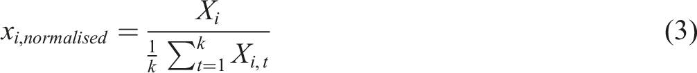
Total populations vary considerably between different SA2s, that is, some areas have populations in the 100s, and others in the 10,000s. Machine learning models which are trained globally across time series often require the time series within a dataset to be on the same scale for optimal performance. Thus, we first pre-processed the time series in our dataset using the recommendations of Bandara et al. (2020) and Hewamalage et al. (2021), and applied the meanscale transformation strategy, where each time series was divided by its mean value using the equation below

x_{i, n o r m a l i s e d} = \frac{X_{i}}{\frac{1}{k} \sum_{t = 1}^{k} X_{i, t}}

(3)

where X_i,normalised represents the ith normalised population time series, and k is the number of observations in time series X_i, where i ∈ {1, 2, · · ·, n}. Here n refers to the total number of time series in the dataset.

After normalising each time series, we applied the Moving Window (MW) transformation strategy to convert time series observations into input and output frames following the recommendations of (Hewamalage et al., 2021). The generated input and output frames were then pooled together and trained as a global model. Figure 1 shows an example of a single input and output window. Here, we assumed the size of the input window sequence {x₁, x₂, ..., x_N} is N and the size of the output window sequence {y₁, y₂, ..., y_M} is equivalent to M. Following the Multi-Input Multi Output (MIMO) strategy in multi-step forecasting (Hewamalage et al., 2021), we made the size of the output window M identical to the intended forecasting horizon. The MIMO is a direct forecasting strategy widely used in the forecast literature (Ben Taieb et al., 2012) that enables direct forecasts of all future values up to the intended forecasting horizon. As the default implementation of XGBoost and LGBM models are only able to train single output from a given set of inputs, we trained models separately for each forecast horizon. In other words, we train M number of models to generate forecasts for the intended forecast horizons. In our experiments, we set the value of M to 5 and 10 to generate 5-years and 10-years ahead probabilistic forecasts, respectively. As exogenous variables, we used the mean and the standard deviation of each input frame to train the XGBoost and LGBM models.

Figure 1.

The input and output window training procedure.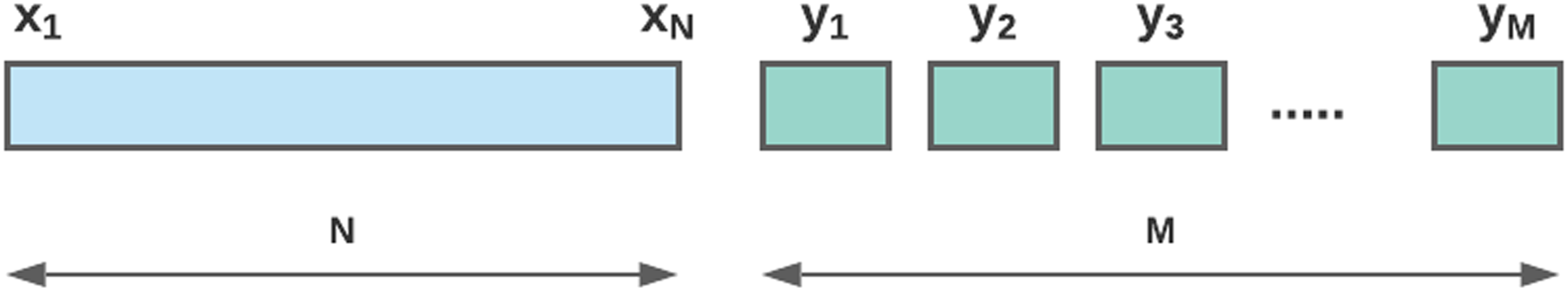

As discussed in Januschowski et al. (2021), GBMs can be trained with any loss function. Therefore, we use the quantile loss function to train the XGBoost and LGBM models to generate probabilistic forecasts for the required prediction intervals. Given a forecast ${\hat{y}}_{t}$ and actual observation y_t, the quantile loss L_t for a given quantile τ at time t is defined as follows

L_{t} = {\begin{array}{c} (y_{t} - {\hat{y}}_{t}) τ, (y_{t} \geq {\hat{y}}_{t}) \\ ({{\hat{y}}_{t} - y}_{t}) (1 - τ), ({\hat{y}}_{t} > y_{t}) \end{array}

(4)

In equation (4), as the τ value lies within 0–1 range, the first term becomes positive when y_t ≥

{\hat{y}}_{t}

, representing the under-forecasting scenario, whereas second term becomes positive when

{\hat{y}}_{t}

> y_t, representing the over-forecasting scenario. When τ is set to 0.5, under-forecasting and over-forecasting are penalised by the same factor, representing the median forecasts. In our study, to obtain the 80% prediction interval, we use the τ values of 0.90 and 0.10, which generated the required upper-level and lower-level forecasts.

To implement the LGBM model, we use the lightgbm function from the Python package ‘lightgbm’ (Ke et al., 2021), whereas the GradientBoostingRegressor function from the Python package ‘sklearn’ (Pedregosa et al., 2011) is used to run the XGBoost models.

XGBoost and LGBM models contain numerous hyper-parameters, which need to be optimised for a given dataset. To achieve this, we created a validation dataset from the pre-processed training data, that is, input and output window tuples, so the model hyper-parameters can be optimised on this unseen portion of the training data. We used 80%, 20% splitting criteria to divide the original pool of windows to training and validation data. We used an autonomous hyper-parameter optimisation framework, Hyperopt (Bergstra et al., 2013), a python implementation of a Bayesian hyper-parameter optimisation process to identify the optimal values for these hyper-parameters. Table 1 and Table 2 summarise the ranges of hyper-parameter values explored for the LGBM and XGBoost models.

Table 1.

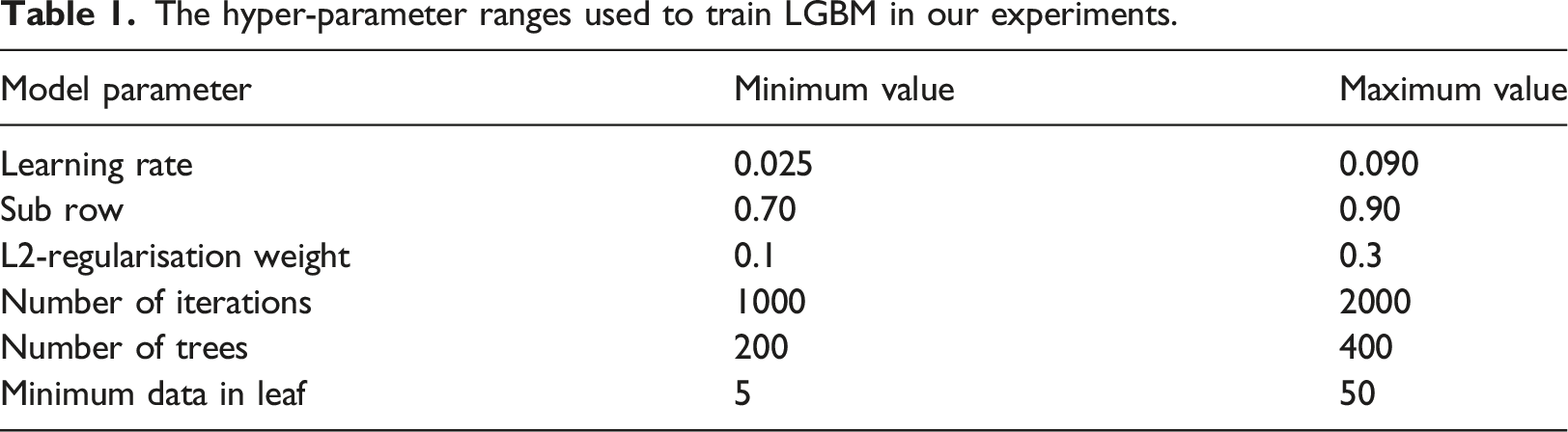
The hyper-parameter ranges used to train LGBM in our experiments.

Model parameter	Minimum value	Maximum value
Learning rate	0.025	0.090
Sub row	0.70	0.90
L2-regularisation weight	0.1	0.3
Number of iterations	1000	2000
Number of trees	200	400
Minimum data in leaf	5	50

Table 2.

The hyper-parameter ranges used to train XGBoost in our experiments.

Model parameter	Minimum value	Maximum value
Learning rate	0.1	0.90
Subsample	0.7	0.90
N estimators	1000	2000
Max depth	2	10
Minimum samples in leaf	5	50

Ensemble models

Combining forecasts often produces improved accuracy due to a reduction in model variance and bias (Schapire, 1999; Breiman, 2001). Most of the literature on combination methods focuses on point forecasts. Taking the mean of a set of point forecasts is one of the most used ensembling techniques (Timmermann, 2006; Genre et al., 2013). Investigations of methods to combine interval forecasts have been rarer, particularly in demography. Grushka-Cockayne and Jose (2020) investigated several methods for the combination of interval forecasts using the M4 competition results (Makridakis et al., 2018). Here we consider three of the methods for interval combination which performed relatively well in Grushka-Cockayne and Jose (2020) to create four ensemble models: STAT, ALL_average, ALL_envelope and ALL_{inner trim}. For each of these models, we produce point forecasts, upper and lower forecasts. The point forecasts of the ALL models are created using the simple mean of the mean forecasts generated by the five constituent individual models. The point forecast of the STAT model is created using the simple mean of the three statistical methods. Taking the mean of a set of forecasts has previously been shown to work well for small area population forecasts (Grossman et al., 2022). The methods to create the lower and upper forecasts are described below.

Simple mean

For the ALL_average and STAT ensemble models the upper forecast (U_a) is calculated as the mean of the upper 80% prediction intervals generated by the included models j

U_{a} = \frac{1}{n} \sum_{1}^{n} U_{j}

(5)

where n is the number of included models. The ALL_average model includes all five of the individual models, whilst the STAT model includes only the three statistical models.

The lower interval (L_a) is calculated as the mean of the lower intervals generated by the included models

L_{a} = \frac{1}{n} \sum_{1}^{n} L_{j}

(6)

Envelope

For the ALL_envelope ensemble model the upper interval (U_e) is equal to the largest upper interval from the included forecasts

U_{e} = Max (U_{j} : i = 1, 2, . . . n)

(7)

And the lower interval (Le) is equal to the smallest lower interval from the included forecasts

L_{e} = Min (L_{j} : i = 1, 2, . . . n)

(8)

In this way the intervals of ALL_envelope cover the intervals of all the constituent models. This is a conservative approach to forecast uncertainty which may be helpful for small area population forecasting given the high level of expected forecast error.

Interior trimming

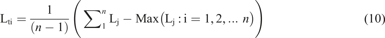
For the ALL_{inner trim} ensemble model the upper interval (Uit) is calculated by taking the average of the (n – 1) largest upper intervals, which is equal to the four largest upper intervals in our application of the model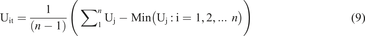

U_{i t} = \frac{1}{(n - 1)} (\sum_{1}^{n} U_{j} - Min (U_{j} : i = 1, 2, . . . n))

(9)

And the lower interval (Lit) is equal to the average of the (n – 1) smallest lower intervals, which is equal to the four smallest lower intervals in our application of the model

L_{t i} = \frac{1}{(n - 1)} (\sum_{1}^{n} L_{j} - Max (L_{j} : i = 1, 2, . . . n))

(10)

This method provides a more conservative interval than using a simple mean (Jose et al., 2013; Yaniv, 1997).

Error metrics

For each model we produce point, low and high forecasts, where the latter two represent the lower and upper bounds of the 80% prediction interval. 80% prediction intervals are commonly presented with probabilistic population forecasts, including those produced by the United Nations (e.g. United Nations, 2019). Accuracy of point forecasts is assessed using the absolute percentage error (APE), a standard metric used in population forecasting research (Rayer, 2007). At time t, the absolute percentage error (APE) equals

A P E = \frac{| F_{t} - A_{t} |}{A_{t}} \times 100

(11)

Where A_t is the actual population at time t and F_t is the mean population forecast at time t. The median Absolute Percentage Error (MedAPE) and the mean Absolute Percentage Error (MAPE) is used to summarise the APE across all small areas for each forecast horizon. Population forecasts generally produce APE distributions with a long tail of errors. The impacts of these errors is smaller on MedAPE than on the MAPE, therefore, we focus our analyses and discussion on the MedAPE.

We use two metrics to assess the accuracy of the prediction intervals. Coverage, which we report as the percentage of true values which fall within the 80% prediction intervals. Coverage is a simple and easy to understand metric which has previously been used in probabilistic forecast evaluations (Rayer et al., 2009; Sevcikova et al., 2018; Tayman et al., 2007). However, if a method produces very large prediction intervals, then this will produce large Coverage but unhelpful forecasts. Therefore, we also calculated the Mean Scaled Interval Score (MSIS; Gneiting and Raftery, 2007), which is a scale independent metric for the evaluation of prediction intervals. MSIS is based on the interval score developed by Gneiting and Raftery (2007), whose work is the basis of a significant portion of the literature evaluating probabilistic forecasts, including the evaluation of national probabilistic forecasts by Keilman et al., (2020), and of the probabilistic forecasts in the M4 competition (Makridakis et al., 2020).

The formula for the MSIS at time t is presented below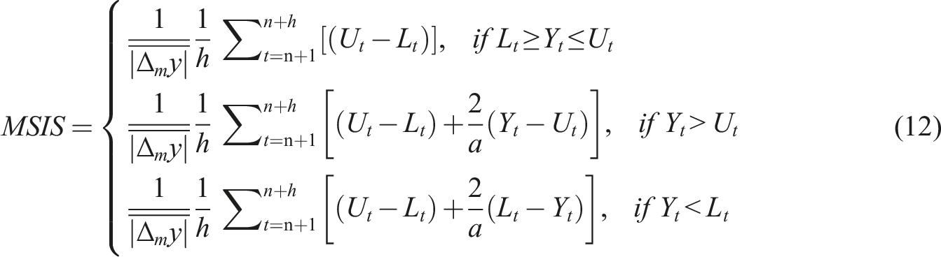

M S I S = {\begin{array}{c} \frac{1}{\bar{| ∆_{m} y |}} \frac{1}{h} \sum_{t = n + 1}^{n + h} [(U_{t} - L_{t})], i f L_{t} \geq Y_{t} \leq U_{t} \\ \frac{1}{\bar{| ∆_{m} y |}} \frac{1}{h} \sum_{t = n + 1}^{n + h} [(U_{t} - L_{t}) + \frac{2}{a} (Y_{t} - U_{t})], i f Y_{t} > U_{t} \\ \frac{1}{\bar{| ∆_{m} y |}} \frac{1}{h} \sum_{t = n + 1}^{n + h} [(U_{t} - L_{t}) + \frac{2}{a} (L_{t} - Y_{t})], i f Y_{t} < L_{t} \end{array}

(12)

where n is the length of the time series, and m is the frequency of the times series which is equal to one as our data is yearly. L_t is the lower bound of the prediction interval and U_t the upper bound. h is the forecast horizon; when we evaluate the 5 and 10 years forecasts, h is set as 5 and 10 respectively. Y_t is the actual value.

a

is the significance level which is 0.2 for our study as we present 80% prediction intervals. The calculation of MSIS is conditional, if the actual value falls outside the intervals an additional penalty is added to the score. MSIS is scale independent as the denominator is divided by the average seasonal difference over the length of the time series using the equation below (Castle et al., 2019).

\bar{| ∆_{m} y |} = \frac{1}{n - m} \sum_{t = m + 1}^{n} | Y_{t} - Y_{t - m} |

(13)

In our study the data is yearly, therefore, equation (13) gives the average absolute change in population from 1 year to the next over the base period. We calculate MSIS for each area and present the mean MSIS across areas.

The MSIS metric penalises methods which produce large intervals. However, we suggest that large intervals are not necessarily indicative of a bad model if those intervals are accurately showing that an area’s population is difficult to predict and that forecasts for it are likely to be erroneous. To investigate this, for each model, we consider the correlation between the absolute percentage errors of the point forecasts and the half-widths of its prediction intervals (Lee and Tuljapurkar, 1994).

Remoteness

Australian SA2 areas can be classified by their remoteness as major cities, inner regional, outer regional, remote and very remote (Australian Bureau of Statistics, 2013). Here we disaggregate our forecast results by remoteness and present tables containing the MedAPE, MAPE, Coverage, MSIS, Half-Widths and correlation between APEs of the point forecasts and the half-widths of the prediction intervals, for each remoteness area.

Results

Probabilistic forecast evaluation

Table 3 summarises the overall results of the probabilistic forecasting models for 5 and 10 years forecast horizons. The most accurate method in terms of MedAPE is the ALL model. The MedAPE for each of the three ALL ensemble variants are the same because the variants differ in how their intervals are calculated, not in how their point forecast is calculated. The ensemble models perform notably better than the individual models. The statistical models and GBMs perform similarly in terms of MedAPE.

Table 3.

SA2 total population forecast errors: An evaluation of point forecasts and prediction intervals, after 5 and 10 years.

	Statistical			Machine learning		Ensemble
	ARIMA	ETS	THETA	XGBOOST	LGBM	STAT	ALL average	ALL envelope	ALL Inner trim
MedAPE
After 5 years
2006-based	4.09	4.23	4.62	4.43	4.33	3.94	3.91	3.91	3.91
2011-based	3.77	3.60	3.85	3.75	3.70	3.40	3.24	3.24	3.24
After 10 years
2006-based	7.53	7.73	7.86	7.94	7.64	6.96	6.56	6.56	6.56
MAPE
After 5 years
2006-based	5.87	5.89	6.68	6.58	6.34	5.60	5.56	5.56	5.56
2011-based	5.78	5.42	5.94	6.10	6.19	5.18	5.26	5.26	5.26
After 10 years
2006-based	10.63	10.66	11.11	11.63	11.50	9.77	9.32	9.32	9.32
Coverage (%)
After 5 years
2006-based	54.94	52.95	45.55	24.59	26.72	56.10	49.13	73.38	56.58
2011-based	56.92	65.44	54.07	49.37	46.95	64.96	63.07	84.85	70.62
After 10 years
2006-based	56.00	54.31	40.90	24.20	29.57	57.41	52.32	79.38	61.91
MSIS
After 5 years
2006-based	23.42	24.45	27.53	31.75	32.12	23.31	24.91	21.04	23.40
2011-Based	18.16	16.26	19.53	20.31	20.19	15.99	16.00	15.52	15.22
After 10 years
2006-Based	45.17	47.38	53.51	53.47	56.59	44.34	44.19	38.70	41.69
Half-width
After 5 years
2006-based	6.33	7.11	5.85	3.01	2.98	6.44	5.09	10.76	6.38
2011-based	5.91	7.80	5.52	4.29	4.02	6.42	5.55	11.10	6.79
After 10 years
2006-based	14.38	15.56	7.96	4.30	4.82	12.55	9.47	23.21	12.24
Correlation
After 5 years
2006-based	0.36	0.30	0.42	0.44	0.43	0.39	0.44	0.46	0.46
2011-based	0.41	0.30	0.41	0.50	0.51	0.44	0.52	0.48	0.52
After 10 years
2006-based	0.22	0.25	0.50	0.17	0.31	0.31	0.33	0.31	0.34

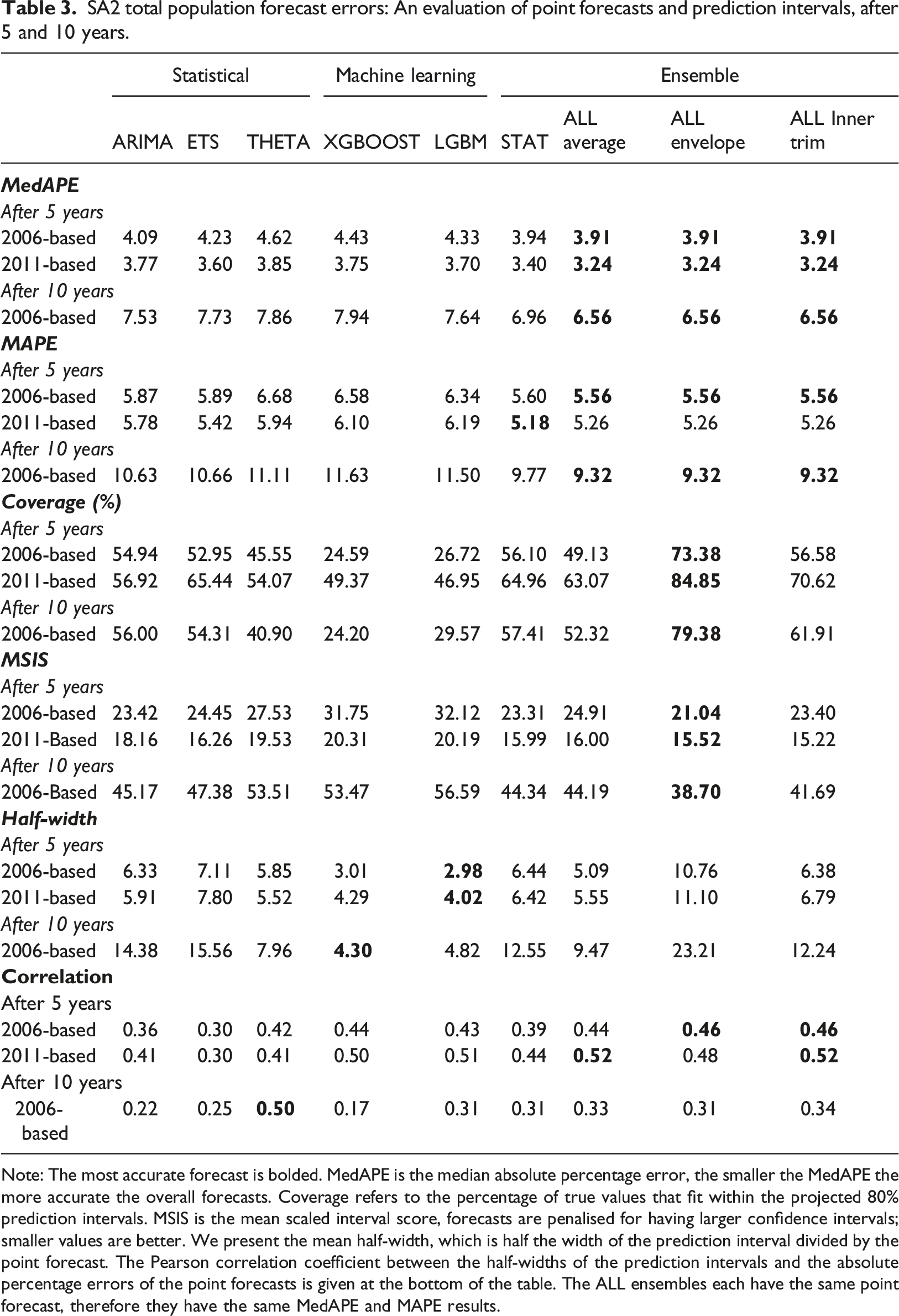
Note: The most accurate forecast is bolded. MedAPE is the median absolute percentage error, the smaller the MedAPE the more accurate the overall forecasts. Coverage refers to the percentage of true values that fit within the projected 80% prediction intervals. MSIS is the mean scaled interval score, forecasts are penalised for having larger confidence intervals; smaller values are better. We present the mean half-width, which is half the width of the prediction interval divided by the point forecast. The Pearson correlation coefficient between the half-widths of the prediction intervals and the absolute percentage errors of the point forecasts is given at the bottom of the table. The ALL ensembles each have the same point forecast, therefore they have the same MedAPE and MAPE results.

The Coverage of our 80% prediction intervals is shown below MedAPE in Table 3. Coverage was less than 80% for all methods except ALL_envelope, thus for most methods the prediction intervals did not adequately forecast the range where actual populations would be. The statistical methods produced better Coverage than the GBMs. The ALL_envelope model produced the best MSIS results.

Half-widths for XGBOOST and LGBM are notably smaller than for the other methods, explaining why their Coverage is smaller despite comparable MedAPEs. As expected, the ALL_envelope model produces forecasts with the largest intervals. THETA had the narrowest intervals of the individual statistical methods.

Correlations of the absolute percentage errors of a model’s point forecasts and the size of its half widths are shown at the bottom of Table 3. THETA consistently produced correlations between 0.4 and 0.5, suggesting that the size of its intervals gives forecast users a better estimate of forecast uncertainly relative to the other models considered, however, it still isn’t able to account for most small area forecast uncertainty.

Figure 2 visualises 10 years 2006-based forecasts for the Bellingen SA2, an outer regional area in New South Wales. This visualisation indicates that methods which produce wider intervals in the first few years of a forecast may differ to those that produce wider intervals in the longer term. THETA produces relatively conservative intervals for Year one of the forecast and may be appropriate for probabilistic nowcasting (refer to Tables S1 to S6 of the Supplementary Materials for results for all forecast horizons).

Figure 2.

2006-based 10 years forecasts for the Bellingen SA2 area. Note: Figures show forecasts with 80% prediction intervals indicated in light blue.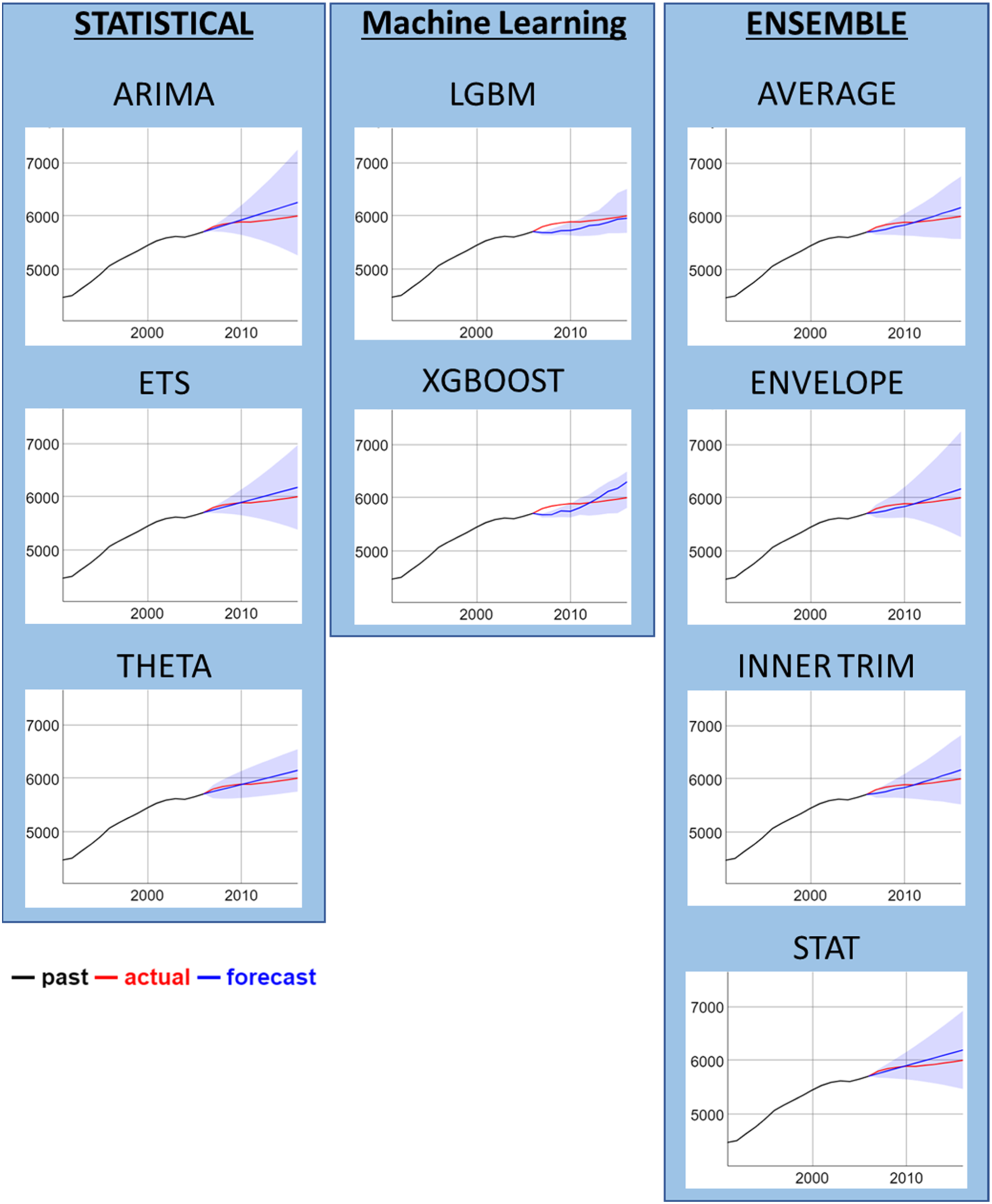

Remoteness

Previous research has shown that the accuracy of deterministic forecasts tends to be less for remote and very remote areas (Wilson and Rowe, 2011; Wilson et al., 2021b). We investigated whether remoteness influences the performance of both point forecasts and interval forecasts. These results are presented in the supplementary material, as Tables S7 to S12.

Tables S7 presents the MedAPEs for the SA2 total population point forecasts. The ensemble models tend to outperform the individual models for major cities and inner regional areas. However, the benefit of ensembling for the MedAPE score is less clear for more remote areas where individual models often perform better, particularly THETA. When we compare MedAPEs for the STAT and ALL_average models the results indicate that the inclusion of Machine Learning models using a simple mean combination method tended to increase forecast accuracy for Major cities, however, there was no clear pattern for other remoteness areas. There is a ‘U’ shaped relationship between remoteness and forecast accuracy. Accuracy tends to be better for regional areas than for SA2s in major cities, remote areas, or very remote areas. The ‘U’ is asymmetrical, with the accuracy of forecasts for very remote areas being notably worse than for major cities. The MAPE results by remoteness are presented in Table S8. They are similar to the MEDAPE results, albeit the Remote areas have particularly high MAPEs for the 2006-based 10 years forecasts.

Table S9 presents Coverage by remoteness for the prediction intervals. For the 5 years forecasts, Coverage tends to be worst for more remote areas. After 10 years, the Coverage of the prediction intervals tends to be worst for major cities. Using simple mean interval combination methods did not improve coverage to desired 80% levels and the inclusion of the Machine Learning forecasts tended to decrease forecast accuracy, thus the STAT model tends to have slightly better coverage than the ALL_average model. ALL_envelope is the only model to consistently generate prediction intervals that cover approximately 80% of actual values across remoteness levels, jump-off years and forecast horizons (range: 65.96%–90.85%). All other models always underestimate forecast uncertainty.

MSIS is presented in Table S10. The ensemble methods tended to perform better than the other statistical methods, particularly ALL_envelope. The ML methods tended to have relatively poor MSIS scores. Most models performed relatively poorly for Major Cities for the 2006-based 10 years forecasts.

Table S11 presents the mean half widths of the 80% prediction intervals by remoteness. LGBM and XGBOOST have the smallest half widths. As expected by its construction, the ALL_envelope model has the largest prediction intervals across remoteness areas. Across the models, the half-widths tend to be greatest for very remote areas and smallest for the inner regional and outer regional SA2s.

Table S12 presents the correlations between the APEs generated by the point forecasts, and the half widths of the prediction intervals, for each of the remoteness levels. The models which produce the highest correlations vary depending on the jump-off year, forecast horizon and remoteness. None of the models produce reliably high correlations across the remoteness areas.

Discussion

In this study, we have investigated and evaluated the use of probabilistic models for small area population forecasting. This context requires stochastic forecasting methods to be developed and implemented due to the high uncertainty present. We considered five individual probabilistic forecasting models and four ensemble models. Our overall results indicate that ensemble models performed better when they included both statistical models and globally trained GBMs. However, an analysis by remoteness found that whilst GBMs improved the performance of ensemble models for SA2s in major cities, they did not improve performance for remote and very remote areas. We discuss these findings below, how they addressed our aims, explore issues related to model-based prediction intervals, consider the limitations and implications of this study.

Our first aim was to evaluate the performance of individual probabilistic models, which included statistical models and GBMs. Of these, ARIMA and ETS produced point forecasts with the smallest MedAPEs, and 80% prediction intervals with the highest Coverage, for the 2006- and 2011- based forecasts, respectively. However, the coverage of the best performing individual methods (54%–65%) was still significantly smaller than what may be expected from 80% prediction intervals. The GBMs did not perform particularly well in our study. Whilst their point forecasts were relatively accurate, coverage was poor for their interval forecasts. Conversely, the top performing methods in the M5 uncertainty competition utilised LGBM methods (Makridakis et al., 2021). The M5 competition dataset contains daily hierarchical retail sales time series data, which are longer than the yearly time series in our small area dataset and additional explanatory variables were used to develop the models. However, the results of the M5 uncertainty competition showed that the benefit of the LGBM based methods, relative to their benchmark ARIMA model, were most evident at the higher levels of the hierarchy; the benefit was limited at the lowest levels (Makridakis et al., 2021). Thus, GBM based methods may be more useful for forecasting populations at higher geographical scales.

Our second aim was to investigate methods to combine the forecasts produced by our individual probabilistic models. The overall MedAPEs of the Ensemble models were considerably lower than those of the individual models. Indeed, the ALL ensemble produced more accurate point forecasts in terms of MedAPE than all bar one of the unconstrained results found in an evaluation of the top M4 competition methods for point forecasts of Australian SA2 small areas (Wilson et al., 2021b). Overall, the ALL_average model performed better than the STAT model, indicating that it was advantageous to include the GBMs in the ensemble. This is in line with previous work investigating combination methods for small area population point forecasts (Grossman et al., 2022).

Our third aim was to investigate how the remoteness of small areas impacted the performance of the point forecasts and prediction intervals. Across all models, forecasts are generally more accurate and have better Coverage for regional areas than for major cities or more remote areas. Similar results were found in an evaluation of deterministic methods for Australian SA2s in Wilson et al., (2021b), however, results were different for New Zealand with Major Urban and Rural areas generally having smaller MedAPEs than Medium and Small urban areas. Whilst our overall results indicate that the addition of GBMs to ensemble models improves forecast performance, analysis by remoteness found that this is only consistently true for major cities. SA2s in major cities make up 1187 of the 2066 time series in the dataset. Conversely there were only 47 remote areas and 50 very remote areas. Therefore, it is unsurprising that the GBM forecasts are not as helpful for more remote areas, as they were not well represented by the training set.

Model-based prediction intervals routinely underestimate forecast uncertainty. This is a well-documented phenomenon, it was one of our findings, and one of the results of the M4 competition (Makridakis et al., 2018). Hyndman et al. (2002) found that the 95% Prediction intervals generated by Exponential Smoothing Methods covered between 71.1 to 87.5% of the series’ true values. The reasons for this attribute of prediction intervals relate to there being multiple sources of uncertainty that impact the performance of forecasts. Hyndman (2014) lists four: random error, parameter estimates, model choice and the uncertainty related to whether the processes which generate the data will change in the forecast period. The intervals generated by probabilistic forecasting models generally only address the uncertainty linked with the error term (Hyndman, 2014). Using an ensemble model approach can help address some of the uncertainty linked with the choice of model. Overall, our ensemble models tended to be more accurate and provided better Coverage than the individual models. ALL_envelope is the only model which achieved Coverage at the desired 80% level with relatively wide prediction intervals which had half-widths of approximately 10% of the point forecast after 5 years and 20% after 10 years. Whilst other models produced narrower intervals, this came at the cost of understating the level of uncertainty associated with their predictions. Bryant and Zhang (2016) used a Bayesian approach to create probabilistic forecasts for New Zealand small area emigration rates. Their 50% and 90% intervals covered 58% and 90.6% of the true values respectively. Their intervals were large, but they argued that this is necessary given that long-term forecasting is uncertain, and it prompts ‘users to confront the substantial uncertainty about long-term trends’ (Bryant and Zhang, 2016, p. 1337).

Conclusions

Given the inherent uncertainty in small area population forecasting, it is important to provide users with an indication of forecast uncertainty. In this study, we evaluated five individual and four ensemble models for probabilistic small area population forecasts. The individual probabilistic models produced prediction intervals that cover less than the desired 80% of true values. This is a known issue for model-based prediction intervals. We show that combination methods such as the inner trim and envelope techniques can improve Coverage. Ensemble models which included both statistical models and GBMs tended to outperform individual models for both point forecasts and prediction intervals. However, when we disaggregated the forecast results by the remoteness of the small areas, we found that the inclusion of GBMs in ensemble models was only beneficial for major cities. Practitioners using global models should consider if areas of interest are represented by the wider dataset and investigate the use of additional variables.

One of the limitations of this work is that we only evaluated our models using an Australian SA2 dataset. It is important to investigate how models perform across multiple datasets before recommendations can be made to practitioners about which probabilistic models to use. In turn, it is important for practitioners to help researchers understand what the requirements for the intervals are, and how they will be used.

Supplemental Material

Supplemental Material - Development and evaluation of probabilistic forecasting methods for small area populations

Supplemental Material for Development and evaluation of probabilistic forecasting methods for small area populations by Irina Grossman, Kasun Bandara, Tom Wilson, and Michael Kirley in Environment and Planning B: Urban Analytics and City Science

Footnotes

Declaration of conflicting interests

The author(s) declared no potential conflicts of interest with respect to the research, authorship, and/or publication of this article.

Funding

The author(s) disclosed receipt of the following financial support for the research, authorship, and/or publication of this article: This research was funded by the Australian Government through the through the Australian Research Council’s Discovery Projects funding scheme (Project DP200101480).

Data availability

Data is available at:

ORCID iDs

Irina Grossman

Kasun Bandara

Supplemental Material

Supplemental material for this article is available online.

Irina Grossman is a Postdoctoral Researcher at the Melbourne School of Population and Global Health at the University of Melbourne. She received her PhD in cognitive neuroscience and has a Bachelor of Science and a Bachelor of Engineering (first class hons) in the field of electrical and computer systems. Her current research interests are in macro-demographic dynamics, particularly population forecasting methods.

Kasun Bandara received the B.Sc. honours degree in Computer Science from the University of Colombo School of Computing, Sri-Lanka, in 2015 and the Ph.D. degree in Computer Science from Monash University, Australia in 2020. He is currently working as a Forecast Analytics Analyst at EnergyAustralia and an Honorary Research Fellow at the Melbourne Centre for Data Science at The University of Melbourne, Australia. His research interests include Big Data, deep neural networks and time series forecasting.

Tom Wilson is a Principal Research Fellow at the Melbourne School of Population and Global Health at the University of Melbourne. His current research interests are in population projections, migration analysis, indirect estimation, household modelling, advanced age populations, regional and local population change, Indigenous demography, and LGBTQ demography.

Michael Kirley is the Co-Director of the Melbourne Centre for Data Science and a Professor in the School of Computing and Information Systems at the University of Melbourne. His current research interests include artificial intelligence, machine learning techniques, and game theory.

References

Assimakopoulos

Nikolopoulos

(2000) The theta model: a decomposition approach to forecasting. International Journal of Forecasting 16(4): 521–530.

Australian Bureau of Statistics (2013) 1270.0.55.005 - Australian Statistical Geography Standard (ASGS): Volume 5 - Remoteness Structure, July 2011. Available at: https://www.abs.gov.au/AUSSTATS/abs@.nsf/allprimarymainfeatures/17A7A350F48DE42ACA258251000C8CA0?opendocument

Australian Bureau of Statistics (2017a). ERP by SA2 and above (ASGS 2011), 1991 to 2016. Available at: http://stat.data.abs.gov.au/Index.aspx?DataSetCode=ABS_ANNUAL_ERP_ASGS

Australian Bureau of Statistics (2017b) 3218.0 - Regional Population Growth, Australia, 2016. Available at: https://www.abs.gov.au/AUSSTATS/abs@.nsf/Lookup/3218.0Explanatory%20Notes12016?OpenDocument

Azose

Ševčíková

Raftery

(2016) Probabilistic population projections with migration uncertainty. Proceedings of the National Academy of Sciences of the United States of America 113(23): 6460–6465.

Bandara

Bergmeir

Campbell

, et al. (2020) Towards accurate predictions and causal ‘what-if’analyses for planning and policy-making: a case study in emergency medical services demand. 2020 International Joint Conference on Neural Networks (IJCNN). Glasgow, UK: IEEE, 1–10.

Ben Taieb

Bontempi

Atiya

, et al. (2012) A review and comparison of strategies for multi-step ahead time series forecasting based on the NN5 forecasting competition. Expert Systems with Applications 39(8): 7067–7083.

Bergstra

Yamins

Cox

(2013) Making a science of model search: Hyperparameter optimization in hundreds of dimensions for vision architectures. 30th International Conference on International Conference on Machine Learning - Volume 28. Atlanta, GA, USA: JMLR.org, 115–123. ISBN.

Box

Jenkins

Reinsel

, et al. (2015) Time Series Analysis: Forecasting and Control. Hoboken, New Jersey: John Wiley and Sons.

10.

Breiman

(2001) Random forests. Machine Learning 45(1): 5–32.

11.

Bryant

Graham

(2013) Bayesian Demographic Accounts: Subnational Population Estimation Using Multiple Data Sources. Bayesian Analysis 8(3): 591–622.

12.

Bryant

Zhang

(2016) Bayesian forecasting of demographic rates for small areas: emigration rates by age, sex, and region in New Zealand, 2014-2038. Statistica Sinica 26: 1337–1363.

13.

Castle

Doornik

Hendry

(2019) Some forecasting principles from the M4 competition. In: Nuffield College. Oxford: University of Oxford.

14.

Chen

Guestrin

(2016) Xgboost: a scalable tree boosting system. Proceedings of the 22nd Acm Sigkdd International Conference on Knowledge Discovery and Data Mining. New York, NY, United States: Association for Computing Machinery, 785–794.

15.

De Beer

(1997) The effect of uncertainty of migration on national population forecasts: the case of the Netherlands. Journal of Official Statistics-Stockholm 13: 227–244.

16.

Genre

Kenny

Meyler

, et al. (2013) Combining expert forecasts: can anything beat the simple average? International Journal of Forecasting 29(1): 108–121.

17.

Gneiting

Raftery

(2007) Strictly proper scoring rules, prediction, and estimation. Journal of the American Statistical Association 102(477): 359–378.

18.

Grossman

Bandara

Wilson

, et al. (2022) Can machine learning improve small area population forecasts? A forecast combination approach. Computers, Environment and Urban Systems 95: 101806.

19.

Grushka-Cockayne

Jose

VRR

(2020) Combining prediction intervals in the m4 competition. International Journal of Forecasting 36(1): 178–185.

20.

Hewamalage

Bergmeir

Bandara

(2021) Global models for time series forecasting: a simulation study. Pattern Recognition 124: 108441. DOI: 10.1016/j.patcog.2021.108441

21.

Hyndman

Athanasopoulos

Bergmeir

, et al. (2022) Package ‘forecast’. Available at: https://cran.r-project.org/web/packages/forecast/forecast.pdf

22.

Hyndman

(2014) Prediction intervals too narrow. Available at: https://robjhyndman.com/hyndsight/narrow-pi/(accessed 29 04 2022).

23.

Hyndman

Billah

(2003) Unmasking the theta method. International Journal of Forecasting 19(2): 287–290.

24.

Hyndman

Khandakar

(2008) Automatic time series forecasting: the forecast package for R. Journal of Statistical Software 27: 1–22.

25.

Hyndman

Koehler

Snyder

, et al. (2002) A state space framework for automatic forecasting using exponential smoothing methods. International Journal of Forecasting 18(3): 439–454.

26.

Januschowski

Wang

Torkkola

, et al. (2022) Forecasting with trees. International Journal of Forecasting 38: 1473–1481.

27.

Jiang

Jin

Liu

, et al. (2007) A HMM-Based Hierarchical Framework for Long-Term Population Projection of Small Areas. Berlin, Heidelberg: Springer Berlin Heidelberg, pp. 694–698.

28.

Jose

VRR

Grushka-Cockayne

Lichtendahl

Jr (2014) Trimmed opinion pools and the crowd’s calibration problem. Management Science 60(2): 463–475.

29.

Meng

Finley

, et al. (2017) LightGBM: A Highly Efficient Gradient BoostingDecision Tree. NIPS’17: Proceedings of the 31st International Conference on Neural Information Processing System. Red Hook, NY, United States: Curran Associates Inc., 3149–3157.

30.

Meng

Finley

Wang

Chen

Liu

(2021) LightGBM. Microsoft Corporation. Available at: https://lightgbm.readthedocs.io/

31.

Keilman

(2020) Évaluer les prévisions probabilistes de population/evaluating probabilistic population forecasts. Economie et Statistique 520(1): 51–68.

32.

Keilman

Pham

Hetland

(2002) Why population forecasts should be probabilistic - illustrated by the case of Norway. Demographic Research 6: 409–454.

33.

Keyfitz

(1981) The limits of population forecasting. Population and Development Review 7: 579–593.

34.

Lee

Tuljapurkar

(1994) Stochastic population forecasts for the united states: beyond high, medium, and low. Journal of the American Statistical Association 89(428): 1175–1189.

35.

Makridakis

Hibon

(2000) The M3-competition: results, conclusions and implications. International Journal of Forecasting 16(4): 451–476.

36.

Makridakis

Spiliotis

Assimakopoulos

(2018) The M4 competition: results, findings, conclusion and way forward. International Journal of Forecasting 34(4): 802–808.

37.

Makridakis

Spiliotis

Assimakopoulos

(2020) The M4 competition: 100,000 time series and 61 forecasting methods. International Journal of Forecasting 36(1): 54–74.

38.

Makridakis

Spiliotis

Assimakopoulos

(2022) M5 accuracy competition: results, findings, and conclusions. International Journal of Forecasting 38: 1346–1364.

39.

Makridakis

Spiliotis

Assimakopoulos

, et al. (2022) The M5 Uncertainty competition: results, findings and conclusions. International Journal of Forecasting 38: 1365–1385.

40.

Okita

Pfau

Long

(2011) A stochastic forecast model for Japan's population. Japanese Economy 38(2): 19–44.

41.

Pedregosa

Varoquaux

Gramfort

, et al. (2011) Scikit-learn: machine learning in python. Journal of Machine Learning Research 12: 2825–2830.

42.

Queensland Government Statistician’s Office (2019) Understanding population statistics. Available at: https://www.qgso.qld.gov.au/about-statistics/analysing-data/understanding-population-statistics

43.

Rayer

(2007) Population forecast accuracy: does the choice of summary measure of error matter? Population Research and Policy Review 26: 163.

44.

Rayer

Smith

Tayman

(2009) Empirical prediction intervals for county population forecasts. Population Research and Policy Review 28(6): 773–793.

45.

Schapire

(1999) A brief introduction to boosting. In: Proceedings of the 16th International Joint Conference on Artificial Intelligence. San Francisco, CA, USA: Morgan Kaufmann Publishers Inc., pp. 1401–1406.

46.

Setiawan

Sukamdi Listyaningsih

(2021) Probabilistic population projections for provincial levels in Indonesia. Journal of Physics: Conference Series. Bogor, Indonesia: IOP Publishing, 012011.

47.

Sevcikova

Raftery

Gerland

(2018) Probabilistic projection of subnational total fertility rates. Demographic Research 38: 1843–1884.

48.

Simpson

Wilson

Shalley

(2020) The shelf life of official sub-national population forecasts in England. Applied Spatial Analysis and Policy 13(3): 715–737.

49.

Statistics New Zealand (2016) How accurate are population estimates and projections? An evaluation of Statistics New Zealand population estimates and projections, 1996 - 2013. Statistics New Zealand. Wellington, New Zealand: Statistics New Zealand.

50.

Tayman

(2011) Assessing Uncertainty in Small Area Forecasts: State of the Practice and Implementation Strategy. Population Research and Policy Review 30: 781–800.

51.

Tayman

Smith

Lin

(2007) Precision, bias, and uncertainty for state population forecasts: an exploratory analysis of time series models. Population Research and Policy Review 26(3): 347–369.

52.

Timmermann

(2006) Chapter 4 forecast combinations. In: Elliott

Granger

CWJ

Timmermann

(eds). Handbook of Economic Forecasting. Amsterdam; Boston: Elsevier North-Holland, 135–196.

53.

United Nations (2019) World Population Prospects 2019. Department of Economic and Social Affairs PD. New York: United Nations.

54.

Wilson

Bell

(2004) Australia’s uncertain demographic future. Demographic Research 11: 195–234.

55.

Wilson

Bell

(2007) Probabilistic regional population forecasts: the example of Queensland, Australia. Geographical Analysis 39(1): 1–25.

56.

Wilson

, Brokensha

, Rowe

, et al. (2018) Insights from the evaluation of past local area population forecasts. Population Research and Policy Review 37: 137–155

57.

Wilson

Machado

Sousa

DER

, et al. (2021a) Methods for small area population forecasts: state-of-the-art and research needs. Journal of the American Veterinary Medical Association 259: 1–3.

58.

Wilson

Grossman

Temple

(2023) Evaluation of the best M4 competition methods for small area population forecasting. International Journal of Forecasting 39: 110–122. DOI: 10.1016/j.ijforecast.2021.09.005

59.

Wilson

Rowe

(2011) The forecast accuracy of local government area population projections: a case study of Queensland. Australasian Journal of Regional Studies 17: 204–243.

60.

Yaniv

(1997) Weighting and trimming: heuristics for aggregating judgments under uncertainty. Organizational Behavior and Human Decision Processes 69(3): 237–249.

61.

Zhang

Bryant

(2020) Bayesian disaggregated forecasts: internal migration in Iceland. In: Developments in Demographic Forecasting. Cham: Springer, pp. 193–215.

Supplementary Material

Please find the following supplemental material available below.

For Open Access articles published under a Creative Commons License, all supplemental material carries the same license as the article it is associated with.

For non-Open Access articles published, all supplemental material carries a non-exclusive license, and permission requests for re-use of supplemental material or any part of supplemental material shall be sent directly to the copyright owner as specified in the copyright notice associated with the article.

0.00 MB

0.56 MB