Sage Journals: Discover world-class research

Abstract

We study the compositional and configurational heterogeneity of Greater London at the city- and neighbourhood-scale using Geographic Information System (GIS) data. Urban morphometric indicators are calculated including plan-area indices and fractal dimensions of land cover, frontal area index of buildings, evenness, and contagion. To distinguish between city-scale heterogeneity and neighbourhood-scale heterogeneity, the study area of 720 km² is divided into 1 $\times$ 1 km² neighbourhoods. City-scale heterogeneity is represented by categorisation of the neighbourhoods using a k-means clustering algorithm based on the morphometric indicators. This results in six neighbourhood types ranging from “greenspace” to “central business district”. Neighbourhood-scale heterogeneity is quantified using a hierarchical multi-scale analysis for each neighbourhood type. The analysis reveals the dominant length scales for land-cover and neighbourhood types and the resolutions with the most information gain. We analyse multi-scale anisotropy and show that small-scale features are homogeneous, and that anisotropy is present at larger length scales.

Keywords

spatial heterogeneity urban landscape neighbourhood-scale classification

Introduction

The urban landscape, a patchwork of buildings, roads, pavements, gardens, parks, and water, is inherently heterogeneous. Although straightforward to understand intuitively, heterogeneity lacks a universally adopted definition, as it represents unevenness, randomness, difference, variability, complexity, and deviation from a norm. The Oxford English Dictionary defines heterogeneity as the difference or diversity in contrast with other things or being made up of things or parts differing greatly from each other (Fitch et al., 2015). Li and Reynolds (1995) define heterogeneity as ‘the complexity and/or variability of a system property in space and/or time’ (p. 280). Santos et al. (2021) distinguish between structural and functional heterogeneity. Structural heterogeneity relates to the size, quantity, and spatial configuration of different surface properties. Functional heterogeneity refers to quality and resource availability that affects ecological processes and responses, e.g., living organisms’ density and distribution. Heterogeneity also has a temporal component: the urban landscape is subject to abrupt, short-term, and long-term changes in its functional use and land-cover properties due to human activities, phenological cycles, and urbanisation of previously rural landscapes (Santos et al., 2021).

Heterogeneity in urban systems is created and maintained by many different processes across physical, biological and social realms. Physical processes involve natural progression, disturbances (e.g., fire, flood, etc.) and recovery, which set the heterogeneity of urban system at coarse scale. Biological processes refer to the interactions among organisms including humans, such as the competing for resources, resulting in the heterogeneity in population sizes and occupied locations (Pickett et al., 2000; Cadenasso et al., 2013). Social processes are related to the management, planning and design interventions by humans, modifying the physical structures and components of the urban system such as removing materials or transferring materials from one landscape to another, which leads to contrasting land covers and creates local areas differing from adjacent ones (Pastor, 2005; Pickett and Cadenasso, 2009; Cadenasso et al., 2013).

Heterogeneity of landscape properties plays an important role in the ecological processes and functioning of urban systems (Cadenasso et al., 2007, 2013). The built environment consists of a rich variety of materials and textures: common building materials are brick, stone, concrete, wood, and glass; building facades can be smooth, rough, or vegetated; roads are paved with asphalt or stones. These materials differ in their permeability, their capacity to store heat, absorb water or reflect solar radiation, and therefore influence the surface energy budget of urban environments (Oke et al., 2017). The density of buildings and street networks that run throughout a city may differ substantially for different areas. Densely built-up areas reduce the sky-view-factor and thus block the emission of thermal radiation. Continuous wide streets promote ventilation, which removes heat and air pollution from urban environments. The abundance or lack of urban vegetation and water also affect the urban energy budget on the neighbourhood scale (Zipper et al., 2017). The differences in structure and land-cover between urban and rural areas result in generally higher air temperatures in urban environments compared to the rural surroundings (Bohnenstengel et al., 2011), a phenomenon called the urban heat island (UHI; Buyantuyev and Wu, 2010; Qian et al., 2020; Stewart and Oke, 2012). The presence of the UHI has motivated research about how to assess and mitigate urban heat stress. For example, Bartesaghi Koc et al. (2020) identified different types of green infrastructure and their cooling capacity in Sydney, Australia by their morphological and spatial characteristics. As cities consist of neighbourhoods with different form and functionality, the heat island intensity varies spatially across the city, as does the distribution of air pollution (NOx, particulate matter) and anthropogenic heat from heating/cooling, industrial processes, and car engines (Allen et al., 2010; Crippa et al., 2021). Spatial heterogeneity has been a key concern for linking ecological sciences and urban design professions (Cadenasso et al., 2013; Pickett et al., 2017; Zhou et al., 2017).

Successful understanding of spatial heterogeneity in cities relies on its accurate quantification (Murwira, 2003). The quantification of urban heterogeneity not only provides a way to describe, assess and compare the morphologies of different urban landscapes, but also helps us understand how the physical characteristics of landscapes respond to urbanization or human manipulation (Cadenasso et al., 2013; Wiese et al., 2021). Heterogeneity can be quantified by measuring complexity and variability of a system property, and by measuring departure from homogeneity (Fitch et al., 2015; Li and Reynolds, 1995; Oke et al., 2017). There are numerous indices to assess heterogeneity of a landscape, each emphasizing a different aspect or property of the landscape.

Our study is motivated by providing a better representation of cities in global weather and climate models and thus the need to incorporate surface heterogeneity into atmospheric models due to the strong interaction between the land surface and the atmospheric boundary layer (Barlow, 2014; Margairaz et al., 2020; Oke et al., 2017). Indeed, the physical processes in the near-surface atmosphere are fundamentally related to urban morphology. For example, aerodynamic roughness is commonly estimated by geometric parameters including average surface element height, plan area index, and frontal area index (cf. Kent et al., 2017). Land-surface model components of atmospheric models, such as JULES (Best et al., 2011; Clark et al., 2011) and the Town-Energy-Balance model (TEB, Masson, 2000) rely on urban morphology indicators in order to make predictions of aerodynamic drag, sensible and latent heat fluxes, which characterise the influence of the surface on the atmospheric flow.

However, land-surface models use simplified representations of the urban surface and usually do not consider the spatial configuration of different surface types within the given area, even though it is known that the way the surface types are arranged within an urban area can have a profound effect on the interaction with the atmosphere (Bartesaghi Koc et al., 2020; Sützl et al., 2021a, 2021b). To improve these models, it is necessary to add information about the structural heterogeneity of the urban area to the model. This paper explores several indicators of heterogeneity that could serve this purpose, namely the fractal dimension, contagion, and evenness.

Another challenge for modelling urban climate is that heterogeneity is inherently multi-scale. An urban area may be spatially homogeneous in respect of a particular surface property at one length scale and heterogeneous at another (Oke et al., 2017). Before one can understand how the atmosphere is influenced by urban heterogeneity, it is crucial to define heterogeneity in a multi-scale context. This is particularly pertinent in the context of numerical weather prediction, where the increase in computational resources has allowed simulation at higher and higher resolution over the years (Jochem et al., 2021). For example, the UK Met Office now runs its main weather forecasting model at a grid of 1500 m (Tang et al., 2013), and experiments with resolutions even of the order of hundreds of metres (Boutle et al., 2016; Lean et al., 2019). With each increase in the resolution, part of the surface heterogeneity which was sub-grid (at scales smaller than the grid size) becomes resolved which will then affect the atmospheric flow. For an ideal model, predictions would be independent of resolution. In this paper, we develop a hierarchical decomposition at neighbourhood level that is able to quantify the effect of changes in resolution on heterogeneity.

The aim of this paper is to use high-resolution land-use data of Greater London to explore how structural heterogeneity can be defined in a multi-scale setting, making use of spatial maps of land-cover types, their spatial aggregation and fractal dimensions, distinguishing between city-scale heterogeneity and neighbourhood-scale heterogeneity. The Greater London area includes rural, suburban, and urban areas, as well as large parks and water bodies (e.g., the river Thames). Firstly, the city-scale heterogeneity is captured through land-cover and urban function categories based on a $k$ -means clustering algorithm. Clustering methods have been used extensively in urban morphological studies (Fleischmann et al., 2021), to classify building types (Berghauser Pont et al., 2019), settlement types (Jochem and Tatem, 2021; Jochem et al., 2021), sanctuary areas (Dibble et al., 2019) and morphological cells (Fleischmann et al., 2021). Secondly, neighbourhood-scale heterogeneity will be investigated using a novel hierarchical decomposition method. Finally, conclusions are made in the last section.

Methodology

Study area and map sources

The study area covers most of Greater London on 24 $\times$ 30 km², ranging from 515000, 169000 to 545000, 193000 in British National Grid (EPSG:27700) reference system. The map data are supplied by Digimap Ordnance Survey, including vector layer (Ordnance Survey (GB) 2020a), raster layer (Ordnance Survey (GB) 2017) and Building Height Attribute data (Ordnance Survey (GB) 2020b). The vector map consists of twenty-seven land features, such as buildings, structures, land, inland water, rail, paths and roads. This study categorizes all land features to four main land-cover types, namely buildings (including structures), impervious (including roads, rail and other impervious ground surfaces), vegetation, and water, summarised in Table S1. The original raster map at pixel resolution of 0.3125 m is also reclassified into four land-cover types using vector layer in QGIS software. The reclassified land-cover raster map is shown in Figure 1, where each colour represents a different land-cover type.

Figure 1.

Reclassified land-cover raster map of the study area with four categories: buildings and structures (black), impervious surface (pink), vegetation (green), and water (dark blue). A spatial reference of the area is shown in the insert map (red rectangle). National and Greater London outlines from the Boundary-Line data (Ordnance Survey (GB) 2021).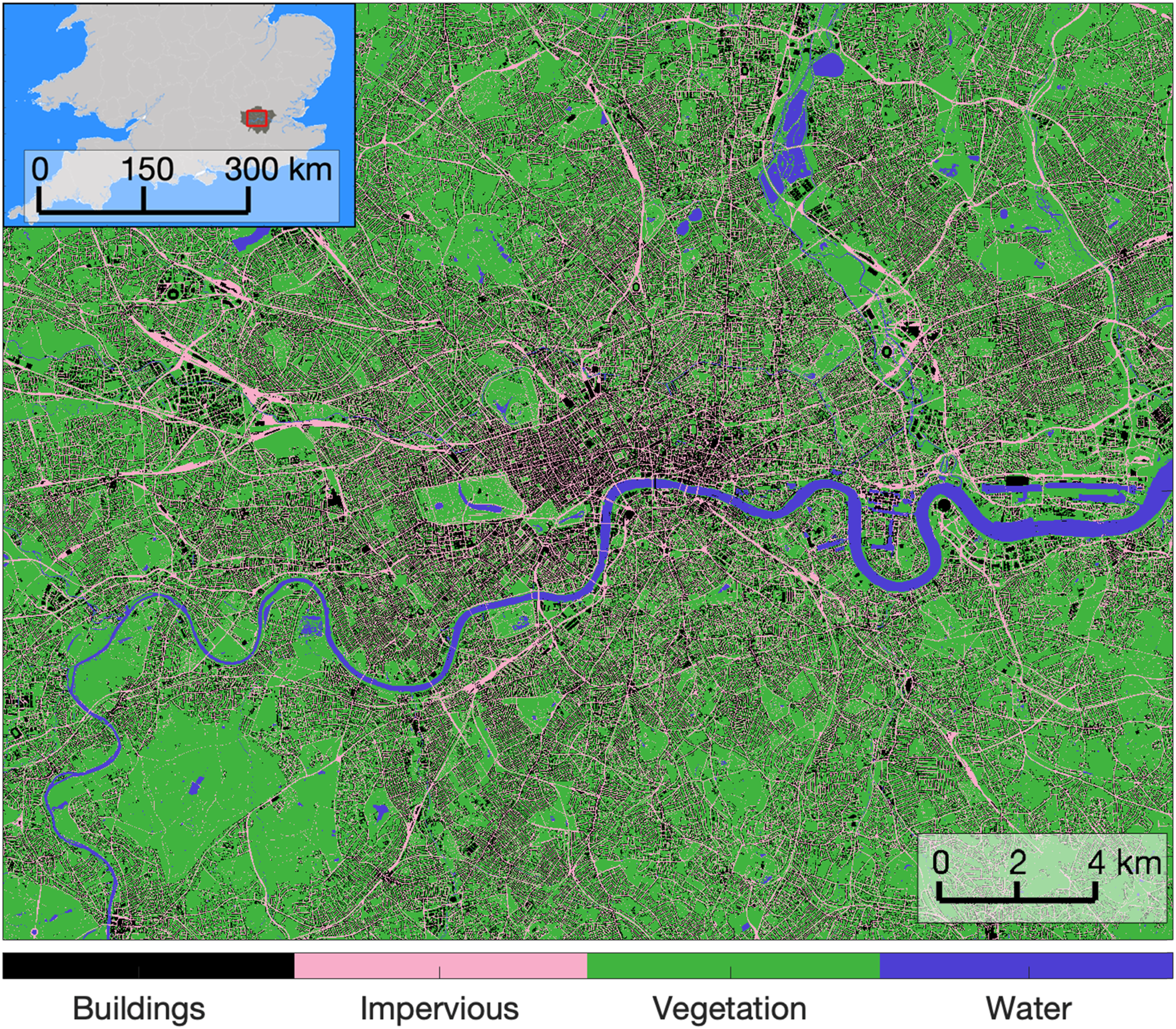

Morphometric indicators

We investigate different measurements of urban heterogeneity with the aim of providing useful additional information to models of surface-atmosphere interactions. As mentioned in the introduction, other than the basic physical representation, the heterogeneity indicators related to spatial configuration information of land types should be included to improve the urban surface representation in land-surface models. We employ several morphometric indicators to quantify the urban heterogeneity from compositional and configurational perspectives. The indicators selected must directly describe the structural heterogeneity, be present in multi-scale and measurable from data sources. The compositional heterogeneity with respect to different types of land-cover is quantified by the land-covers' plan area fractions and the evenness, and the frontal area index quantifies the compositional heterogeneity with respect to height. Contagion index and fractal dimensions of the land-cover types are used to characterise the configurational heterogeneity of the urban space in the aggregation/fragmentation and arrangement ways. The details of these morphometric indicators are described as below.

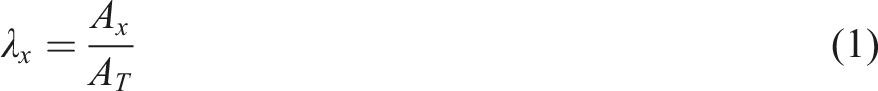
Plan area index

The plan area index of a land-cover type is expressed as (Oke et al., 2017)

λ_{x} = \frac{A_{x}}{A_{T}}

(1)

where the subscript

x

is the notation of land-cover type,

A_{x}

is the plan-view area occupied by the land-cover type, and

A_{T}

is the total ground surface area of interest. This study uses

λ_{b}

λ_{v}

λ_{i}

and

λ_{w}

to represent the plan area fractions of buildings, vegetation, impervious ground (roads, parking areas, etc.) and water cover, respectively. The plan area index relates to the density (or relative frequency) of the land-cover type, which is often an indication of the different functionalities of the urban space (greenspace, residential, commercial, etc.), reflecting urban planning and natural growth of cities.

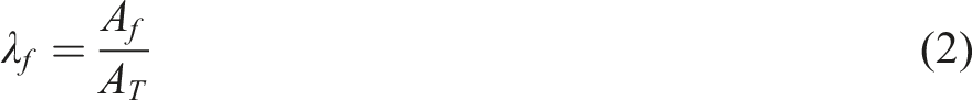
Frontal area index of buildings

The frontal area index indicates the wind-facing surface area of urban elements, which relates to the height of the elements and the “porosity” of the total urban environment. This parameter is relevant to the exchange of air and heat within the urban system, hence, to the mechanisms regulating the local urban climate. The frontal area index is given by

λ_{f} = \frac{A_{f}}{A_{T}}

(2)

where

A_{f}

is the total windward area of urban elements (Oke et al., 2017). This study considers only the windward area of buildings, where the windward area is defined as an average over all wind directions, employing the calculation method presented in Sützl et al. (2021b).

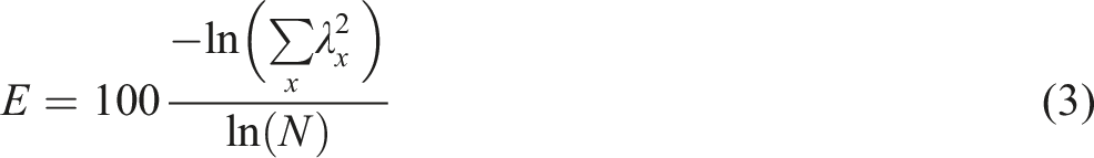
Evenness index

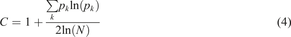
The evenness index characterizes the proportions of the different land-cover types. The expression of relative evenness is

E = 100 \frac{- \ln (\sum_{x} λ_{x}^{2})}{\ln (N)}

(3)

where

x

denotes the land-cover types (i.e.,

x = b, i, v, w

) and

N

is the number of land-cover types (Li and Reynolds, 1994; Romme, 1982). Evenness is a relative index with values between 0 and 100. When the area contains only one land-cover type,

E = 0

. When each land-cover type is equally present (i.e.,

λ_{x} = 1 / N

), then

E = 100

. In general, the greater the differences among proportions of land-cover types, the smaller

E

will be.

Contagion index

The contagion index describes the connectivity of land-cover types and granularity of the landscape texture by measuring the extent to which land-cover types are clumped together (Riitters et al., 1996). The adjacency state $k$ of a data pixel describes the combination of the land-cover type of the pixel itself and the land-cover type of an adjacent pixel. For a map with $N$ types of land-cover, the number of different adjacency states is therefore $N^{2}$ . Here we measure the adjacency state for the pixels below and to the right, respectively, yielding two adjacency states per pixel (Riitters et al., 1996). The contagion index is then given by (Li and Reynolds, 1993; Riitters et al., 1996)

C = 1 + \frac{\sum_{k} p_{k} \ln (p_{k})}{2 \ln (N)}

(4)

where

p_{k}

is the proportion of each adjacency state

k

in the total domain. Note that in equation (4) the summation is only performed over proportions

p_{k}

that are non-zero. The contagion index ranges from 0 to 1. A low contagion value indicates that the proportions of land-cover types and adjacency types are about the same, which may be related to a landscape with many small and highly dissected patches. A high contagion value can come from different proportions in land-cover types, or from one adjacency type being more frequent than the others, which can be same-type adjacency (i.e., clumping: large continuous patches of one land-cover type) or different-type adjacency (repeated spatial land-cover patterns) (Riitters et al., 1996; Wiese et al., 2021).

Fractal dimension

Fractals refer to geometries that cannot be described by regular shapes such as lines, squares, or cubes (Batty and Longley, 1994; Strogatz, 2018). Urban surface form resembles a fractal by considering the spatial distribution of an urban element (for example the buildings), which can be characterised by a fractal dimension (Batty and Longley, 1994). The fractal dimension measures the complexity and irregularity of fractals. As above, we use the land-cover types to define different fractals. This study uses the box counting method (Fernández and Jelinek, 2001) to calculate the fractal dimension $D_{x}$ which is performed by dividing the area up into squares of size $r_{m}$ , denoting the sum of all squares covering the elements of land-cover type $x = {b, i, v, w}$ as $F_{x, m}$ , and repeating this procedure for several $r_{m}$ . Since $F_{x, m}$ follows a powerlaw behaviour as $F_{x, m} \sim r_{m}^{D_{x}}$ , the fractal dimension $D_{x}$ is determined by applying linear regression between $\ln (F_{x, m})$ and $\ln (r_{m})$ (Chen et al., 2017; Chen and Huang, 2018; Sun and Southworth, 2013; Tannier and Pumain, 2005), since

\ln (F_{x, m}) = - D_{x} \ln (r_{m}) + c

(5)

where

c

is a constant. A fractal dimension of 0 indicates that the urban elements are at a single location. A fractal dimension of 1 indicates that the urban elements are spatially distributed along a line or simple curve. A fractal dimension of 2 indicates that the urban elements fill the two-dimensional space homogeneously. For urban surface form, the fractal dimension commonly lies between 1 and 2 (Batty and Longley, 1994).

Clustering algorithm

In order to explore heterogeneity on the city-scale, we use a clustering analysis of urban surface data on neighbourhood scale. The study area is divided into neighbourhood tiles of size 1 km × 1 km, which is similar to how urban surface data is processed for atmospheric models. The spatial properties of each tile are quantified using a vector of morphometric indicators introduced above. (hereafter referred to as a data point). The data are clustered using the $k$ -means algorithm (MacQueen, 1967), which aims to separate the data into $k$ groups, where each data point is assigned to the cluster that has the closest cluster mean. The optimal number of clusters is determined using the elbow method (Kodinariya and Makwana, 2013). This method performs the $k$ -means clustering for a sequence of numbers of clusters $k$ . The total within-cluster Euclidean distance $d (k)$ , as a function of $k$ , will decrease rapidly at a low number of clusters and decrease much slower after a certain value of $k$ , where there usually is a kink or elbow, and this value of $k$ is taken as the optimal number of clusters, so the elbow method determines the optimal number of clusters in a visual way. As the clustering results can be sensitive to the initial estimates of cluster centroids, we repeated the clustering 300 times and chose the result with the lowest total Euclidean distance, which ensures that the final cluster results are robust. To investigate whether the clustering results are sensitive to the chosen neighbourhood-scale or the way the domain is split up, the analysis was repeated also for neighbourhood tiles of sizes 0.5 km × 0.5 km and 2 km × 2 km, as well as a 1 km × 1 km domain shifted by 0.5 km in both the horizontal and vertical direction.

Results

Analysis of morphometric indicators

The spatial and frequency distributions of ten morphometric indicators at a resolution of 1 km are shown in Figure 2. The core of the city centre is densely covered by buildings accounting for about half of the land-cover, other areas have a lower building cover and average $λ_{b} = 0.2$ (Figure 2(a)). The plan area index of impervious ground $λ_{i}$ has a similar distribution to $λ_{b}$ with the exception that the core part does not stand out from the rest of the city centre (Figure 2(b)). On the contrary, greenspace covers only about 10-20% of the city centre, while it accounts for large proportion of the peripheric areas (Figure 2(c)). Notably, $λ_{v}$ has a much wider range of values than $λ_{b}$ and $λ_{i}$ , ranging from 0.1 to 1, which indicates that the spatial distribution of vegetation is highly heterogeneous over the study area. Most tiles contain few or no water, such that the irregular pattern of $λ_{w}$ highlights the river Thames and some larger local water bodies in the north of London (Figure 2(d)). The distribution of the frontal area index of buildings $λ_{f}$ is relatively similar to that of $λ_{b}$ , with the difference that $λ_{f}$ reaches much higher values in the core of the city centre, and thus has a larger spread of values overall (Figure 2(e)).

Figure 2.

Spatial and frequency distributions of ten morphometric indicators of Greater London at a resolution of 1 km: plan area indices of (a) buildings 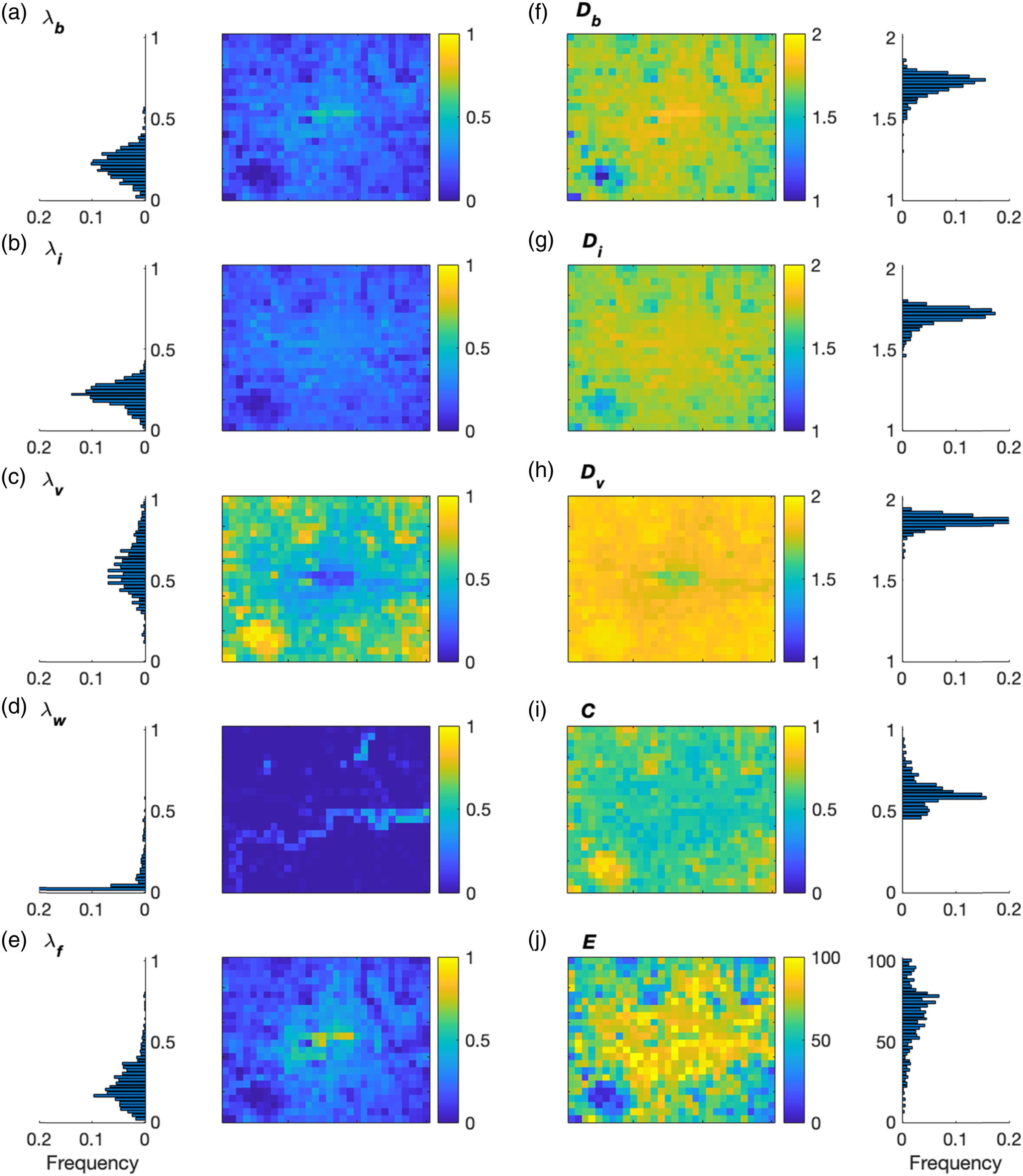$λ_{b}$ , (b) impervious surface $λ_{i}$ , (c) vegetation $λ_{v}$ , and (d) water $λ_{w}$ , (e) frontal area index of buildings $λ_{f}$ , fractal dimensions of (f) buildings $D_{b}$ , (g) impervious ground $D_{i}$ , and (h) vegetation $D_{v}$ , (i) contagion index $C$ , and (j) evenness index $E$ .

Spatial patterns between plan area index and fractal dimension of the same land-cover type are remarkably similar. This can be seen by looking at either end of the value spectrum: areas with a high plan area index $λ_{x}$ have a fractal dimension $D_{x}$ ( $x = {b, i, v}$ ) at the higher end of the value spectrum, and vice versa, suggesting that these two indicators are implicitly related. The fractal dimensions of buildings $D_{b}$ (Figure 2(f)) and impervious ground $D_{i}$ (Figure 2(g)), have a mean value of ∼1.7, while the average vegetation fractal dimension $D_{v} = 1.9$ (Figure 2(h)). This means that particularly vegetation fills the domain relatively uniformly, presumably through the abundance of small-scale elements such as street trees. Note that the fractal dimension cannot be computed when the land-cover type is absent. Since this leaves the fractal dimension for water $D_{w}$ undefined for many tiles, $D_{w}$ was omitted here.

For the extent of aggregation of land-cover, most areas show weak connectivity of one land-cover type, with a contagion index $C$ between 0.5 and 0.7, except for where vegetation cover is large and contiguous, yielding a contagion index of almost 1 (Figure 2(i)). The spatial pattern of evenness $E$ is the most diverse since its range has the widest spread (Figure 2(j)). In contrast to contagion, evenness has high values in the centre of London, since the proportions of land-cover types in these areas are relatively uniformly distributed, while low values are observed in peripheral areas with abundant vegetation, i.e., a large proportion of a single land-cover type.

Comparison of the spatial patterns of the morphometric indicators suggests that there is redundant information between these ten indicators. To assess the overlap of information, correlation coefficients between the morphometric indicators are calculated and summarised in Table 1. Figure 3 shows the tile-wise correlations for some of the indicators with the highest correlation coefficients. Plan area index

λ_{x}

and fractal dimension

D_{x}

for the same land-cover type (

x = {b, i, v}

) are strongly positively correlated (Figure 3(a)-(c)). If the plan area index is low, it is unlikely that that land-cover type is distributed homogeneously across the neighbourhood tile, and therefore

D_{x}

is at the lower value range. Conversely, if the plan area index is high, the land-cover type is more likely to be spread out across the entire tile, which yields a fractal dimension closer to 2. Evenness and contagion show a strongly negative correlation (Figure 3(d)), as previously noted by Li and Reynolds (1994). This suggests that landscapes with uniform proportions of land cover tend to have many dissected, randomly distributed patches rather than having each type clumped together individually. Moreover,

λ_{b}

is positively correlated with

λ_{f}

(Figure 3(e)), and negatively correlated with

λ_{v}

(Figure 3(f)). This result is expected, because urbanization means the decrease of natural greenspace, and both

λ_{b}

and

λ_{f}

are associated with the built environment. However, in contrast to the indicators discussed previously, the relation between

λ_{b}

and

λ_{f}

, and between

λ_{b}

and

λ_{v}

, is not one-to-one (Figure 3(e)-(f)).

Table 1.

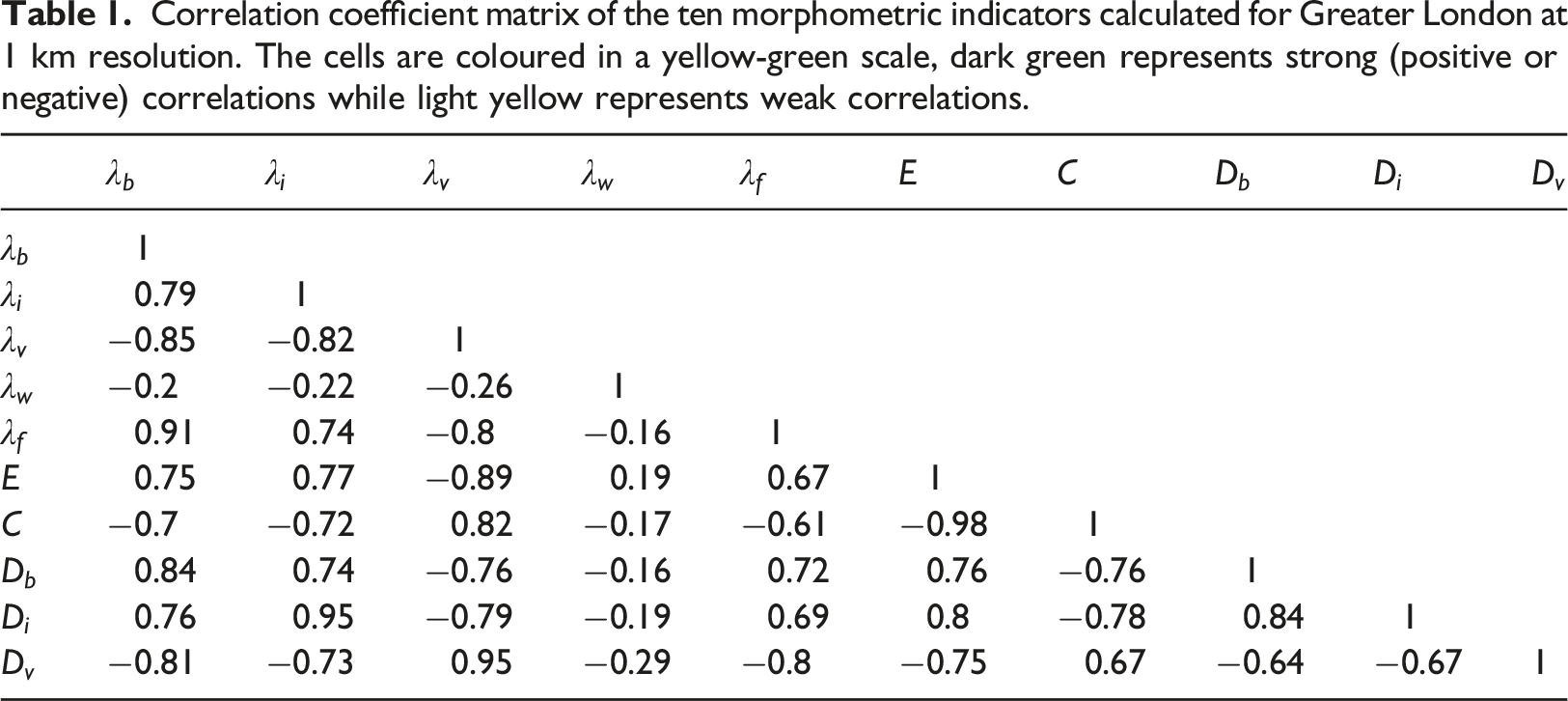
Correlation coefficient matrix of the ten morphometric indicators calculated for Greater London at 1 km resolution. The cells are coloured in a yellow-green scale, dark green represents strong (positive or negative) correlations while light yellow represents weak correlations.

	$λ_{b}$	$λ_{i}$	$λ_{v}$	$λ_{w}$	$λ_{f}$	$E$	$C$	$D_{b}$	$D_{i}$	$D_{v}$
$λ_{b}$	1
$λ_{i}$	0.79	1
$λ_{v}$	−0.85	−0.82	1
$λ_{w}$	−0.2	−0.22	−0.26	1
$λ_{f}$	0.91	0.74	−0.8	−0.16	1
$E$	0.75	0.77	−0.89	0.19	0.67	1
$C$	−0.7	−0.72	0.82	−0.17	−0.61	−0.98	1
$D_{b}$	0.84	0.74	−0.76	−0.16	0.72	0.76	−0.76	1
$D_{i}$	0.76	0.95	−0.79	−0.19	0.69	0.8	−0.78	0.84	1
$D_{v}$	−0.81	−0.73	0.95	−0.29	−0.8	−0.75	0.67	−0.64	−0.67	1

Figure 3.

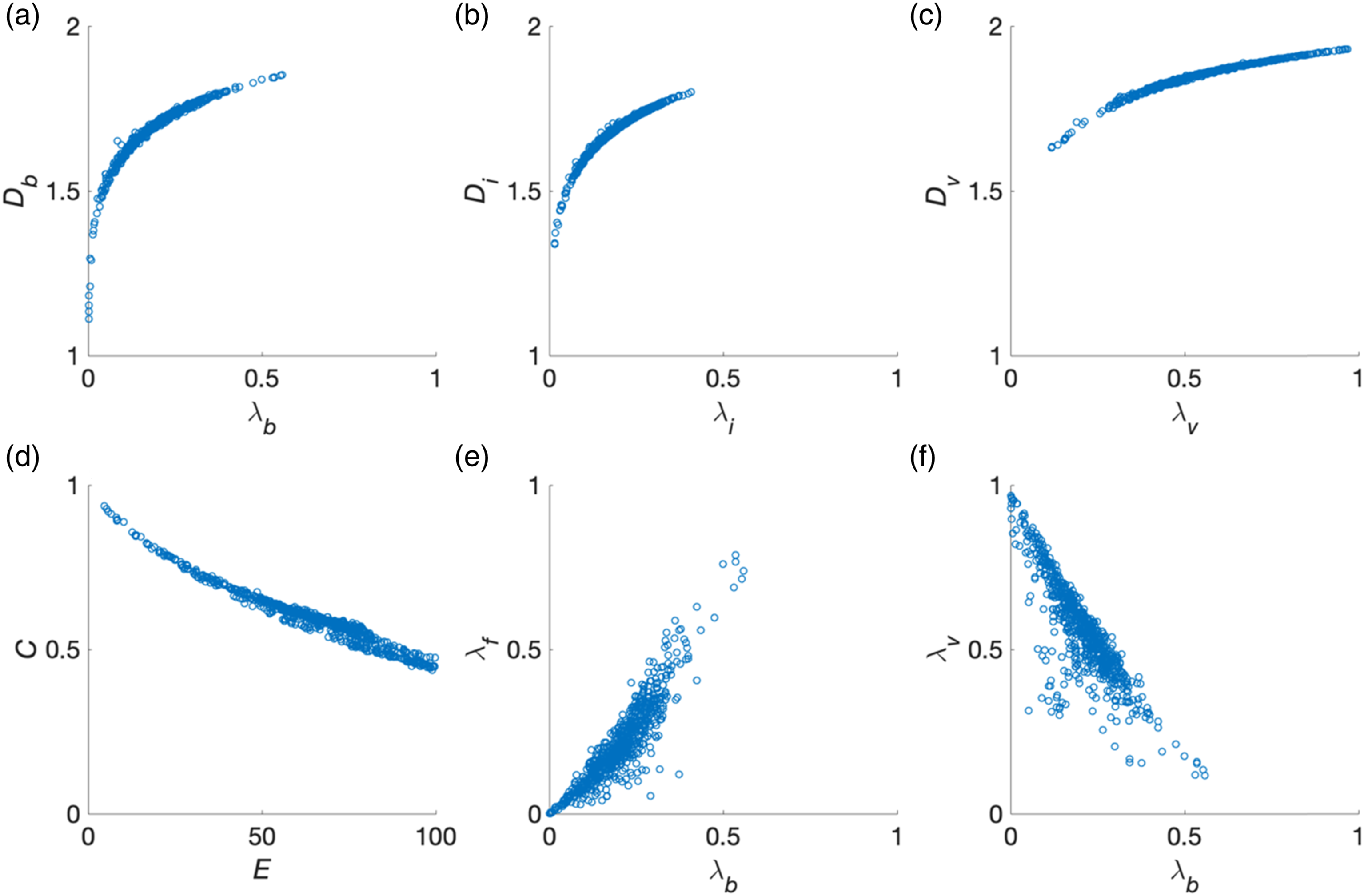
Pairwise correlations between plan area indices and fractal dimensions of (a) buildings, (b) impervious surface, and (c) vegetation, between (d) evenness and contagion, (e) plan area index and frontal area index of buildings, and (f) plan area indices of buildings and vegetation for each 1km²-tile in Greater London.

In the clustering analysis that follows, we will therefore discard the fractal dimension and the evenness indicators, as these are well represented by other indicators. We choose contagion over evenness because the correlation between contagion and the plan area indices is weaker than that between evenness and the plan area indices. Then, the remaining six indicators include the plan area indices of four land-cover types, the frontal area index of buildings, and contagion.

Clustering analysis

A $k$ -means clustering algorithm is applied to classify neighbourhood types based on the reduced set of six heterogeneity indicators at 1 km × 1 km grid resolution. The elbow method suggests that the optimal number of clusters is six (Figure S1). The resulting neighbourhood classification map of Greater London is displayed in Figure 4. The typical urban morphologies in each neighbourhood type were identified using the morphometric indicators only, but Figure 4 clearly shows that the clustering also distinguishes categories of urban function, by separating Greater London into zones with distinct functional properties. The six neighbourhood types can be associated with greenspace (GS), water (W), sparse sub-urban areas (SSU), compact sub-urban areas (CSU), mixed-type residential and commercial zones (MTR) and central business districts (CBD), respectively.

Figure 4.

Classification map of the study area into six neighbourhood types: greenspace (GS), water (W), sparse sub-urban (SSU), compact sub-urban (CSU), mixed-type residential (MTR), and central business district (CBD). The sample tile discussed in the hierarchical decomposition is outlined in black.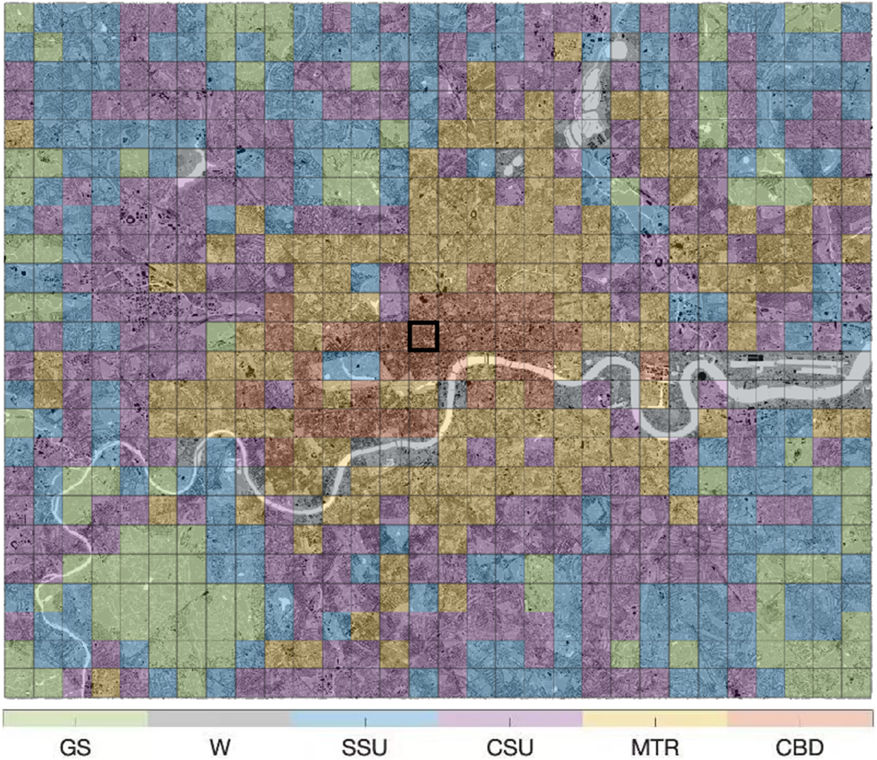

Since the morphometric indicators take values from a continuous distribution (cf. Figure 2) rather than a discrete set of values, the morphometric indicators cover a range of values within each cluster and can also partially overlap between clusters (Figure S2). To identify whether the clustering results are subject to a modifiable-areal-unit-problem (MAUP) bias, the full analysis was repeated for three other cases: two different grid resolutions (0.5 and 2 km) and a modified study domain (shifted by 0.5 km). The maps for different resolutions and shifted neighbourhoods are largely the same (Figure S3), and the elbow method also indicate that 6 clusters are optimal except for the 2 km resolution, which shows that 5 is the optimal number of categories (Figure S1). Inspection shows that the central business district cluster disappears in the 2 km case. This can be understood by realizing that these are often high-rise clusters which tend to be smaller than 2 $\times$ 2 km². This investigation suggests that the results of the neighbourhood-scale clustering are not MAUP-biased. The sensitivity check of the clustering algorithm with different initial conditions confirmed that, by choosing the clustering result with the lowest Euclidian distance, we produce a robust clustering: 1) the within-cluster distance of the 300 runs generally does not vary by more than 2%; and 2) repeating of the full clustering analysis (i.e. 300 runs) with different initial conditions produces virtually identical clusters (<0.5% difference). The remaining analysis will focus on the neighbourhood classification of the 1 km × 1 km base case.

The average value and range of the morphometric indicators within each neighbourhood type for the base case are summarised in Table 2. Example tiles for each neighbourhood type are shown in Figure 5, and the main urban features for each neighbourhood type are described below.

Table 2.

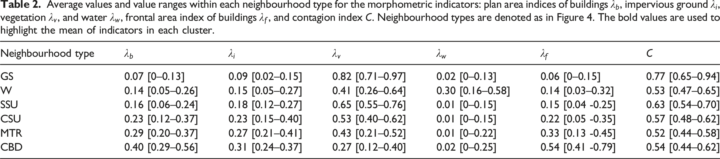
Average values and value ranges within each neighbourhood type for the morphometric indicators: plan area indices of buildings $λ_{b}$ , impervious ground $λ_{i}$ , vegetation $λ_{v}$ , and water $λ_{w}$ , frontal area index of buildings $λ_{f}$ , and contagion index $C$ . Neighbourhood types are denoted as in Figure 4. The bold values are used to highlight the mean of indicators in each cluster.

Neighbourhood type	$λ_{b}$	$λ_{i}$	$λ_{v}$	$λ_{w}$	$λ_{f}$	C
GS	0.07 [0–0.13]	0.09 [0.02–0.15]	0.82 [0.71–0.97]	0.02 [0–0.13]	0.06 [0–0.15]	0.77 [0.65–0.94]
W	0.14 [0.05–0.26]	0.15 [0.05–0.27]	0.41 [0.26–0.64]	0.30 [0.16–0.58]	0.14 [0.03–0.32]	0.53 [0.47–0.65]
SSU	0.16 [0.06–0.24]	0.18 [0.12–0.27]	0.65 [0.55–0.76]	0.01 [0–0.15]	0.15 [0.04 -0.25]	0.63 [0.54–0.70]
CSU	0.23 [0.12–0.37]	0.23 [0.15–0.40]	0.53 [0.40–0.62]	0.01 [0–0.15]	0.22 [0.05 -0.35]	0.57 [0.48–0.62]
MTR	0.29 [0.20–0.37]	0.27 [0.21–0.41]	0.43 [0.21–0.52]	0.01 [0–0.22]	0.33 [0.13 -0.45]	0.52 [0.44–0.58]
CBD	0.40 [0.29–0.56]	0.31 [0.24–0.37]	0.27 [0.12–0.40]	0.02 [0–0.25]	0.54 [0.41 -0.79]	0.54 [0.44–0.62]

Figure 5.

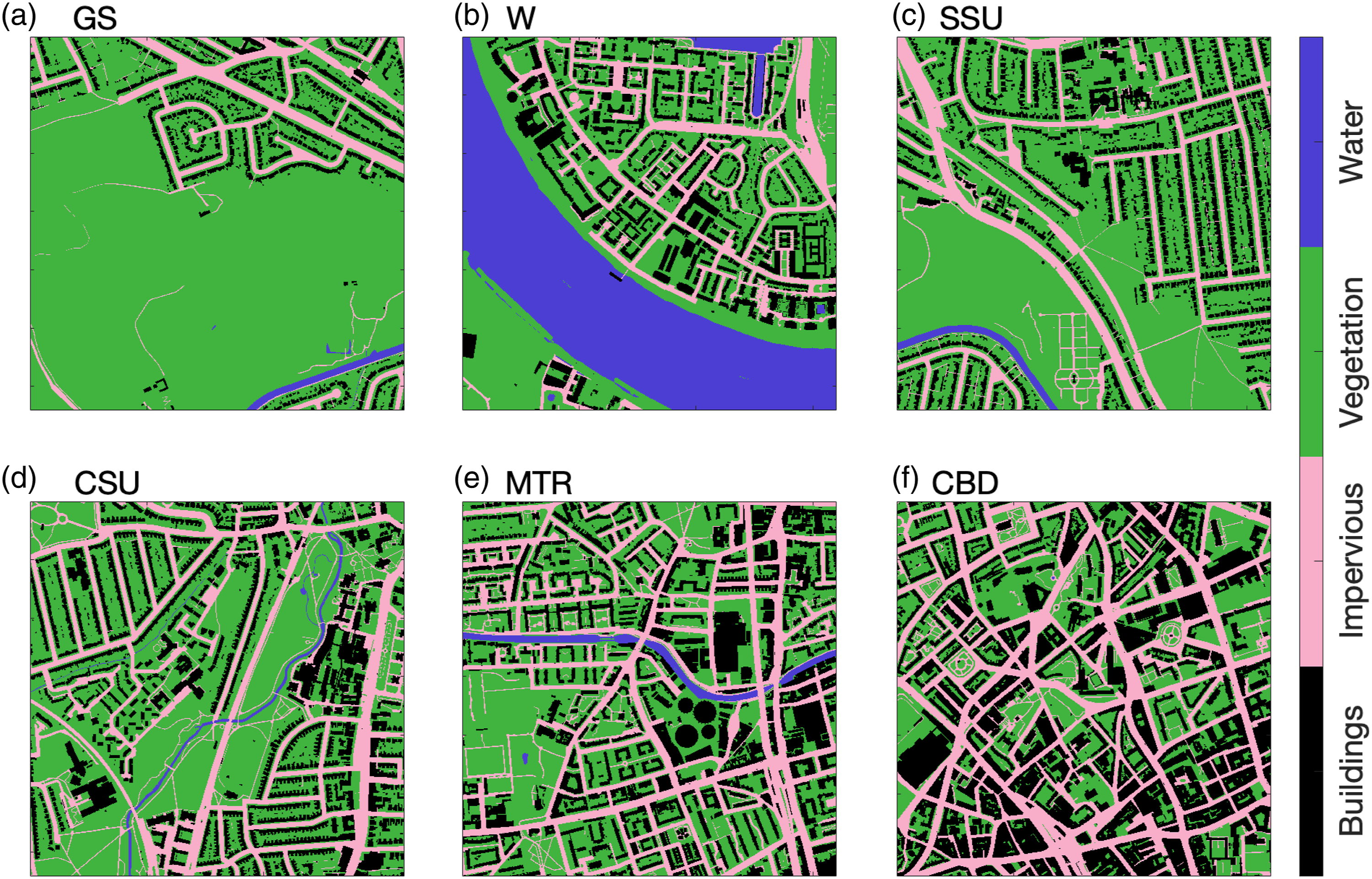
Example tiles for (a) greenspace (GS), (b) water (W), (c) sparse sub-urban (SSU), (d) compact sub-urban (CSU), (e) mixed-type residential (MTR), and (f) central business district (CBD).

Greenspace (GS) is predominantly covered by vegetation with an average plan area index of $λ_{v} = 0.82$ . A few small-sized cottages are located along the roads. The composition of land-cover types is highly non-uniform, and the spatial arrangement with a large and continuous vegetation cover yields the maximum contagion index among the six neighbourhood types (average $C = 0.77$ ). Tiles in GS are mainly located in the periphery of the study area and are associated with large parks or nature reserves.

Water (W) is the only neighbourhood type with a significant water coverage of $λ_{w} = 0.3$ . The most notable feature is the river Thames passing through central London and large water reservoirs in the north. Water covers on average about twice as much area as buildings (average $λ_{b} = 0.14$ ) or impervious surface (average $λ_{i} = 0.15$ ). The similar proportions of buildings and impervious surface and similar proportions of vegetation and water increase the uniformity degree of composition, yielding the second smallest value for contagion.

Sparse sub-urban areas (SSU) are characterised by a low density of mainly low-rise, single-family buildings (average $λ_{b} = 0.16$ ) along residential streets surrounded by contiguous greenspace (average $λ_{v} = 0.65$ ). The average contagion index is the second highest amongst the neighbourhood types ( $C = 0.63$ ), which is likely related to the large and contiguous vegetation cover and repeated spatial patterns of sub-urban residential areas with rows of houses lined up along the roads, each with their vegetated backyards (cf. Figure 5(c)).

Compact sub-urban areas (CSU) have a lower proportion of vegetation (average $λ_{v} = 0.53$ ) and more compact buildings and impervious surface (average $λ_{b}, λ_{i} = 0.23$ ) compared with the sparse sub-urban zones, containing also mid-rise buildings like schools or hospitals. The spatial arrangement of buildings and roads appears relatively similar to SSU, but also shows larger clusters of built infrastructure, e.g., around local train stations. The more equal distribution of land cover compared to SSU reduces the compositional heterogeneity and increases the land-cover fragmentation, which yields a lower contagion index than SSU. The CSU has the largest number of tiles accounting for about one third of the whole study area. It could reflect the medium level of urbanization.

The mixed-type residential zone (MTR) represents a higher level of urbanization with residential, commercial, and industrial areas. Residential houses are either compact low-rise buildings with little greenspace, or open mid- to high-rise buildings surrounded by green areas. In MTR, the built-up and impervious surface cover exceed the pervious surface cover (vegetation, water). The average contagion index is the lowest amongst the neighbourhood types ( $C = 0.52$ ) since the landscape is fragmented into many small patches.

Central business district (CBD) is a highly developed and urbanized region in Greater London, characterised by compact arrangement of buildings, a few sporadic greenspaces and complex transport networks. The occurrence of many mid-rise and high-rise buildings is shown by the average frontal area index $λ_{f} = 0.54$ , which is significantly larger than the building plan area index (average $λ_{b} = 0.4$ ). In other five neighbourhood types, these two values are almost identical. The tall buildings are closely spaced by staggered roads, forming many street canyons with narrow widths. The landscape in CBD is divided into many small and highly dissected fragments, resulting in a low contagion index.

The different neighbourhood type (with exception of the water cluster) can also be distinguished by the proximity to the city centre: GS, SSU, CSU, MTR, and CBD (GS being furthest away and CBD being closest). Buildings, impervious surface, and frontal area indices increase as the distance from city centre decreases, implying urbanization is accompanied by the increased need to transport people and goods, while vegetation cover decreases. In addition, urbanization tends to increase the composition uniformity but promotes land fragmentation, which yields a decreasing contagion index with higher urbanization.

It is interesting to investigate how the detected neighbourhood types identified here compare to Local Climate Zones (LCZs, Stewart and Oke, 2012), which describe distinct categories of urban areas in terms of the land cover type, the height and compactness of buildings and vegetation. Each LCZ is associated with a specific range of morphology indicators (see Stewart and Oke (2012) for details). Below we determine the LCZ(s) associated with each neighbourhood type using those indicators available as within-cluster means (Table 2).

Both CSU and MTR correspond to LCZ 6 (open low-rise), and CBD corresponds to LCZ 3 (compact low-rise; see Table S2). Neither GS, W, nor SSU have a direct LCZ correspondence. These associations also change with resolution: while there are more correspondences of neighbourhood types with LCZs at 0.5 km resolution, there are almost none at 2 km (Table S2), and some mappings change with the shifted grid. We find that there is no one-to-one correspondence between the identified neighbourhood types and LCZ classes, and that the mapping between them is not robust. Mouzourides et al. (2019) similarly found that LCZ maps derived from morphometric indicators can be resolution dependent: they found 16 different LCZs in Greater London at a resolution of 100 m × 100 m, whereas at a resolution of 1.6 km × 1.6 km, the number of classes reduced to 6.

Hierarchical decomposition

In this section we explore heterogeneity within the 1 $\times$ 1 km² neighbourhood-scale tiles by considering the properties of each neighbourhood type at a range of different measurement scales. Indeed, heterogeneity is dependent on the measurement scale, meaning that urban surface properties which are heterogeneous will become homogeneous as the measurement scale increases (Cullinan and Thomas, 1992; Li and Reynolds, 1995; Murwira, 2003; Oke et al., 2017). The approach is based on repeated coarse-graining: starting from an original map $I_{M}$ with resolution of $2^{M} \times 2^{M}$ pixels, each coarse-graining operation reduces the resolution in each direction by a factor two, as shown in Figure 6. We will denote the coarse-grained maps $I_{m}$ where $m < M$ . When $m = M$ it represents the original map, when $m = M - 1$ , the map is coarse-grained once, when $m = M - 2$ twice and so on. More specifically, $I_{m}$ contains $2^{m} \times 2^{m}$ pixels, implying that each of its pixels represents the information of $2^{M - m} \times 2^{M - m}$ pixels of $I_{M}$ . The associated length scale is $r_{m} = 1000 / 2^{m}$ m. We will first explore the properties of the coarse-grained maps, and then introduce a hierarchical decomposition map $J_{m}$ , which represents the difference between the maps at resolution $m$ and $m - 1$ (defined rigorously below). The aim of this analysis is to quantify what happens to morphometric indicators upon changing the resolution, at what resolution the changes are largest and to quantify heterogeneity across multiple scales. It is hoped that this information ultimately will be of use in quantifying the effects of changing resolution in land-surface model predictions. The method presented here is closely related to Multi-Resolution Analysis (MRA) and wavelets (Mouzourides et al., 2013, 2014).

Figure 6.

Example of coarse-grained and hierarchical maps for 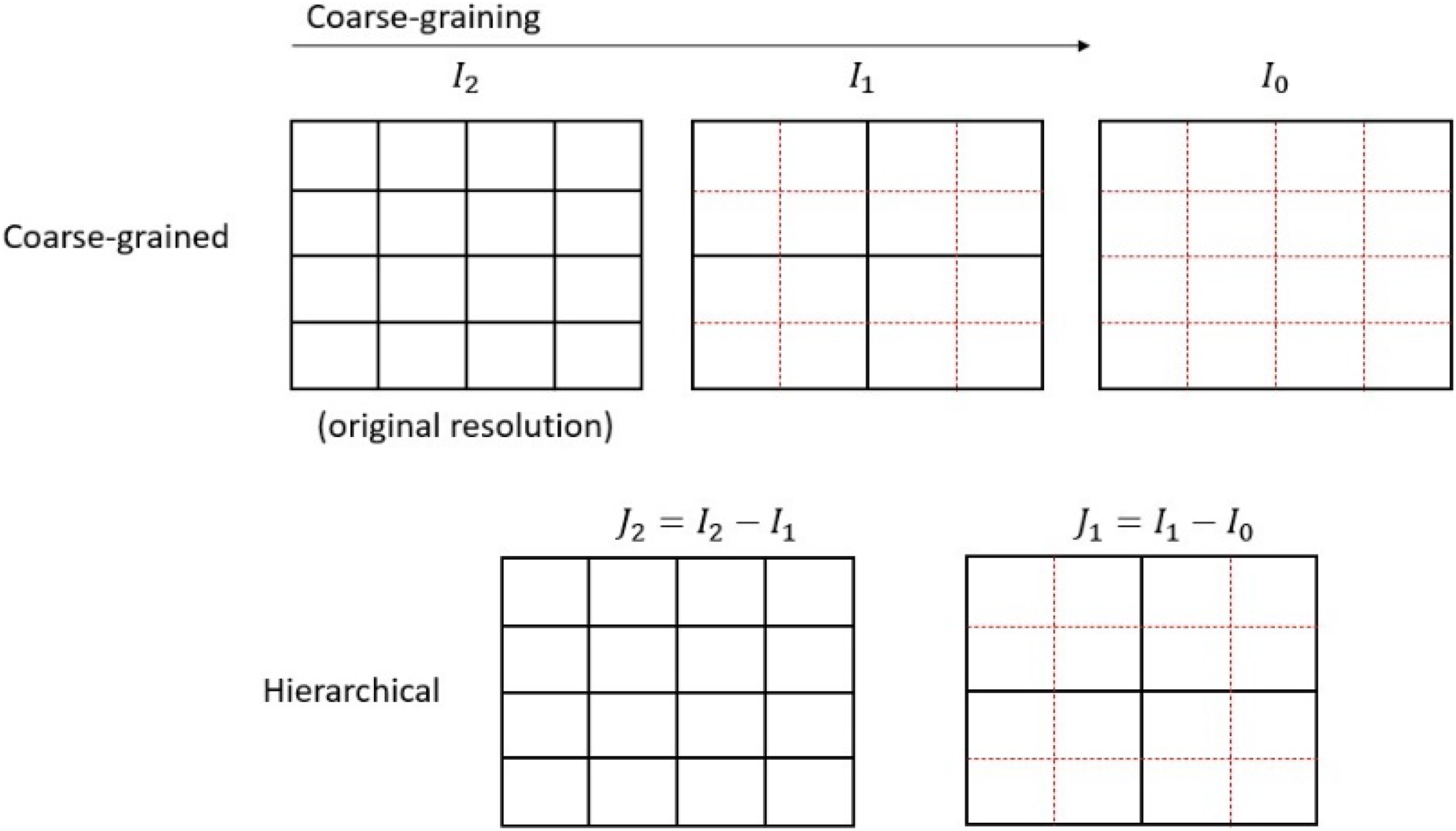$M = 2$ . Map $I_{2}$ is the original map containing $2^{M} \times 2^{M}$ pixels which can be coarse-grained twice (maps $I_{1}$ and $I_{0}$ ). The hierarchical maps are obtained by taking the difference between two neighbouring coarse-grained maps.

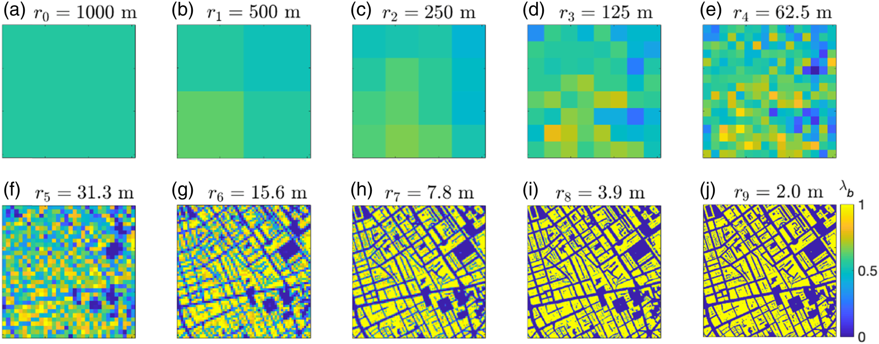
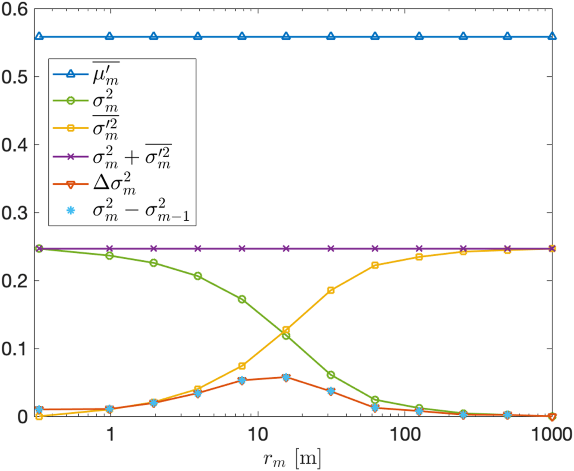
The resolution of the neighbourhood tiles is 3200 $\times$ 3200 which is not a power of two, therefore some interpolation is necessary before the analysis can be conducted. To have as many exact divisions by a factor of two as possible, the tiles were interpolated using a nearest-pixel approach to 3072 $\times$ 3072 pixels at 0.3255 m resolution. Since 3072 = 3 $\times$ 2¹⁰, this allows the maps to be divided by a factor of two for 10 times, and finally scaled down by a factor three to obtain the finest resolution (pixel-based) raster map. This refinement gives in total twelve levels of resolution ( $m$ ranging from 0 to $M = 11$ ). Figure 7 shows the first ten maps $I_{m}$ of $λ_{b}$ for a sample tile outlined in Figure 4 at the computed length scales $r_{m}$ .

Figure 7.

Maps $I_{m}$ of building plan area index $λ_{b}$ at measurement scales $r_{m}$ of (a) 1000 m, (b) 500 m, (c) 250 m, (d) 125 m, (e) 62.5 m, (f) 31.3 m, (g) 15.6 m, (h) 7.8 m, (i) 3.9 m, and (j) 2 m. The location of the selected area is outlined in Figure 4.

To quantify the statistical properties of each map $I_{m} (i, j)$ , we introduce the following notation: the tile-based mean at resolution level $m$ is $μ_{m}$ , and the tile-based variance (i.e., the variance between the cells, or resolved variance) is denoted by $σ_{m}^{2}$ . These quantities (the resolved statistics) can be directly computed from the maps $I_{m}$ (cf. Figure 6). For each cell in $I_{m} (i, j)$ , we denote the within-cell mean and variance at resolution level $m$ as $μ_{m}^{'} (i, j)$ and $σ_{m}^{'^{2}} (i, j)$ . In Figure 7, the within-cell mean values $μ_{m}^{'} (i, j)$ simply correspond to the $λ_{b}$ values shown: i.e., $I_{m} (i, j) \equiv μ_{m}^{'} (i, j)$ . The within-cell variance is a result of the coarse-graining process at length scale $r_{m}$ and is calculated from the input map (i.e. $I_{M}$ ). The average of the cell-based values over the entire tile will be denoted with an overbar: ${\bar{μ^{'}}}_{m}$ for the tile-averaged within-cell mean, and $\bar{σ_{m}^{'^{2}}}$ for the tile-averaged within-cell variance. These quantities are related to the tile-based statistical quantities of the original (pixel-based) map $I_{M}$ as

\forall m \in [0, M] : {\bar{μ^{'}}}_{m} = μ_{M},

(6)

σ_{m}^{2} + \bar{σ_{m}^{'^{2}}} = σ_{M}^{2},

(7)

which follows from the linearity of the mean and the variance decomposition formula (also called law of total variance; Pishro-Nik, 2014). Equation (6) states that the mean over the entire tile is conserved across various resolutions. Equation (7) states that the variance in the tile is conserved as the sum of the between-cell variance and the averaged within-cell variance. Figure 8 depicts the statistical properties of the maps

I_{m}

from Figure 7 as functions of the measurement scale

r_{m}

. As expected from the equations above, the between-cell variance

σ_{m}^{2}

and averaged within-cell variance

\bar{σ_{m}^{'^{2}}}

vary oppositely with

r_{m}

: as the measurement length

r_{m}

increases, the resolved contribution

σ_{m}^{2}

will reduce while the within-cell contribution

\bar{σ_{m}^{'^{2}}}

increases.

Figure 8.

Statistics of the sample tile (Figure 7) and its hierarchical decomposition against length scale $r_{m}$ . The statistical quantities are: tile-averaged within-cell mean ${\bar{μ^{'}}}_{m}$ , between-cell variance $σ_{m}^{2}$ , tile-averaged within-cell variance $\bar{σ_{m}^{'^{2}}}$ , and scale variance $Δ σ_{m}^{2}$ . Note that the measurement scale $r_{m}$ is logarithmic.

We introduce a hierarchical decomposition of the data that helps to explore the heterogeneity present at different resolutions of 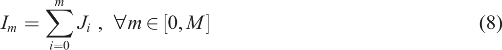$I_{m}$ . The decomposition at resolution level $m$ is based on the difference between two successive maps $J_{m} = I_{m} - I_{m - 1}$ . Setting $J_{0} = I_{0}$ , this implies that the map $I_{m}$ can be computed as the sum of decomposition maps $J_{m}$ as

I_{m} = \sum_{i = 0}^{m} J_{i}, \forall m \in [0, M]

(8)

Figure 9 displays the decomposition maps $J_{m}$ at various resolutions, clearly outlining the “corrections” that are needed to move from resolution level $m - 1$ to level $m$ . This hierarchical decomposition shares some features with Fourier decomposition in that it breaks up an image into features at particular scales but has two important differences: 1) there is not a single amplitude/phase linked to a particular scale; and 2) the hierarchical decomposition is intrinsically local – if there are areas that are uniform above resolution level $m$ , then the corrections will be zero for higher level maps. This is clearly seen in Figure 9, where parks (i.e., a larger area without buildings) become visible as white spots around $r_{m} = 15.6$ m (Figure 9(g)), and these locations remain unchanged at higher resolutions.

Figure 9.

Hierarchical decomposition maps 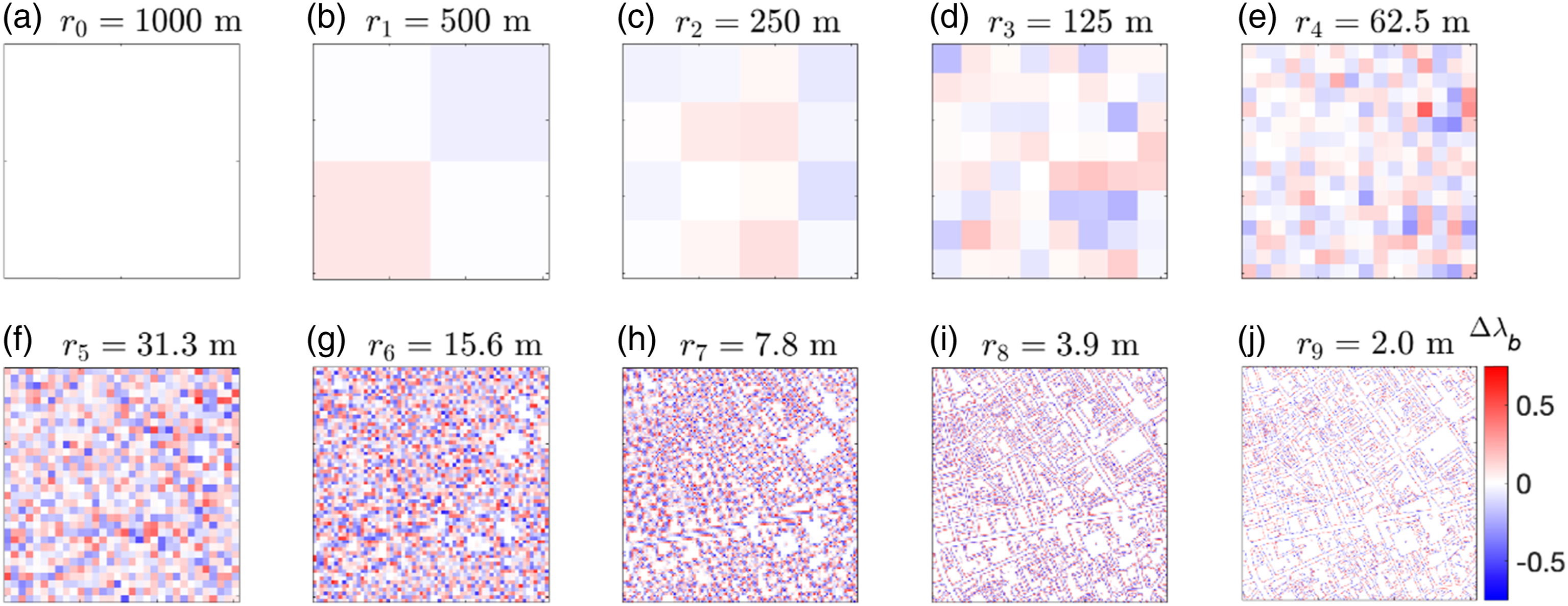$J_{m}$ of plan-area index $λ_{b}$ of the sample tile (Figure 7) at measurement scales $r_{m}$ of (a) 1000 m, (b) 500 m, (c) 250 m, (d) 125 m, (e) 62.5 m, (f) 31.3 m, (g) 15.6 m, (h) 7.8 m, (i) 3.9 m, and (j) 2 m.

An attractive feature of the hierarchical decomposition is that the tile-based variance of a map $J_{m}$ , which we refer to as scale variance and denote by $Δ σ_{m}^{2},$ can be shown to directly link the resolved variances in the maps $I_{m - 1}$ and $I_{m}$ as $Δ σ_{m}^{2} = σ_{m}^{2} - σ_{m - 1}^{2}$ (see the overlapping lines of $Δ σ_{m}^{2}$ and $σ_{m}^{2} - σ_{m - 1}^{2}$ in Figure 8). Therefore, the hierarchical decomposition distributes the variance into its contribution at different scales. This implies that $Δ σ_{m}^{2}$ represents the proportion of within-cell variance that becomes resolved by doubling the resolution. This allows for the interpretation of the scale variance $Δ σ_{m}^{2}$ as an “energy spectrum”, which is often used for identification of the energetic scales in multi-scale problems (Pope, 2000). Figure 8 shows the scale variance $Δ σ_{m}^{2}$ as a function of the measurement scale $r_{m}$ , which can be seen to peak around 15.6 m, implying that this is the dominant (or most energetic) length scale. This length scale is also roughly where the between-cell and averaged within-cell variances cross over.

Below we conduct an analysis for the multi-scale properties of the neighbourhood types identified in the clustering analysis using the hierarchical decomposition described above. Hierarchical maps $J_{m}$ of the four plan area indices $λ_{b}, λ_{i}, λ_{v},$ and $λ_{w}$ are constructed for each tile in the study area. These resulting tile-based statistics are then further averaged over all tiles within the cluster to identify the differences between the neighbourhood types. Figure 10(a)-(d) shows the cluster averages of the scale variance $Δ σ_{m}^{2}$ for each land-cover type.

Figure 10.

Cluster-averaged scale variance 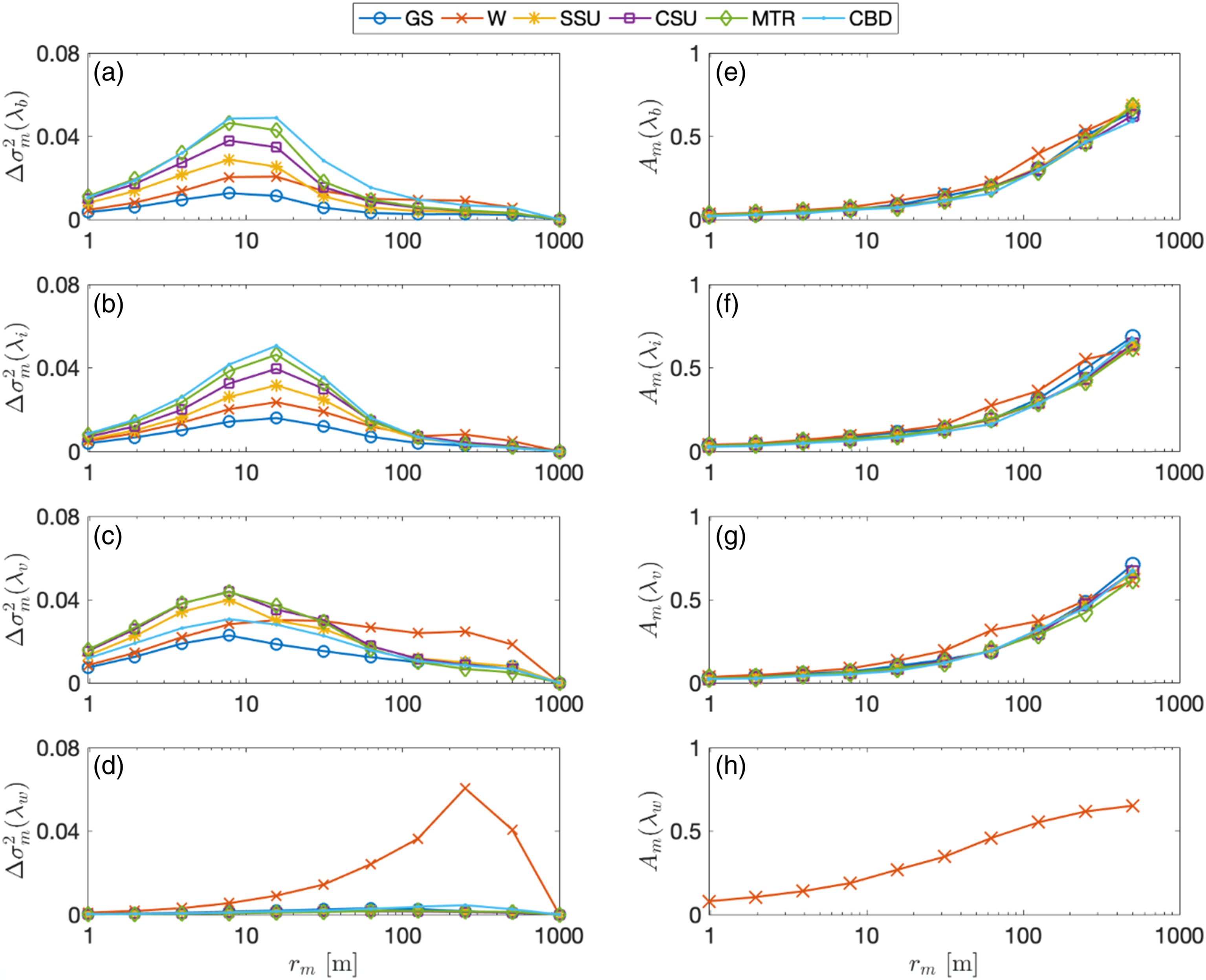$Δ σ_{m}^{2}$ and anisotropies $A_{m}$ for plan-area indices of (a, e) buildings $λ_{b}$ , (b, f) impervious ground $λ_{i}$ , (c, g) vegetation $λ_{v}$ , and (d, h) water $λ_{w}$ at different scales. Note that the measurement scale $r_{m}$ is logarithmic.

For building cover,the cluster-averaged scale variance $Δ σ_{m}^{2} (λ_{b})$ (Figure 10(a)) increases with measurement scale $r_{m},$ peaks at 7.8 m or 15.6 m and subsequently decreases with measurement scale. This distribution is similar for all neighbourhood types, where a higher average building plan area index is accompanied by larger variance. The observation that the maximum scale variance occurs at 7.8 m or 15.6 m implies that these two scales contribute most to the total variance of the neighbourhoods, and equivalently that these scales represent the dominant lengths at which individual building becomes resolved. For example, the individual building in Figure 7, classified into CBD, start to be resolved at a scale of 15.6 m (Figure 7(g)). For scales smaller than 15.6 m, there are almost no changes in $λ_{b}$ (cf. Figure 7(h)-(j)), and small changes primarily concern the boundaries of the buildings, as indicated by the hierarchical decomposition in Figure 9(h)-(j). For scales between 15.6 m and 62.5 m, several buildings begin to blur into a single cell, leading to a significant variance in $λ_{b}$ (cf. Figure 7(e)-(f) and Figure 9(e)-(f)). As the scale increases, the averaging procedure covers more buildings by a single cell, resulting in relatively less change of $λ_{b}$ at each level.

The scale variance of impervious ground (Figure 10(b)) exhibits a similar distribution for all neighbourhood types across the length scales with a clear maximum at a scale of 15.6 m, which is a width typical for a road. Similar to the building cover, the magnitude of the scale variance is linked to the magnitude of the plan area index, where $Δ σ_{m}^{2} (λ_{i})$ is highest for the CBD that meanwhile has the highest average values for $λ_{b}$ and $λ_{i}$ , suggesting that each increase in resolution results in larger changes than in the other neighbourhood types, and the “gains” from increasing the resolution are therefore highest for these urban neighbourhoods.

The scale variance of vegetation has a similar distribution for each neighbourhood type with a peak at a scale of 7.8 m, with the exception of the water neighbourhood type, in which the scale variance is nearly uniformly distributed across most length scales, suggesting that there is no dominant length scale for vegetation in the water neighbourhood type (Figure 10(c)). The peak at the maximum variance at scale 7.8 m is weaker compared to the peaks in building and impervious cover, and the relation between higher variances and higher (vegetation) land-cover is not always maintained. A typical length scale for vegetation is therefore not obvious from the data. The greenspace cluster shows least variance and a weak dependence on scale, suggesting that the tiles identified in GS indeed primarily consist of large green spaces and therefore, small changes are required upon moving to higher resolutions.

All neighbourhood types except for the water cluster contain almost no water (averaged $λ_{w} \leq 0.02$ ) and therefore have very low scale variance at all resolutions, which implies that there is no strong dominant length scale for water in these neighbourhood types (Figure 10(d)). The water neighbourhood type, however, displays a strong peak at 250 m, implying that tiles in this type are dominated by water (averaged $λ_{w} = 0.3$ ) in form of a large contiguous body of water with dominant width around 250 m. Clearly, this is given by the river Thames that characterises most tiles in the water neighbourhood type.

Next, we consider the isotropy of the hierarchical maps 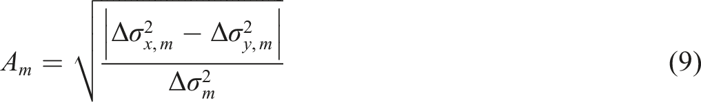$J_{m}$ at various scales by introducing an anisotropy indicator as

A_{m} = \sqrt{\frac{| Δ σ_{x, m}^{2} - Δ σ_{y, m}^{2} |}{Δ σ_{m}^{2}}}

(9)

where

Δ σ_{x, m}^{2}

represents the mean variance in the

x

-direction of

J_{m}

and

Δ σ_{y, m}^{2}

represents the mean variance in the

y

-direction. The indicator

A_{m}

ranges from 0 to 1, with 0 being isotropic and 1 being anisotropic (variation in

x

y

only). The anisotropy indicator is calculated for each tile for the four plan area indices

λ_{b}, λ_{i}, λ_{v}

and

λ_{w}

and averaged over all tiles belonging to the same neighbourhood type (Figure 10(e)-(h)). The anisotropy indicator is nearly identical for all neighbourhood types and land-cover types. The anisotropy is low at high resolutions and starts to increase significantly from a measurement scale of 62.5 m, with most anisotropy at the largest scale of 500 m (although note that at this scale there are only four cells in total and care must be taken in the interpretation of this value). As

{∆ σ}_{m}^{2} (λ_{w})

equals zero for tiles that contain no water, Figure 10(h) only shows anisotropy in the water neighbourhood type. The anisotropy of the water neighbourhood type is generally slightly larger than the anisotropy of the other neighbourhood types at the same scale, indicating that the different types of land-cover within the water neighbourhood type are more strongly anisotropic, as the land-cover types tend to be more aggregated in a single area (e.g., rivers, lakes, surrounded by green space, etc.) rather than distributed.

Conclusion

The heterogeneity of Greater London was investigated by calculating several morphometric indicators on neighbourhood-tiles of 1 km². The clear-cut positive correlation between the plan area index and fractal dimension of land-cover types (e.g., buildings) showed that fractal properties can be inferred from the plan area index without having to explicitly calculate the fractal dimension. The data suggests that when there is little area of a specific land-cover type, it is not distributed uniformly in space. For example, buildings are more likely arranged along a twisted road in sparse sub-urban areas, which corresponds to a fractal dimension above 1 but well below 2, filling the space more than a line but much less than a surface. It is not evident a priori that this should be the case and it is likely to be a consequence of urban design decisions rather than a natural process. With larger coverage, the land-cover type tends to be more homogeneously distributed, with a fractal dimension closer to 2. Moreover, evenness is negatively correlated to contagion, which suggests that areas with uniform proportions of different land-cover types also tend to be highly fragmented into many small patches rather than having each type clumped together individually. This is an important observation for the modelling of urban surfaces within weather and climate models, as it contradicts common practise to represent different land-cover types within a grid cell by separate fractions (called “tiles”) of uniform land-cover to model their effects on the atmosphere individually.

A clustering analysis with a subset of the morphometric indicators was used to describe city-scale heterogeneity. Whilst the analysis was purely based on the morphometric indicators, the resulting neighbourhood types also distinguished the functionality of the urban ecosystems (greenspace, residential, business districts, etc.). The clustering used the contagion index because of its weaker correlation to the other indicators. However, if this index is not available, the evenness would be a good substitute which can be directly calculated from the plan area indices of the surface cover, thus enabling a clustering analysis using only the most common indicators (plan area indices of buildings, impervious ground, vegetation, water, frontal area index of buildings). The frontal-area index is required to distinguish the dense and high-rise city centres (i.e., central business districts) from other parts of the core city. This distinction is important, as high-rise buildings significantly alter air flow at the ground level, can trap short- and long-wave radiation when forming narrow and deep street canyons, and affect the mixing properties with the atmosphere. In other parts of the city, the buildings’ frontal area index is similar to the plan-area index.

The neighbourhood types identified by the clustering algorithm have only weak associations with Local Climate Zones (LCZs), as the correspondence between them is not one-to-one and varies with resolution and grid boundaries. This may partially be due to a different set of parameters used in this study and the LCZs. The clustering approach is readily usable for other city contexts. It would be interesting to explore what the clustering algorithm would define and how these would link to LCZs. The approach towards classification of urban surfaces is also complimentary: LCZs are defined by a range of urban morphometric parameter values, as a result, a region at a certain scale usually falls into one specific LCZ type. In contrast, the clustering classification is based on the relative morphological similarity/dissimilarity, consequently, the results are purely data-driven (e.g., study domain, city context). Our analysis first classified the data, and the resulting clusters were then analysed according to their parameter values. This means that the clustering analysis may not always produce the same neighbourhood types or LCZ correspondence, but identifies for each city individually which categories are relevant. This can be an advantage in several cases: for example, for cities that do not correspond well the LCZs, or for research questions where the LCZ classes are too broad, but the clustering could further distinguish the landscape within one LCZ. We also added the contagion index to represent heterogeneity, and the clustering approach is more flexible towards including further parameters should they be relevant.

Multi-scale analysis and hierarchical decomposition of land-cover maps revealed the characteristic scales of land-cover types within the neighbourhood scale. The scale variance, which is the variance from the decomposed resolutions, indicates the most energetic scales and therefore where the most information gains lie. In this study, this is between 7.8 m (for vegetation, buildings) and 15.6 m (for buildings, roads), but at 250 m for water. It was shown that below measurement scales of 62.5 m, the neighbourhood types are homogeneous. Above this scale, neighbourhoods are anisotropic. One interesting finding is that all neighbourhood types and land-cover types reach similar levels of anisotropy, indicating that anisotropy of land cover is independent of land-cover type and land-cover fraction.

While any measure of heterogeneity generally depends on measurement scale, meaning that urban surface properties which appear heterogeneous at small scales will become homogeneous as the measurement scale increases, the hierarchical decomposition introduced in this paper conserves the total variance (i.e., the sum of the between-cell resolved variance and the averaged within-cell sub-grid variance) of the land-cover map. For numerical weather modelling, this gives important insight on the representation of urban environments at different scales. For example, if the resolved variance changes little by increasing the resolution, this implies that also the sub-grid variance remains similar, which in turn implies that the urban surface properties of a grid cell at that scale can be assumed to be statistically representative (i.e., the values do not significantly change upon small increases or decreases of the considered area).

There are several opportunities for future work. First, this study was limited to Greater London and it would be interesting to study other urban areas, especially developing cities. Second, due to the large number of potential input parameters for the clustering and the option of many different clustering algorithms, the results of the clustering will therefore depend to a certain extent on these choices. Third, environmental factors such as orography, temperature, wind velocity and air pollution are not considered at this stage to link the urban spatial heterogeneity with atmospheric modelling. Fourth, it may be possible to develop new heterogeneity indicators that provide different information and identify heterogeneity indicators that are independent of plan-area indices and each other as most heterogeneity indicators are related to the proportion or arrangement of urban constituents. In our analysis, the only direct heterogeneity indicator we used was contagion which measures the arrangement of one land-cover type. Last but not least, it would be valuable to study how multi-scale heterogeneous surfaces influence urban microclimate, the atmospheric boundary and regional weather.

Supplemental Material

Supplemental Material - Urban neighbourhood classification and multi-scale heterogeneity analysis of Greater London

Supplemental Material for Urban neighbourhood classification and multi-scale heterogeneity analysis of Greater London by Tengfei Yu, Birgit S. Sützl, Maarten van Reeuwijk in Environment and Planning B: Urban Analytics and City Science

Footnotes

Declaration of conflicting interests

The author(s) declared no potential conflicts of interest with respect to the research, authorship, and/or publication of this article.

Funding

The authors disclosed receipt of the following financial support for the research, authorship, and/or publication of this article: MvR is supported by the NERC highlight grant ASSURE: Across-Scale processeS in URban Environments (NE/W002868/1).

ORCID iDs

Birgit S Sützl

Maarten van Reeuwijk

Supplemental Material

Supplemental material for this article is available online.

Tengfei Yu has recently obtained his Master’s degree from the Department of Civil and Environmental Engineering at Imperial College London and his research project focuses on quantitative analysis of urban heterogeneity using GIS data and neighbourhood landscape classification. He obtained his Bachelor’s degree from Beijing Institute of Technology.

Birgit S. Sützl is a postdoctoral researcher at the Chair of Building Physics at ETH Zürich. Her research focuses on numerical modelling of urban climate, where she works on topics including: urban heat island mitigation measures, the influence of urban morphology on heat stress, urban heterogeneity, the representation of buildings in climate models, transport processes in the urban boundary layer, micro- and mesoscale models for urban environments. She obtained her PhD from Imperial College London working on modelling urban areas in Numerical Weather Prediction.

Maarten van Reeuwijk is a Professor of Urban Fluid Mechanics in the Department of Civil and Environmental Engineering at Imperial College London. He works on transport processes in urban areas (urban heat island, dispersion, microclimate), atmospheric convection, urban air quality and problems involving turbulent entrainment (volcanic releases, plumes/jets, clouds, ocean overflows, building ventilation). Much of his work focuses on multi-scale processes such as turbulence and how flow and turbulence interact with surfaces that have multi-scale features.

References

Allen

Lindberg

Grimmond

CSB

(2010) Global to city scale urban anthropogenic heat flux: model and variability. International Journal of Climatology 31: 1990–2005.

Barlow

(2014) Progress in observing and modelling the urban boundary layer. Urban Climate 10: 216–240.

Bartesaghi-Koc

Osmond

Peters

(2020) Quantifying the seasonal cooling capacity of 'green infrastructure types' (GITs): An approach to assess and mitigate surface urban heat island in Sydney, Australia. Landscape and Urban Planning 203: 103893.

Batty

Longley

(1994) Fractal Cities: A Geometry of Form and Function. London: Academic Press.

Berghauser Pont

Stavroulaki

Marcus

(2019) Development of urban types based on network centrality, built density and their impact on pedestrian movement. EPB: Urban Analytics and City Science 46: 1549–1564.

Best

Pryor

Clark

, et al. (2011) The Joint UK Land Environment Simulator (JULES), model description – Part 1: Energy and water fluxes. Geoscientific Model Development 4: 677–699.

Bohnenstengel

Evans

Clark

, et al. (2011) Simulations of the London urban heat island. Quarterly Journal of the Royal Meteorological Society 137: 1625–1640.

Boutle

Finnenkoetter

Lock

, et al. (2016) The London model: forecasting fog at 333 m resolution. Quarterly Journal of the Royal Meteorological Society 142: 360–371.

Buyantuyev

(2010) Urban heat islands and landscape heterogeneity: linking spatiotemporal variations in surface temperatures to land-cover and socioeconomic patterns. Landscape Ecology 25: 17–33.

10.

Cadenasso

Pickett

STA

McGrath

, et al. (2013) Ecological heterogeneity in urban ecosystems: reconceptualized land cover models as a bridge to urban design. In: Pickett

STA

Cadenasso

McGrath

(eds), Resilience in Ecology and Urban Design: Linking Theory and Practice for Sustainable Cities. Dordrecht: Springer, pp. 107–129.

11.

Cadenasso

Pickett

STA

Schwarz

(2007) Spatial heterogeneity in urban ecosystems: reconceptualizing land cover and a framework for classification. Frontiers in Ecology and the Environment 5: 80–88.

12.

Chen

Huang

(2018) Spatial measures of urban systems: from entropy to fractal dimension. Entropy 20: 991.

13.

Chen

Wang

Feng

(2017) Understanding the fractal dimensions of urban forms through spatial entropy. Entropy 19: 600.

14.

Clark

Mercado

Sitch

, et al. (2011) The Joint UK Land Environment Simulator (JULES), model description – Part 2: Carbon fluxes and vegetation dynamics. Geoscientific Model Development 4: 701–722.

15.

Crippa

Guizzardi

Pisoni

, et al. (2021) Global anthropogenic emissions in urban areas: patterns, trends, and challenges. Environmental Research Letters 16: 074033.

16.

Cullinan

Thomas

(1992) A comparison of quantitative methods for examining landscape pattern and scale. Landscape Ecology 7: 211–227.

17.

Dibble

Prelorendjos

Romice

, et al. (2019) On the origin of spaces: Morphometric foundations of urban form evolution. EPB: Urban Analytics and City Science 46: 707–730.

18.

Fernandez

Jelinek

(2001) Use of fractal theory in neuroscience: methods, advantages, and potential problems. Methods 24: 309–321.

19.

Fitch

PJR

Lovell

Davies

, et al. (2015) An integrated and quantitative approach to petrophysical heterogeneity. Marine and Petroleum Geology 63: 82–96.

20.

Fleischmann

Feliciotti

Romice

, et al. (2021) Methodological foundation of a numerical taxonomy of urban form. EPB: Urban Analytics and City Science 0: 1–17.

21.

Jochem

Leasure

Pannell

, et al. (2021) Classifying settlement types from multi-scale spatial patterns of building footprints. EPB: Urban Analytics and City Science 48: 1161–1179.

22.

Jochem

Tatem

(2021) Tools for mapping multi-scale settlement patterns of building footprints: An introduction to the R package foot. PLoS ONE 16: e0247535.

23.

Kent

Grimmond

Barlow

, et al. (2017) Evaluation of urban local-scale aerodynamic parameters: implications for the vertical profile of wind speed and for source areas. Boundary-Layer Meteorology 164: 183–213.

24.

Kodinariya

Makwana

(2013) Review on determining number of cluster in K-Means clustering. International Journal of Advance Research in Computer Science and Management Studies 1: 90–95.

25.

Lean

Barlow

Halios

(2019) The impact of spin-up and resolution on the representation of a clear convective boundary layer over London in order 100 m grid-length versions of the Met Office Unified Model. Quarterly Journal of the Royal Meteorological Society 145: 1674–1689.

26.

Reynolds

(1993) A new contagion index to quantify spatial patterns of landscapes. Landscape Ecology 8: 155–162.

27.

Reynolds

(1994) A simulation experiment to quantify spatial heterogeneity in categorical maps. Ecological Society of America 75: 2446–2455.

28.

Reynolds

(1995) On definition and quantification of heterogeneity. Oikos 73: 280–284.

29.

MacQueen

(1967) Some Methods for Classification and Analysis of Multivariate Observations. Euclid. Proc of Berkeley Symposium on Mathematical Statistics & Probability.

30.

Margairaz

Pardyjak

Calaf

(2020) Surface thermal heterogeneities and the atmospheric boundary layer: the thermal heterogeneity parameter. Boundary-Layer Meteorology 177: 49–68.

31.

Masson

(2000) A physically-based scheme for the urban energy budget in atmospheric models. Boundary-Layer Meteorology 94: 357–397.

32.

Mouzourides

Eleftheriou

Kyprianou

, et al. (2019) Linking local-climate-zones mapping to multi-resolution-analysis to deduce associative relations at intra-urban scales through an example of Metropolitan London. Urban Climate 30: 100505.

33.

Mouzourides

Kyprianou

Brown

, et al. (2014) Searching for the distinctive signature of a city in atmospheric modelling: Could the Multi-Resolution Analysis (MRA) provide the DNA of a city? Urban Climate 10: 447–475.

34.

Mouzourides

Kyprianou

Neophytou

MKA

(2013) A Scale-Adaptive Approach for Spatially-Varying Urban Morphology Characterization in Boundary Layer Parametrization Using Multi-Resolution Analysis. Boundary-Layer Meteorology 149: 455–481.

35.

Murwira

(2003) Scale matters!: a new approach to quantify spatial heterogeneity for predicting the distribution of wildlife. PhD Thesis. Wageningen: Wageningen University.

36.

Oke

Mills

Christen

, et al. (2017) Urban Climates. UK: Cambridge University Press.

37.

Ordnance Survey (GB) (2017) OS Master Map Topography Layer. UK. Scale 1:1000, Updated: May 2017, Using: EDINA Digimap Ordnance Survey Service https://digimap.edina.ac

38.

Ordnance Survey (GB) (2020a) OS MasterMap Topography Layer. Scale, 1: 1250. Updated: August 2020, Using: EDINA Digimap Ordnance Survey Service https://digimap.edina.ac

39.

Ordnance Survey (GB) (2020b) OS MasterMap Building Height Attribute. Scale 1: 2500. Updated: March 2020, Using: EDINA Digimap Ordnance Survey Service https://digimap.edina.ac.uk

40.

Ordnance Survey (GB) (2021) Boundary-Line. Scale 1:10000, Updated: April 2021, Using: EDINA Digimap Ordnance Survey Service https://digimap.edina.ac

41.

Pastor

(2005) Thoughts on the generation and importance of spatial heterogeneity in ecosystems and landscapes. In: Lovett

Turner

Jones

, et al (eds), Ecosystem Function in Heterogeneous Landscapes. New York, NY: Springer, pp. 49–66.

42.

Pickett

STA

Cadenasso

Jones

(2000) Generation of heterogeneity by organisms: creation, maintenance, and transformation. In: Hutchings

John

Stewart

AJA

(eds), The ecological consequences of environmental heterogeneity. London: Blackwell Science Ltd.

43.

Pickett

STA

Cadenasso

(2009) Altered resources, disturbance, and heterogeneity: A framework for comparing urban and non-urban soils. Urban Ecosystems 12: 23–44.

44.

Pickett

STA

Cadenasso

Rosi-Marshall

, et al. (2017) Dynamic heterogeneity: a framework to promote ecological integration and hypothesis generation in urban systems. Urban Ecosystems 20: 1–14.

45.

Pishro-Nik

(2014) Introduction to Probability, Statistics, and Random Processes. Kappa Research LLC. https://www.probabilitycourse.com.

46.

Pope

(2000) Turbulent Flows. Cambridge: Cambridge University Press.

47.

Qian

Zhou

Pickett

STA

, et al. (2020) Integrating structure and function: mapping the hierarchical spatial heterogeneity of urban landscapes. Ecological Processes 9: 59–69.

48.

Riitters

O'Neill

Wickham

(1996) A note on contagion indices for landscape analysis. Landscape Ecology 11: 197–202.

49.

Romme

(1982) Fire and landscape diversity in subalpine forests of Yellowstone National Park. Ecological Monographs 52: 199–221.

50.

Santos

Dodonov

Oshima

, et al. (2021) Landscape ecology in the Anthropocene: an overview for integrating agroecosystems and biodiversity conservation. Perspectives in Ecology and Conservation 19: 21–32.

51.

Stewart

Oke

(2012) Local climate zones for urban temperature studies. American Meteorological Society 93: 1879–1900.

52.

Strogatz

(2018) Nonlinear Dynamics and Chaos. Boca Raton, FL: CRC Press.

53.

Sun

Southworth

(2013) Remote sensing-based fractal analysis and scale dependence associated with forest fragmentation in an Amazon Tri-National Frontier. Remote Sensing 5: 454–472.

54.

Sützl

Rooney

van Reeuwijk

(2021a) Drag distribution in idealized heterogeneous urban environments. Boundary-Layer Meteorology 178: 225–248.

55.

Sützl

Rooney

Finnenkoetter

, et al. (2021b) Distributed urban drag parameterization for sub-kilometre scale numerical weather prediction. Quarterly Journal of the Royal Meteorological Society 147: 3940–3956.

56.

Tang

Lean

Bornemann

(2013) The benefits of the Met Office variable resolution NWP model for forecasting convection. Meteorological Applications 20: 417–426.

57.

Tannier

Pumain

(2005) Fractals in urban geography: a theoretical outline and an empirical example. Cybergeo: European Journal of Geography 307.

58.

Wiese

Stroup

Maiti

, et al. (2021) Measuring neighborhood landscapes: associations between a neighborhood's landscape characteristics and colon cancer survival. International Journal of Environmental Research and Public Health 18: 4728.

59.

Zhou

Pickett

STA

Cadenasso

(2017) Shifting concepts of urban spatial heterogeneity and their implications for sustainability. Landscape Ecology 32: 15–30.

60.

Zipper

Schatz

Kucharik

, et al. (2017) Urban heat island-induced increases in evapotranspirative demand. Geophysical Research Letters 44: 873–881.

Supplementary Material

Please find the following supplemental material available below.

For Open Access articles published under a Creative Commons License, all supplemental material carries the same license as the article it is associated with.

For non-Open Access articles published, all supplemental material carries a non-exclusive license, and permission requests for re-use of supplemental material or any part of supplemental material shall be sent directly to the copyright owner as specified in the copyright notice associated with the article.

0.00 MB

0.80 MB