Sage Journals: Discover world-class research

Abstract

Empirical study of road traffic collision (RTCs) rates is challenging at small geographies due to the relative rarity of collisions and the need to account for secular and seasonal trends. In this paper, we demonstrate the successful application of Hidden Markov Models (HMMs) and Generalised Additive Models (GAMs) to describe RTCs time series using monthly data from the city of Edinburgh (STATS19) as a case study. While both models have comparable level of complexity, they bring different advantages. HMMs provide a better interpretation of the data-generating process, whereas GAMs can be superior in terms of forecasting. In our study, both models successfully capture the declining trend and the seasonal pattern with a peak in the autumn and a dip in the spring months. Our best fitting HMM indicates a change in a fast-declining-trend state after the introduction of the 20 mph speed limit in July 2016. Our preferred GAM explicitly models this intervention and provides evidence for a significant further decline in the RTCs. In a comparison between the two modelling approaches, the GAM outperforms the HMM in out-of-sample forecasting of the RTCs for 2018. The application of HMMs and GAMs to routinely collected data such as the road traffic data may be beneficial to evaluations of interventions and policies, especially natural experiments, that seek to impact traffic collision rates.

Keywords

Road traffic collisions speed limits time series state-space models trend shifts

Introduction

The United Kingdom’s Department for Transport (DfT) reported that in the 12 months up to September 2018, 27,295 people were killed or seriously injured on British roads. Although deaths and injuries on the road have been declining locally and nationally (170,993 casualties in 2017 compared to 160,597 in 2018), as a preventable cause of death and disability, road traffic collisions (RTCs) remain an important policy priority.

A key in reducing the number of RTCs is a good understanding of their trend and seasonality. In particular, it is important for policy makers to be able to identify shifts in trend and associate them with possible causes. Accidents are the result of complex human behaviour influenced by multiple factors across micro–macro geographic and temporal scales. To model all of these would be impossible. In this paper, we present two different modelling approaches that provide valuable insights into the data generating process of RTCs using a minimal number of explanatory variables.

We take RTCs in Edinburgh as a case study. Our choice was motivated by the fact that in 2016 a 20 mph speed limit was introduced city-wide across Edinburgh by the City of Edinburgh council (Turley, 2014). It is a sign-only scheme and does not include physical traffic calming measures (Scotland, 2016). We investigate the effect of this policy on a city-wide scale, implicitly including spill-over effects on Edinburgh streets with no additional restrictions.

The 20 mph speed limit, which from now on we will refer to as the intervention, is a suitable example of an event that can potentially be associated with a structural change in the trend of RTCs and thus is of particular interest for the policy makers. A systematic review of the effectiveness of 20 mph speed limits is provided in Cairns et al. (2014) and Cleland et al. (2020).

The Hidden Markov Models (HMMs) discussed in this paper treat the time points of trend shifts as unknown. If, however, a shift in trend can be associated with one particular factor such as the speed limit intervention, the effect of this factor could be explicitly modelled using a different modelling approach – the Generalised Additive Model (GAM). GAMs allow for non-linear dependence in the covariates and thus provide more flexibility than standard modelling approaches such as Generalised Linear Models (GLMs).

The aim of this methodological paper is to provide additional valuable tools to the methods commonly used to aid decision-makers in the evaluation of natural experiments. In particular, we introduce methods to detect shifts in the trend of a time series and to assess the influence of potential contributing factors. Our methodology enables a wider range of research questions to be asked when faced with small samples of longitudinal outcome measurements, adopting extensive model discrimination procedures which include forecast-ability of the models considered. In addressing the challenges of modelling outcomes such as RTCs at smaller scales like individual cities, we gain an understanding of the trends and seasonality of the RTCs in Edinburgh as well as the effects of the 20 mph speed limit policy that was introduced in 2016.

The sparse presentation of the modelling approach common in the planning literature related to 20 mph speed limits in the UK (for example Grundy et al., 2009) is of limited help to the practitioners. This is why we have taken the effort to make our methods transparent and reproducible by providing sufficient detail.

Approaches commonly used for modelling RTCs and related phenomena

Key approaches to modelling RTCs and related phenomena include Autoregressive Integrated Moving Average (ARIMA) models, Poisson count models, Negative Binomial models, Multivariate/Binomial logistic models, HMMs and GAMs.

ARIMA models are important for quantifying the trend in collisions (by week/month/year), facilitating forecasting of collisions and assessing for seasonality. This type of model has been implemented for modelling data on accidents from various countries (Mehmandar et al., 2016; Yousefzadeh-Chabok et al., 2016), for forecasting the trend in road collision mortality and assessing road traffic injury trends (Friedman et al., 2007), for assessing the impact of raised speed limits on road traffic fatalities (Rodríguez et al., 2015), and assessing road traffic injury trends, and assessing and predicting road accident injury (Parvareh et al., 2018).

Poisson models are commonly used for modelling road collision data since the data are counts (Akin, 2001; Roshandeh et al., 2016). However, in many cases the data are overdispersed, and Poisson models are not ideal. In contrast, Negative Binomial models facilitate the modelling of count data when that data are overdispersed. In a recent study on the effects of 20 mph speed limits in Bristol Bornioli et al. (2020), Negative Binomial regression was applied to demonstrate the significant effect of the intervention on the reduction of fatal injuries. Both Poisson and Negative Binomial models are applied in Akin (2001).

HMMs are important for assessing underlying mechanisms for generating the observed data and are suitable for overdispersed, and autocorrelated data (Zucchini et al., 2016). These models, also known as Hidden Markov Processes or Markov Switching models, are another option for modelling count data such as the number of RTCs per month. Through the introduction of a latent layer, these regime-switching models naturally accommodate long-term structural changes. HMMs have been adopted by researchers for assessing vehicle trajectories (Saunier and Sayed, 2006), for modelling traffic incidents at intersections (Jun et al., 2013), for modelling Vehicular Crash Detection (Singh and Song, 2009) and for vehicle collision prediction (Xiong et al., 2018).

GAMs facilitate modelling count data such that the explanatory variables are incorporated into the model in the form of smooth functions, allowing for non-linear relationships to be considered in the modelling process. A GAM can be considered as an extension of a GLM. GAMs have been used for estimating motorcycle collisions (Machsus et al., 2015) and for accident frequency analysis (Xie and Zhang, 2008).

Other approaches in RTCs research include those which focus on assessing the impact of key factors on the frequency of RTCs such as Lord and Mannering (2010), assessing the probability of injury severity of drivers with discrete choice models such as ordered Probit and mixed Logit models (Chen and Chen, 2011; Chen et al., 2019; Dong et al., 2018), assessing individual transport corridors (Kolody et al., 2014) and investigating the likelihood of RTCs by the hour (Chen et al., 2018).

To date, RTCs in the UK have not been modelled with either HMMs or GAMs; the focus has been on Poisson based models. Modelling approaches already used include Space–time multivariate Bayesian models (Boulieri et al., 2017), Zero Truncated Bivariate Poisson models (Chowdhury and Islam, 2016), Generalized linear models, Generalized estimating equations, Hierarchical generalized linear models (Memon, 2012) and interrupted time series models (Grundy et al., 2009).

Extending the focus to time series models such as HMMs and GAMs introduces a larger scope for enquiry into the RTC temporal trends. Our methods extend that done by Grundy et al. (2009) by facilitating the detection of structural changes in the temporal trend, and facilitating the detection of non-linear patterns in the temporal trend.

The detection of latent temporal shifts in RTCs has not been addressed in the modelling approaches in the literature so far; in addition, non-linear estimation of the temporal trend has not been addressed either. In this paper, we address both of the above-mentioned goals.

Data

The dataset used for the analyses in this paper is the road safety data compiled by the DfT from STATS19 accident report forms that are completed by the police for any collisions involving person injury in Great Britain (source: https://www.gov.uk/government/collections/road-accidents-and-safety-statistics). In particular, we investigate the monthly total count of RTCs, which happened in the City of Edinburgh (citywide) for the period for which we have available data: April 1996 until December 2018 (we subset the data for the UK by setting LAD # = 923). Edinburgh is the capital city of Scotland, with a central Old Town including buildings data back to the medieval period and an adjacent Georgian New Town, surrounded by suburbs. In 2017, the population of the city was estimated to be 513,210 (source: https://www.edinburgh.gov.uk/strategy-performance-research/edinburghs-population?documentId=12754&categoryId=20202), living across an area of around 264 km². The city is home to businesses and industry as well as a popular tourist destination, with major festivals in August and December/January.

We have 273 monthly observations in total, 30 of which are after the intervention. We divide this in two samples – a training and a validation. The training sample ends in December 2017 and has 261 observations, 18 of which are after the intervention. We use this sample for fitting models. The validation sample consists of the 12 monthly RTCs in 2018 and is used for evaluating out-of-sample forecasting performance of the chosen models. We note that from the viewpoint of the complexity of the models we use in our analyses, our (training) sample size, i.e. the number of time points, is small.

Figure 1 plots the total time series of RTCs in the City of Edinburgh for the study period. The solid bar indicates the time point of the intervention – July 2016, while the dashed bar indicates the start of the validation sample. Visual inspection suggests dependence in the data and a decreasing trend. There seems to be a further decrease in the trend after the intervention but a more formal approach is needed to strengthen this statement.

Figure 1.

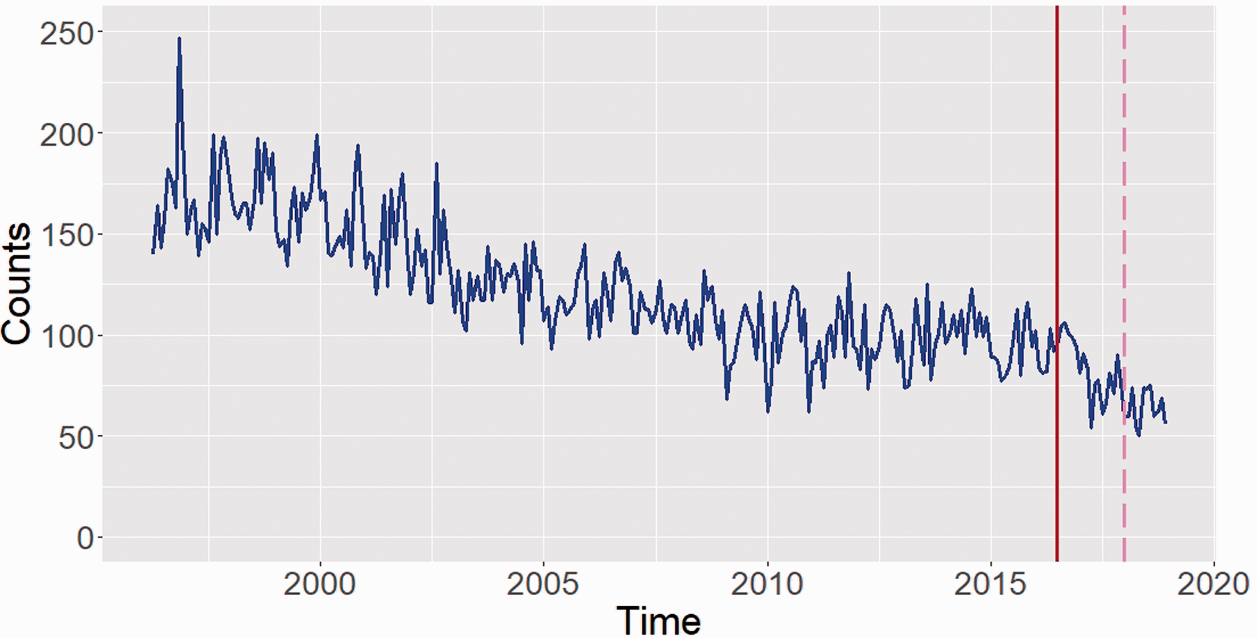
Time series of monthly counts of road collisions in Edinburgh. The solid bar indicates the time point of the intervention – July 2016. The dashed bar indicates the start of the validation sample – January 2018.

To gain further insights, we plot in Figure 2 the mean RTCs per month divided by the number of days for the respective month (leap years are ignored for this calculation), i.e. we plot the mean RTC rate per day for each month. The plot gives a crude idea of potential seasonality. There seems to be a peak in the autumn months, while the start of the year tends to be calmer. We also observed an isolated peak in August, which might be attributable to the increase in traffic during the Fringe festival in Edinburgh.

Figure 2.

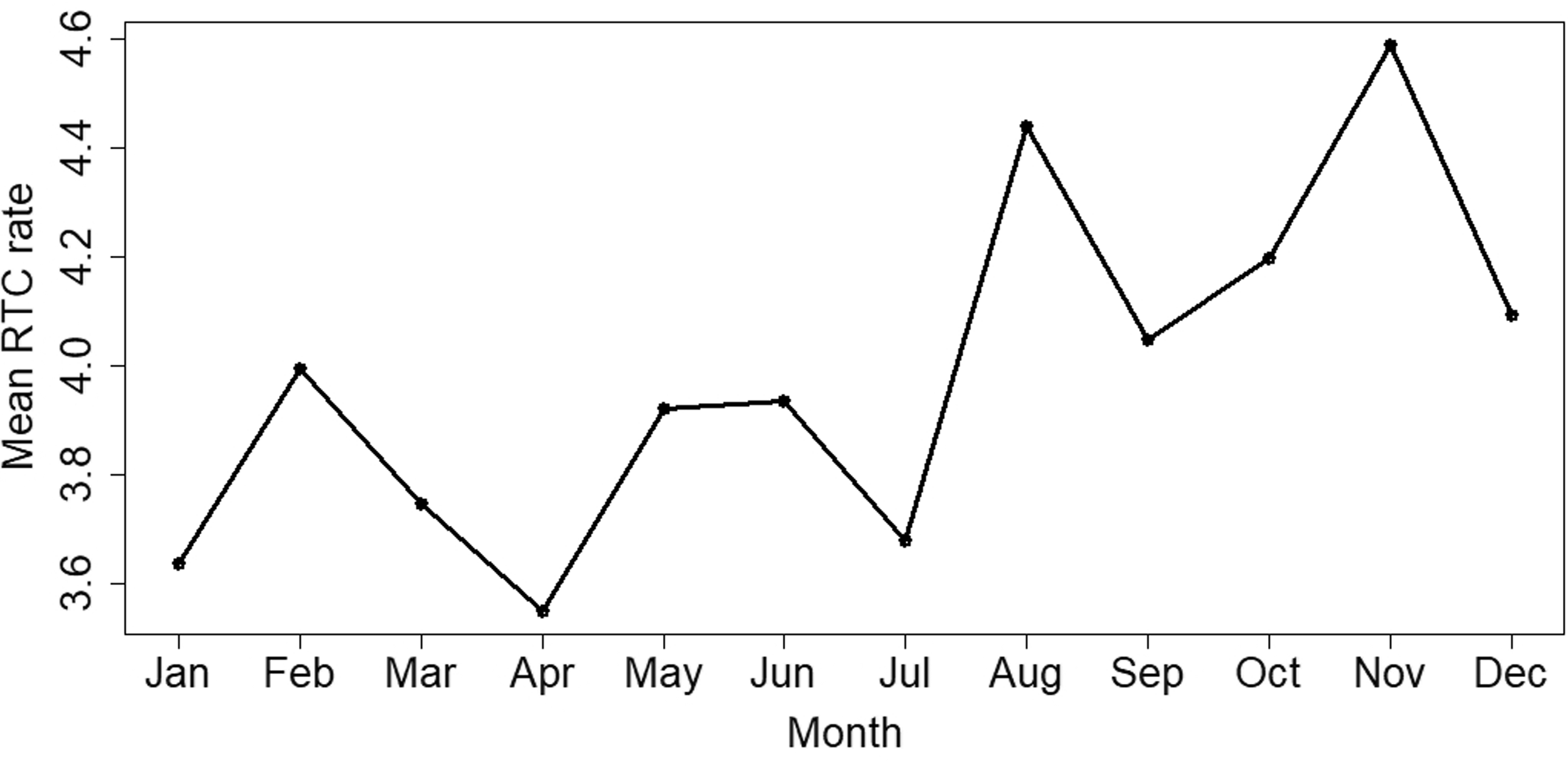
Mean RTCs for each month divided by the number of days for the respective month (mean rates).

This early exploratory analysis shows indications for serial dependence, trend and seasonality, which will be addressed in the methodology section.

Methodology

Hidden Markov Models

In their nature HMMs are time series models, which automatically make them a suitable candidate. They account for dependence in the data through the latent Markov Chain. They are flexible and could be tailored for many real-world applications. In particular, incorporating trend and seasonality is straight-forward (see equation (2)). Moreover, the distributions of forecasts could be easily obtained as discussed in the Section ‘Estimation, model selection, diagnostics, decoding and forecasting’. In addition, the latent states could be decoded, which in turn could provide useful insights into the data-generating process. Most importantly, through the latent layer of states one can detect shifts in the trend without explicitly accounting for potential explanatory variables, which may be difficult to obtain.

HMMs are stochastic processes containing two components – an observable time series influenced by an underlying latent state sequence. In our case the observable process produces realisations of the RTCs. It is assumed that at each time point the system could be in one of N possible states indicated by the hidden process. The latter follows a Markov Chain satisfying the memorylessness property that given the current state, future values are independent of the past. The random variables from the observable process are assumed to be drawn from N distributions, where the latent state process determines which of these distributions is ‘switched on’ at each time point. For this reason, the distributions are called ‘state-dependent distributions’ and are usually assumed to come from the same distributional family (see Langrock et al. (2015) for a non-parametric approach). Conditional on the current state, the respective observable random variable is independent of all past (and future) observations and states.

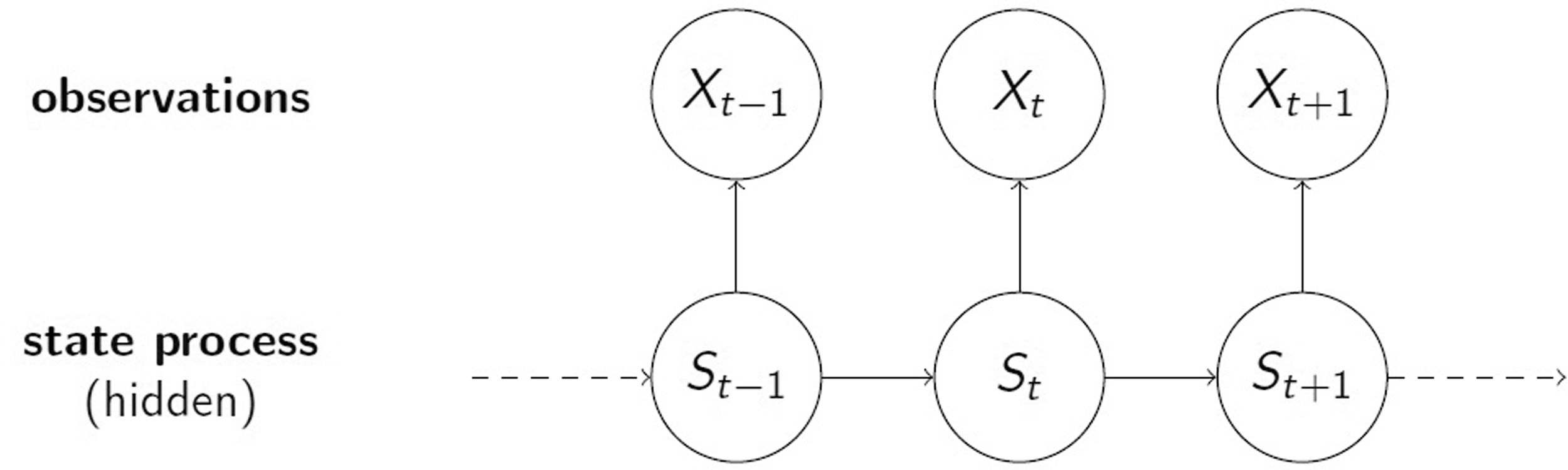
In the following we denote the observable state-dependent process by X_t, $t = 1, \dots, T$ with T being the sample size, and the underlying latent $N -$ state Markov Chain by S_t. The two components and their dependence structure are visualised in Figure 3. Given the limited data set, we consider HMMs with N = 2 states but also checked in the empirical study whether more than two states are required.

Figure 3.

Visualisation of an HMM. Arrows indicate dependence. S_t denotes the state process, while X_t denotes the observable one.

The specification of HMMs can be broken down into two parts – specification of the Markov Chain and specification of the state-dependent distributions. Here we provide a short summary of these specifications. Details can be found in the Supplementary material.

A Markov Chain is characterised by the initial distribution $δ$ , i.e. the probabilities of each state when we start observing the process, and by transition probabilities $γ_{i j}^{t} : = P (S_{t} = j | S_{t - 1} = i)$ summarised in the transition probability matrix (t.p.m.)

Γ = (\begin{matrix} γ_{11} & γ_{12} \\ γ_{21} & γ_{22} \end{matrix}) = (\begin{matrix} 1 - γ_{12} & γ_{12} \\ γ_{21} & 1 - γ_{21} \end{matrix})

(1)

γ₁₁ and γ₂₂ give the probabilities of staying in the same state – State 1 and State 2, respectively, while γ₁₂ and γ₂₁ provide the probabilities for a shift.

For the state-dependent distributions, we first specify the distributional family. Since we are modelling counts, a suitable candidate is the Negative Binomial (NB) distribution. It has the advantage of a size parameter controlling the variance and therefore allowing for overdispersion within the states. We consider two further distributional families – Poisson and Normal. The Poisson distribution is a popular choice when modelling counts. It offers less flexibility than the NB distribution as its variance strictly equals the mean. Noting that the counts are relatively large numbers taking a wide range of values, one could alternatively use the Normal distribution as an approximation.

Irrespective of the choice of distributional family for the counts of RTCs, we model the mean taking a GLM approach. In particular, we use a log link to express the mean as follows

log (μ_{t, i}) = log (day s_{t}) + a_{i} + b_{1, i} t + b_{2} \cos (2 π t / 12) + b_{3} \sin (2 π t / 12),

(2)

with

i = 1, \dots, N

and

t = 1, \dots, 261

log (day s_{t})

is the offset. a_i and

b_{1, i}

are the intercept and the slope of the trend lines associated with each state. A switch between the states would therefore lead to a switch in the trend. For completeness in our empirical study we consider a model with a constant slope across the states, i.e.

b_{1, 1} = b_{1, 2} = b_{1}

. We refer to this model as a ‘constant trend’ model. In simple words, such a model accommodates a step change in the expected number of RTCs without affecting the trend. Note that we implicitly assume that the seasonal pattern controlled by the parameters b₂ and b₃ is constant across the states. This is done out of necessity given the small sample size but we also find this assumption reasonable. Any changes are more likely to affect the trend rather than the seasonality. We also note that a constant seasonal pattern facilitates the interpretation of the states.

If the research interest lies in studying the influence on the trend of one particular factor such as the intervention, it can be added within the framework of HMMs as a further explanatory variable in the mean model for the state-dependent distribution (equation (2)). We explore this modelling approach in the Supplementary material. Here we note that we found no compelling evidence for the advantage of this alternative. This is not surprising. We would expect the intervention to have an effect either on the Markov Chain as a cause of a structural change, or on the state-dependent distribution but not necessarily on both.

Estimation, model selection, diagnostics, decoding and forecasting

We use a Maximum Likelihood approach for the estimation of the model parameters. A brute force approach to calculating the likelihood would require summation over all possible states at each time point, which becomes infeasible even for moderate sample sizes. Tractability of the likelihood is achieved using the so-called forward algorithm – see Zucchini et al. (2016) for details. The parameters in the likelihood are estimated using Newton–Raphson-type numerical optimisation of the log likelihood. This is implemented in the software R (R Core Team, 2018) using a bespoke code based on the routine nlm.

We use the Akaike Information Criterion (AIC) and Bayesian Information Criterion (BIC) to choose between the candidate models. One way of checking the adequacy of the model is using pseudo-residuals. For details about the calculation of these, see Zucchini et al. (2016).

The crucial part in our analysis is decoding the states to allow us to detect shifts in the trend. For this purpose, we use a procedure known as the Viterbi algorithm (see Zucchini et al., 2016) that allows us to obtain the sequence of states with the highest probability given the data.

Using the concept of forward probabilities which is in the core of the forward algorithm, one can obtain the distribution of the h-step-ahead forecasts of the observable variable X_t –see Zucchini et al. (2016). From this distribution point and interval forecasts can be easily produced.

Generalised Additive Models

The HMM from the previous section allows us to detect shifts in the trend, which can be associated with the intervention. However, when the primary interest of the policy makers lies in the explicit modelling of the intervention effect, GAMs (Wood, 2016) provide a suitable alternative.

A GAM for the RTC data could be specified as follows. Let X_t be a random variable for the RTCs such that $X_{t} \sim N B (μ_{t}, n)$ and

log (μ_{t}) = log (day s_{t}) + f_{t r} (t) + f_{seas} (s)

with

t = 1, \dots, 216

and

s = 1, \dots, 12

log (day s_{t})

is as before an offset term, f_tr and f_seas are smooth functions with cubic spline basis for the trend and for the seasonality features, respectively. Detail on constructing splines is provided in Wood (2016). We note that f_seas is cyclic cubic regression spline with k = 12 knots to ensure continuity at the end points of the spline. The basis dimension of f_tr is set to 10 – the default suggested in Wood (2016). In our empirical study, we checked whether this dimension is sufficiently high using a residual randomisation test.

Incorporating the effect of the intervention, the mean equation could be modified as follows

log (μ_{t}) = log (day s_{t}) + f_{t r, 1} (t) + f_{seas} (s) + d_{t} f_{t r, 2} (t),

where, as before

t = 1, \dots, 261

and

s = 1, \dots, 12

and d_t is a dummy variable taking the value zero for

t = 1, 2, \dots, 243

and 1 otherwise. This is in fact a smooth-factor interaction between the trend and the dummy-variable d_t.

f_{t r, 1}

gives effect of the trend without the intervention,

f_{t r, 2}

gives the additional effect of the intervention on the trend. If the term is significant and leads to a further decline of the trend, then this provides evidence that the policy of limiting the speed to 20 mph in the city of Edinburgh has been successful.

We fit the model using the gam function from the mgcv package (Wood, 2016). A restricted Maximum Likelihood estimation is applied.

For model selection (between GAM models), a corrected AIC is used as defined in Wood (2016: 304).

Diagnostics were performed using residual plots and tests on the deviance residuals. In particular, we look at quantile–quantile plots and residual versus fitted values plots to see if there are any patterns unexplained by the model. We also check the autocorrelation in the residuals.

Using the underlying parametric representation of a GAM model, one can obtain a ‘prediction matrix’ based on the covariates. Together with the estimated coefficients, the prediction matrix could be used for forecasting (Wood, 2016). In R we use the command predict with the argument type=“response” to produce forecasts on the response scale.

Empirical study

In an empirical study, we fit the HMMs and the GAMs to the RTC data and run model selection, model diagnostics and forecasting evaluation. We start with fitting HMMs to the data.

Hidden Markov Models

There is a wide variety of candidate models within the HMM framework. In particular, we have to make a decision regarding the distributional family of the state-dependent distributions, the number of states and whether we will allow the slope of the trend to vary across the different states.

For this purpose, we consider six models in total. First we fit two-state HMMs with NB, with Poisson and with Normal state-dependent distributions. For these models, we keep the effect of both the trend slope and seasonality constant across the states. Based on the best fit, we investigate whether increasing the number of states brings an improvement. Finally we consider models when the trend slope varies across the states (but the seasonality remains constant as discussed above). The likelihoods and the model selection criteria for the six models are given in Table 1.

Table 1.

Negative Log-likelihood (nllk), AIC and BIC for the seven HMMs.

Model	nllk	AIC	BIC
HMMs with constant T and S
Two-state NB	1070.26	2158.51	2190.59
Two-state Poisson	1086.49	2186.97	2211.92
Two-state Normal	1073.85	2165.69	2197.77
One-state NB	1086.56	2183.11	2200.93
Three-state NB	1067.28	2164.56	2218.03
Two-state NB HMM with varying T
Varying T	1067.33	2154.66	2190.31

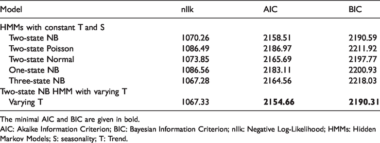
The minimal AIC and BIC are given in bold.

AIC: Akaike Information Criterion; BIC: Bayesian Information Criterion; nllk: Negative Log-Likelihood; HMMs: Hidden Markov Models; S: seasonality; T: Trend.

From the three candidate distributions, the NB is preferred. Note that the Normal distribution provides a reasonable approximation. One state is not enough to explain the data, which indicates that the trend is not constant. Note that the 1-state HMM is in fact a GLM, which indicates that a non-trivial HMM is preferred over simpler models. In addition, more than two states are not justified even for the simplest models. Based on both model selection criteria the best model is a 2-state NB with varying trend and constant seasonality.

Model fit and diagnostics for the best model

In this section, we investigate the model fit of our preferred HMM. First we check the adequacy of the fit with the pseudo-residual segments. A plot is provided in Supplementary material Figure 1. We do not spot any particular problems as most segments are within the 99% confidence boundaries. Therefore, there are no clear indications for inadequacy of the fit.

Summaries of the estimates of the intercept and the trend coefficients in equation (2) are provided in the Supplementary material. We note here that there is a significant negative trend. The estimates of the trend coefficients for each state do not lie in the confidence intervals for the trend parameter of the other state, which confirms that there is a significant difference in the effect of trend across the states.

To facilitate the interpretation of the estimated trend coefficients and to gain a better understanding of the states, we plot the fitted values for both states in Figure 4.

Figure 4.

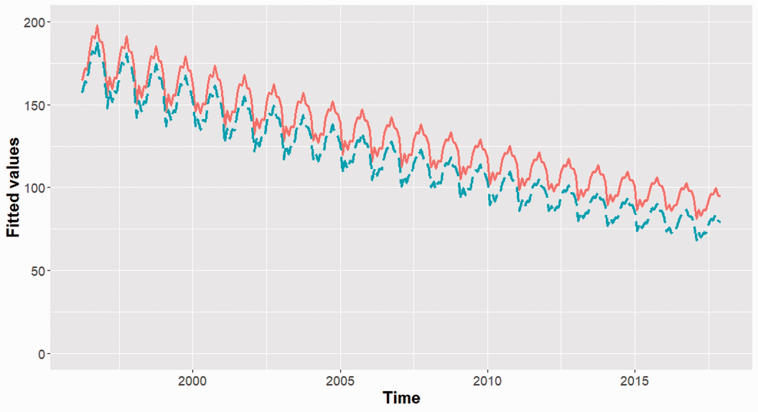
Two-state NB HMM with varying trend, constant seasonality and no intervention effect: fitted values for the two states. Solid line is for state 1 and dashed line is for state 2.

State 1 starts with a slightly higher expected number of RTCs and its decline over the years is slower. Based on the plot we cautiously label state 1 as a ‘slow-decreasing-trend’ and state 2 as a ‘fast-decreasing-trend’ state.

The contribution of each month to the log rate is plotted in Figure 5. Ceteris paribus, accident numbers seem to peak in early autumn and are lowest in early spring. This result confirms our findings in the exploratory analysis (Figure 2).

Figure 5.

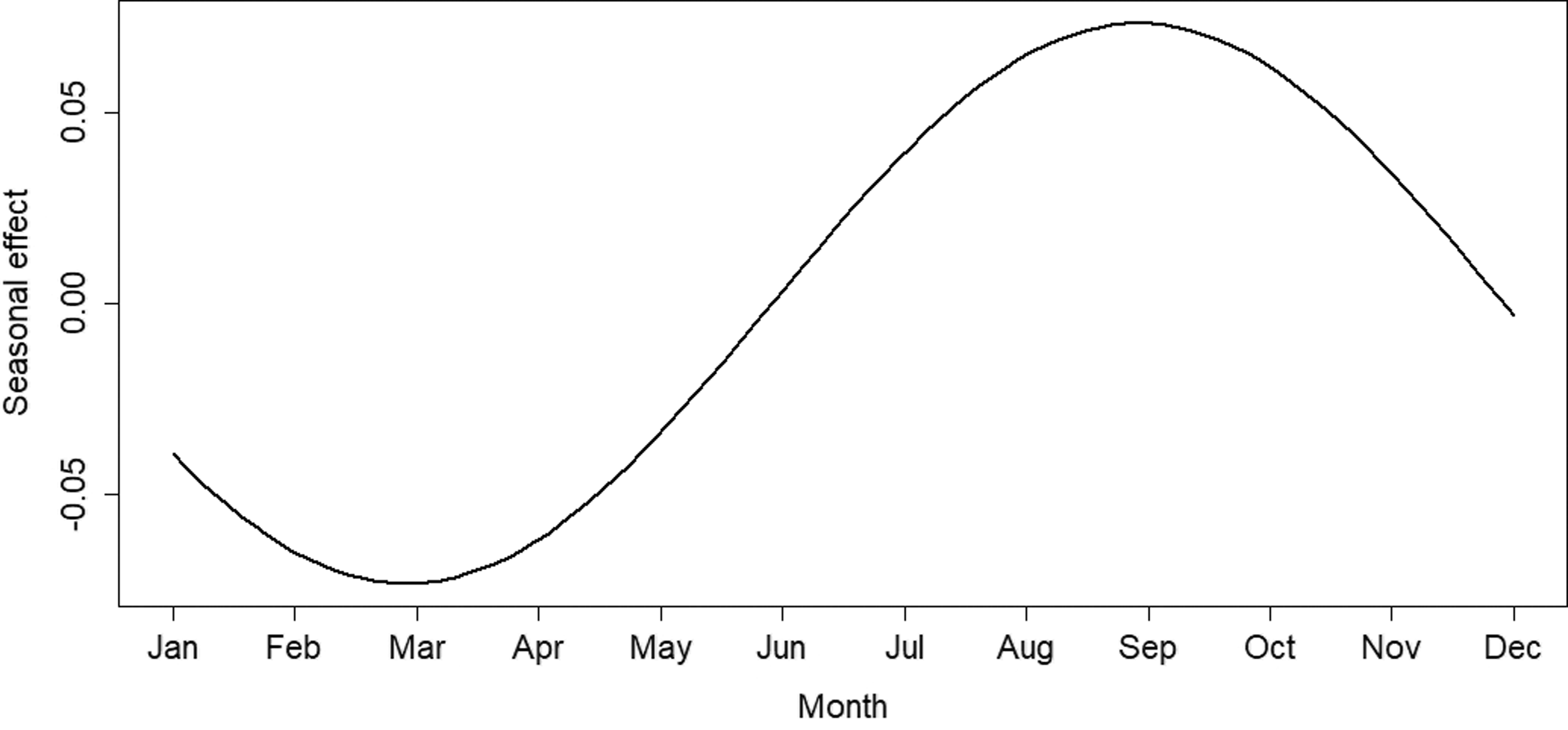
Two-state NB HMM with varying trend and constant seasonality: contribution of each month to the log mean.

The estimated t.p.m. is

\begin{matrix} \hat{Γ} = (\begin{array}{l} {\hat{γ}}_{11} {\hat{γ}}_{12} \\ {\hat{γ}}_{21} {\hat{γ}}_{22} \end{array}) = (\begin{array}{l} 0.9624 (0.9470, 0.9973) 0.0376 (0.0027, 0.0530) \\ 0.0123 (0.01, 0.1306) 0.9877 (0.8694, 0.99) \end{array}) \end{matrix}

The states are very persistent and switches occur rarely – between 1% and 3% of the time (depending on the state). Persistent states (high probability of staying in the same state) can be reasonably explained by a slow changing data-generating process with the rare switches between the states corresponding to non-observable structural changes. In our model, switches correspond to trend shifts. The indication that these occur rarely is in line with our expectations.

The key question is to find when the trend shifts took place. We address this using the global decoding procedure – the results are given in the upper plot in Figure 6.

Figure 6.

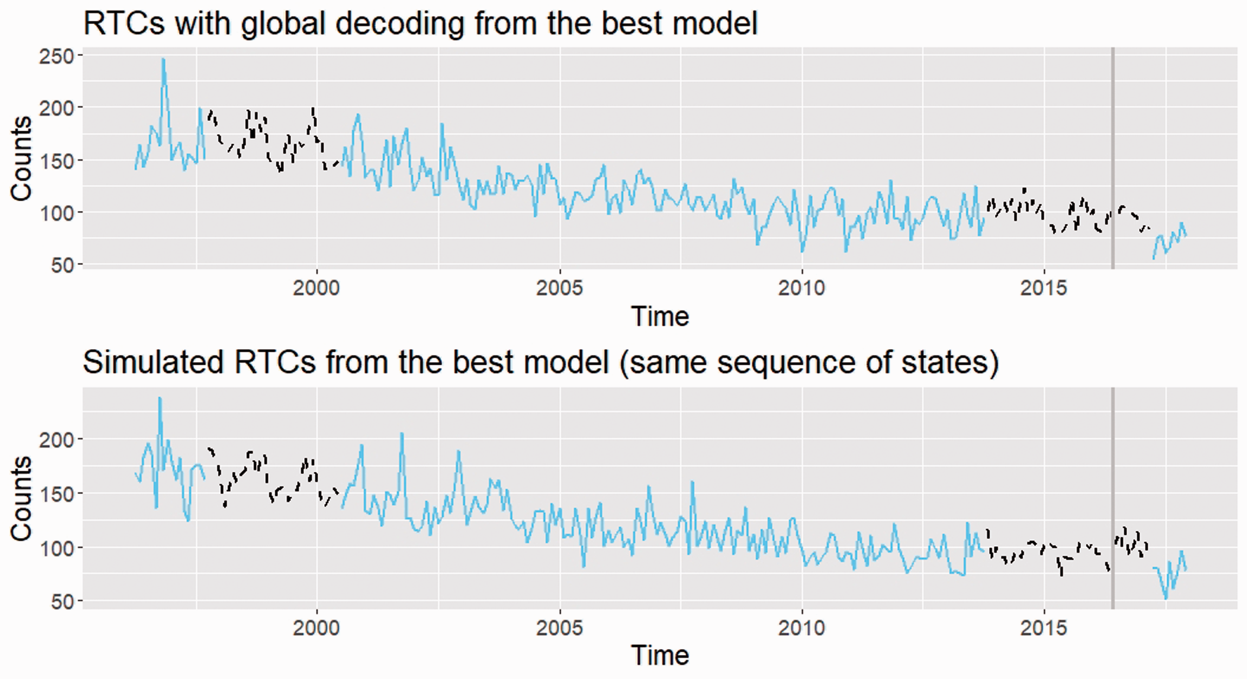
Decoding of the states and a simulated sample. State 1 (‘slow-decreasing state’) is in dashed line, while state 2 (‘fast-decreasing state’) is in solid line.

The states are indeed persistent with the system tending to stay slightly longer in the ‘fast-decreasing-trend’ state 2. For the 261 months we observe four transitions, which is in line with the estimates for γ₁₂ and γ₂₁. The four trend shifts occur in October 1997 (fast to slow), July 2000 (slow to fast), November 2013 (fast to slow) and April 2017 (slow to fast).

It is not always possible to associate a trend shift with a particular event. There are many factors working in the background and their interaction might have caused the slowing or the acceleration of the decreasing trend. At the moment we do not have an explanation for the first three shifts. However, the last trend shift – the one in April 2017 – occurred several months after the intervention. The result can be used as an indicator for the policy makers that the 20 mph limit was a success.

Note that using HMM to detect a trend shift could be a cue to explore potential explanations, especially if the shift indicated an increase in RTCs.

If the policy makers are interested in an explicit modelling of the effect of the intervention, GAMs provide a better alternative.

Before we investigate this in more detail, we run a further diagnostic check using simulations from the fitted model. For the purpose of comparison, we use the decoded state sequence for the simulation. The simulated time series of RTCs is given in the lower plot of Figure 6. The simulated data seem to reflect well the observed process. In particular, it captures the declining trend and the formation of a ‘trough’ in the later years of the observation period.

GAMs

Two GAMs – one with and one without intervention – are fitted to the data using the R package mgcv. The corrected AIC of the GAM with intervention (2115.456) is lower than the corrected AIC of the model without intervention (2116.385). This provides us with some confidence to work further with the former model.

We start with running some diagnostic checks on the fit. Detailed information is given in the Supplementary material. Here we note that the fit is reasonable.

The model fit reveals that the smooth terms for the trend, for the seasonality and for the additional effect on the trend are all highly significant (the three p-values are <0.001), which provides further evidence for the statistical significance of the effect of the intervention. We plot the three smooths in Figure 7. The GAM has correctly captured the declining trend including the ‘trough’ in later years. The seasonal pattern is very similar to the one in Figure 2 from the exploratory analysis. The key finding is that the effect of the intervention is to further decrease the number of RTCs. Thus the GAM also indicates that the introduction of the 20 mph limit policy in the City of Edinburgh was successful.

Figure 7.

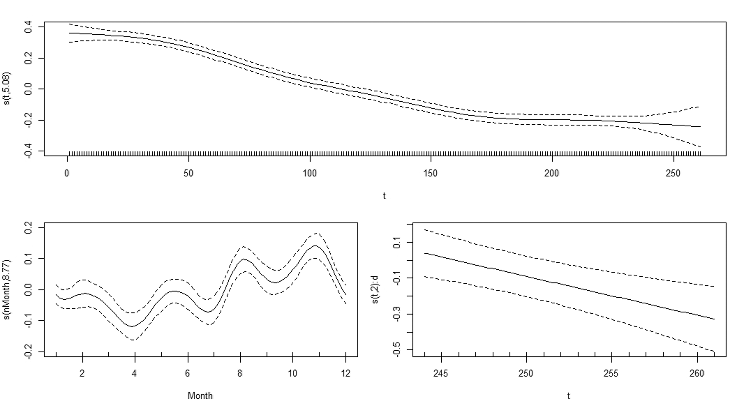
Fitted smooths. Upper plot gives the smooth for the trend, lower left plot gives the smooth for the seasonality, lower right plot gives the smooth for the additional effect of the intervention.

Forecasting

HMMs and GAMs helped us learn about the trend, seasonality and the impact of the intervention on the RTCs in Edinburgh. Both approaches serve different purposes in our study – detecting shifts in the trend for the HMMs and explicit modelling of the intervention for GAMs – but a natural question is how do the two models compare to each other. We address this question by using forecasts as a comparison measure for the performance of the best performing HMM and GAM from the model fits. In particular, we take advantage of the 12 observations for 2018 to make one-step-ahead out-of-sample forecasts and evaluate the performance of the two models using the Mean Squared Error (MSE) measure.

Table 2 gives the observed values and the two sets of forecasts for each month in 2018 as well as the MSE. The GAM has a much lower MSE than the HMM, which can be attributed to the fact that the HMM tends to overestimate the RTCs in the last few months of 2018. We conclude that the GAM proves more valuable in making out-of-sample forecasts.

Table 2.

A table with the observed RTCs and the forecasts from the selected HMM and GAM.

Month	RTCs	HMM	GAM
1	60	76	66
2	60	66	58
3	74	71	60
4	55	68	54
5	50	70	60
6	74	70	57
7	73	75	55
8	75	78	63
9	60	78	56
10	62	81	58
11	69	77	59
12	56	77	51
MSE	–	171.56	102.69

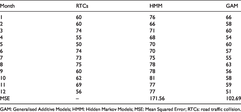
GAM: Generalised Additive Models; HMM: Hidden Markov Models; MSE: Mean Squared Error; RTCs: road traffic collision.

To consolidate our findings about the intervention effect, we calculate the MSE of the forecasts obtained from the GAM without intervention. This MSE was 126.11, which is higher than the MSE of the forecasts from the GAM with intervention. This provides further evidence for the intervention effect.

Discussion

In this paper we apply and critically appraise two modelling approaches – HMMs and GAMs – to develop our understanding of the systems that determine RTCs and to evaluate changes and interventions within those systems.

The reduction of RTCs is a ‘real-world’ problem for which the analytical tools for assessment deal with primarily, count data. Here, we demonstrate successfully, both the application and advantage of using HMMs and GAMs in evaluations conducted within a public health natural experiment framework. Moreover, we have suggested techniques that can be used in local government to learn about the shifts in RTC trends and to identify when an intervention may be required – for example when the HMM indicates a slowdown in the decreasing trend.

HMMs are gaining popularity in modelling time series in numerous areas of research, including ecology (Popov et al., 2017), finance (Rogers and Zhang, 2011) and medicine (Langrock et al., 2013) to name just a few. From modelling perspective, the advantages of HMMs lie in their intuitive appeal, the mathematical tractability of the likelihood function and the flexibility of extending the baseline model. From the perspective of the policy makers HMMs can be used as an exploratory tool to identify shifts in trend using the procedure of global decoding. In our case study, we focused on a well-known intervention and demonstrated that the trend moved from a slow-decreasing to a fast-decreasing state several months after its introduction. In other applications, the time points of switches between the latent state trends can potentially be linked to previously unidentified and modifiable determinants of collisions.

When the main interest lies in modelling the effect of the intervention, GAMs (Wood, 2016) provide an alternative modelling approach that captures non-linear patterns using splines. These models can be easily adapted for time series data.

We draw two major conclusions from our study. First, both HMMs and GAMs could reliably model time series of RTCs when the main goal is to reflect the trend and the seasonal patterns observed in the data. In terms of assessing the effect of intervention, the GAM was our preferred approach because of the better model fit and forecasting success. Second, there is compelling evidence that, following the 20 mph policy in Edinburgh a further reduction in collision rates in this city occurred. This is a significant result for overall public health in the City of Edinburgh and can spur on similar policies in other cities in the United Kingdom.

It is worth noting, however, that there are a number of covariates that can potentially influence the RTCs: other activities occurring in the City such as the cycling and walking initiatives in the City of Edinburgh, the fluctuating changes in fuel prices, general attitude towards alcohol consumption, etc. As with the intervention, we have only considered them implicitly within the HMM framework by allowing structural changes in the data-generating process. Future studies may focus on quantifying them and when a richer data set is available – implementing such covariates in the modelling approaches outlined in this paper.

Finally, there is no reason why HMMs and GAMs should only be viewed as competing models. Both approaches can be successfully combined in an HMM with smooth functions of the covariates in the state-dependent distributions (Langrock et al., 2017). Our sample size is too small for such a complex model but once more data are available this path could be explored in future research.

Supplemental Material

sj-pdf-1-epb-10.1177_2399808320985524 - Supplemental material for Trend shifts in road traffic collisions: An application of Hidden Markov Models and Generalised Additive Models to assess the impact of the 20 mph speed limit policy in Edinburgh

Supplemental material, sj-pdf-1-epb-10.1177_2399808320985524 for Trend shifts in road traffic collisions: An application of Hidden Markov Models and Generalised Additive Models to assess the impact of the 20 mph speed limit policy in Edinburgh by Valentin Popov, Glenna Nightingale, Andrew James Williams, Paul Kelly, Ruth Jepson, Karen Milton and Michael Kelly in EPB: Urban Analytics and City Science

Footnotes

Acknowledgements

This project is funded by the National Institute for Health Research (NIHR) [PHR project grant: 15/82/12]. The views expressed are those of the author(s) and not necessarily those of the NIHR or the Department of Health and Social Care.

We would like to acknowledge the following people and organisations for their contributions: Dr Richard Glennie (University of St Andrews) for his immense help in the process of shaping our statistical methodology, Dr Charles Paxton, Dr Ruth Hunter, Dr Graham Baker, Dr Andy Cope and Dr Frank Kee for their valuable comments. We express thanks also to the City of Edinburgh council for providing us with some of the data we used in the analyses.

Declaration of conflicting interests

The author(s) declared no potential conflicts of interest with respect to the research, authorship, and/or publication of this article.

Funding

The author(s) received no financial support for the research, authorship, and/or publication of this article.

ORCID iDs

Valentin Popov

Andrew James Williams

Supplemental material

Supplemental material for this article is available online.

Biographical notes

Valentin Popov is a Lecturer at the University of St Andrews. He has research interests in financial time series, intraday data, the application of Hidden Markov Models and Synthetic Control Methods among others. He has published papers in the fields of environmental statistics, health psychology and finance. Public health is a new addition to his research interests.

Glenna Nightingale has a research focus on spatial point process models in a Bayesian context. She has gained experience in modelling time to event data (in a Bayesian context), constructing R packages, analysing longitudinal data and spatiotemporal data, construction of complex survey weights, factor analysis and machine learning. She possesses broad skills covering both Bayesian and Frequentist statistical modelling, and has developed custom models that are perfectly suited to the task at hand rather than using off-the-shelf models.

Andrew Williams is an epidemiologist and statistician who recently joined the University of St Andrews. As part of the European Centre for Environment and Human Health, Andrew is a research lead on the Smartline, Inclusivity and ‘Is 20 plenty for health?’ projects, among other projects. He leads the Ecological Public Health and Global Public Health & Environmental Change modules as part of the Universities MSc in Environment and Human Health. Andrew’s research interests lie in the social and cultural determinants of health (the fifth wave of public health), especially among children and young people, and the use of administrative and secondary data.

Paul Kelly is a Lecturer in Physical Activity for Health at the University of Edinburgh. He is based at the Physical Activity for Health Research Centre (PAHRC). Paul previously worked at the University of Oxford, where he completed a PhD in the validity and reliability of self-reported travel behaviour.

Ruth Jepson is a Professor of Public Health in Social Science at the University of Edinburgh. She has research expertise in meta-ethnography, physical activity, co-production, intervention development, evaluation and public health. She won the Brotherston Prize awarded by the College of Medicine and Veterinary Medicine, University of Edinburgh.

Karen Milton is an Associate Professor in Public Health in the Norwich Medical School and Public Health theme lead for the MBBS (medical) programme. In this role, she teaches medical students about the importance and principles of public health, and particularly the primary prevention of chronic disease. Her research area is physical activity and health, in which she aims to advance knowledge and understanding of ‘what works’ to get populations more active to reduce the burden of noncommunicable diseases. Her interest in this field spans the measurement of physical activity, population level interventions, evaluation and policy research.

Michael Kelly is a Senior Visiting Fellow in the Department of Public Health and Primary Care at the University of Cambridge and a member of St John’s College. Between 2005 and 2014, he was the Director of the Centre for Public Health at the National Institute of Health and Care Excellence (NICE) where he led the teams producing public health guidelines. While at NICE he appeared regularly on the Today Programme and BBC, ITV and Sky Television. He has advised the House of Commons Health Select Committee and been a witness before parliamentary committees on a number of occasions. He has chaired committees for MRC/ESRC, the Foods Standards Agency.

References

Akin

(2001) Analysis of highway crash data by Negative Binomial and Poisson regression models. In: 2nd international symposium on computing in science and engineering, Izmir, Turkey, 1–4 June 2011.

Bornioli

Bray

Pilkington

, et al. (2020) Effects of city-wide 20 mph (30km/hour) speed limits on road injuries in Bristol, UK. Injury Prevention 26(1): 85–88.

Boulieri

Liverani

Hoogh

, et al. (2017) A space-time multivariate Bayesian model to analyse road traffic accidents by severity. Journal of the Royal Statistical Society: Series A (Statistics in Society) 180(1): 119–139.

Cairns

Warren

Garthwaite

, et al. (2014) Go slow: An umbrella review of the effects of 20 mph zones and limits on health and health inequalities. Journal of Public Health (Oxford, England) 37: 515–520.

Chen

(2011) Injury severities of truck drivers in single- and multi-vehicle accidents on rural highways. Accident Analysis and Prevention 43(5): 1677–1688.

Chen

(2018) Analysis of hourly crash likelihood using unbalanced panel data mixed logit model and real-time driving environmental big data. Journal of Safety Research 65: 153–159.

Chen

Song

(2019) Investigation on the injury severity of drivers in rear-end collisions between cars using a random parameters bivariate ordered probit model. International Journal of Environmental Research and Public Health 16(14): 2632.

Chowdhury

Islam

(2016) Zero truncated bivariate Poisson model: Marginal-conditional modeling approach with an application to traffic accident data. Applied Mathematics 7(14): 1589–1598.

Cleland

McComb

Kee

, et al. (2020) Effects of 20 mph interventions on a range of public health outcomes: A meta-narrative evidence synthesis. Journal of Transport & Health 17: 100633.

10.

Dong

Chen

, et al. (2018) Investigating the differences of single-vehicle and multivehicle accident probability using mixed logit model. Available at: https://www.hindawi.com/journals/jat/2018/2702360/ (Accessed on December 30, 2020).

11.

Friedman

Barach

Richter

(2007) Raised speed limits, case fatality and road deaths: A six year follow-up using ARIMA models. Injury Prevention 13(3): 156–161.

12.

Grundy

Steinbach

Edwards

, et al. (2009) Effect of 20 mph traffic speed zones on road injuries in London, 1986-2006: Controlled interrupted time series analysis. BMJ 339: b4469. Available at: https://www.bmj.com/content/339/bmj.b4469

13.

Jun

Cheng

Lingyun

, et al. (2013) Traffic incident prediction on intersections based on HMM. Journal of Transportation Systems Engineering and Information Technology 13(6): 52–59.

14.

Kolody

Perez-Bravo

Zhao

, et al. (2014) Highway safety manual user guide. National Cooperative Highway Research Program 17–50.

15.

Langrock

Kneib

Glennie

, et al. (2017) Markov-switching generalized additive models. Statistics and Computing 27(1): 259–270.

16.

Langrock

Kneib

Sohn

, et al. (2015) Nonparametric inference in hidden Markov models using P-splines. Biometrics 71(2): 520–528.

17.

Langrock

Swihart

Caffo

, et al. (2013) Combining hidden Markov models for comparing the dynamics of multiple sleep electroencephalograms. Statistics in Medicine 32(19): 3342–3356.

18.

Lord

Mannering

(2010) The statistical analysis of crash-frequency data: A review and assessment of methodological alternatives. Transportation Research Part A: Policy and Practice 44(5): 291–305.

19.

Machsus

Basuki

Mawardi

(2015) Generalized additive models for estimating motorcycle collisions on collector roads. Procedia Engineering 125: 411–416.

20.

Mehmandar

Soori

Mehrabi

(2016) Predicting and analyzing the trend of traffic accidents deaths in Iran in 2014 and 2015. International Journal of Critical Illness and Injury Science 6(2): 74–78.

21.

Memon

(2012) Modelling road accidents from national datasets: A case study of Great Britain. PhD Thesis, University College London, UK.

22.

Parvareh

Karimi

Rezaei

, et al. (2018) Assessment and prediction of road accident injuries trend using time-series models in Kurdistan. Burns & Trauma 6(1): 1–8.

23.

Popov

Langrock

DeRuiter

, et al. (2017) An analysis of pilot whale vocalization activity using hidden Markov models. The Journal of the Acoustical Society of America 141(1): 159–171.

24.

R Core Team (2018) R: A Language and Environment for Statistical Computing. Vienna, Austria: R Foundation for Statistical Computing. Available at: http://www.R-project.org/ (Accessed on December 30, 2020).

25.

Rodríguez

Peñaloza

Montoya

(2015) Road traffic injury trends in the city of Valledupar, Colombia. A time series study from 2008 to 2012. PLoS One 10(12): 1–10.

26.

Rogers LCG and Zhang

(2011) An asset return model capturing stylized facts. Mathematics and Financial Economics 5(2): 101.

27.

Roshandeh

Agbelie

Lee

(2016) Statistical modeling of total crash frequency at highway intersections. Journal of Traffic and Transportation Engineering (English Edition) 3(2): 166–171.

28.

Saunier

Sayed

(2006) Clustering vehicle trajectories with Hidden Markov Models application to automated traffic safety analysis. In: The 2006 IEEE international joint conference on neural network proceedings, Vancouver, BC, Canada, 16–21 July 2006, pp.4132–4138. Piscataway: IEEE.

29.

Scotland

(2016) Good practice guide on 20mph speed restrictions. Technical report, Scottish Government. Available at: https://www.transport.gov.scot/media/38640/20-mph-good-practice-guide-update-version-2-28-june-2016.pdf (Accessed on December 30, 2020).

30.

Singh

Song

(2009) Using hidden Markov models in vehicular crash detection. IEEE Transactions on Vehicular Technology 58(3): 1119–1128.

31.

Turley

(2014) Local transport strategy 2014–2019. Technical report, Transport and Environment Committee, City of Edinburgh Council. Available at: https://democracy.edinburgh.gov.uk/Data/Transport%20and%20Environment%20Committee/20140114/Agenda/item_no_72_-_local_transport_strategy_2014-2019.pdf

32.

Wood

(2016) Generalized Additive Models: An Introduction with R. 1 ed. Boca Raton: Chapman and Hall/CRC.

33.

Xie

Zhang

(2008) Crash frequency analysis with generalized additive models. Transportation Research Record: Journal of the Transportation Research Board 2061(1): 39–45.

34.

Xiong

Chen

Liang

(2018) A new framework of vehicle collision prediction by combining SVM and HMM. IEEE Transactions on Intelligent Transportation Systems 19(3): 699–710.

35.

Yousefzadeh-Chabok

Ranjbar-Taklimie

Malekpouri

, et al. (2016) A time series model for assessing the trend and forecasting the road traffic accident mortality. Archives of Trauma Research 5(3): e36570.

36.

Zucchini

MacDonald

Langrock

(2016) Hidden Markov Models for Time Series: An Introduction Using R. 2nd ed. London: Chapman and Hall/CRC.

Supplementary Material

Please find the following supplemental material available below.

For Open Access articles published under a Creative Commons License, all supplemental material carries the same license as the article it is associated with.

For non-Open Access articles published, all supplemental material carries a non-exclusive license, and permission requests for re-use of supplemental material or any part of supplemental material shall be sent directly to the copyright owner as specified in the copyright notice associated with the article.

0.00 MB

0.23 MB