Sage Journals: Discover world-class research

Abstract

This paper introduces the Multilevel Index of Dissimilarity package, which provides tools and functions to fit a Multilevel Index of Dissimilarity in the open source software, R. It extends the conventional Index of Dissimilarity to measure both the amount and geographic scale of segregation, thereby capturing the two principal dimensions of segregation, unevenness and clustering. The statistical basis for the multilevel approach is discussed, making connections to other work in the field and looking especially at the relationships between the Index of Dissimilarity, variance as a measure of segregation, and the partitioning of the variance to identify scale effects. A brief tutorial for the package is provided followed by a case study of the scales of residential segregation for various ethnic groups in England and Wales. Comparing 2001 with 2011 Census data, we find that patterns of segregation are emerging at less localised geographical scales but the Index of Dissimilarity is falling. This is consistent with a process whereby minority groups have spread out into more ethnically mixed neighbourhoods.

Keywords

Introduction

This paper introduces the Multilevel Index of Dissimilarity (MLID) package, which is used to fit a MLID in the programming and statistical language, R. It discusses the theoretical basis for the index, its implementation, how it compares with other multilevel approaches, and some of the advantages and challenges of measuring segregation in this way.

Attention to segregation has been revived in the UK by the publication of The Casey Review (Casey, 2016), a government sponsored report into integration and opportunity in isolated and deprived communities. It reports on finding “high levels of social and economic isolation in some places” (p. 5), generating headlines such as “Segregation at ‘worrying levels' in parts of Britain” (BBC News).¹ Some have read it as suggesting that segregation is increasing but that impression has been questioned. The consensus amongst academic commentators is that segregation decreased between the 2001 and 2011 Censuses, the latter of which is the most recent source of detailed geographical data about where people are living.

In this paper, the multilevel index is applied to re-examine those census data. The results indicate a decrease in the numeric scale of residential ethnic segregation (the measured amount) and an increase in the geographic scale (the scale at which residential patterns of difference are revealed). They suggest a process where minority groups have spread outwards as they have grown in number and as a share of the total population. This supports the majority view – that as far as we can presently measure, ethnic residential segregation is declining.

Although these findings are of relevance to current social and political debates, the primary motivation for the paper is methodological. Within it, three benefits of the multilevel index are outlined. The first is that it extends the conventional Index of Dissimilarity (ID) to consider both the principal dimensions of segregation identified by Reardon and O’Sullivan (2004), which are unevenness and clustering. The second is that of using R, which provides an open source environment for the analysis. The third is that in comparison to other multilevel approaches it is more computationally tractable to run. In addition, the paper expands upon the statistical foundations provided by Harris (2017a) to consider three topics in greater detail: first, to show how the multilevel index measures the spatial clustering of segregation; second, to look at what other authors have advocated, which is to use variance as a measure of (spatial) unevenness, and how that relates to the ID; third, to suggest how the patterns of segregation may be visualised at each scale.

Multilevel modelling of segregation: An overview

The insufficiency of classic segregation indices to reveal important shifts in the geographic scale of segregation is identified in a paper by Reardon et al. (2000). It uses a decomposition of Theil’s entropy index (Theil, 1972) to show that the contribution to the overall segregation of public school students in the US from between-district differences has increased relative to the within-district contribution. This change is masked by the average segregation value, which is unchanged for the period of their study.

The multilevel approach pursues similar goals. It has been presented as a way of conceiving and evaluating segregation as an outcome of multiple processes that operate at and across geographical scales (Manley et al., 2015). Pioneers of the approach include Leckie et al. (2012), Leckie and Goldstein (2015), Jones et al. (2015) and Owen (2015). The general idea is that the levels of the model represent areas at different scales of a geographic hierarchy and from these the contributions of the individual scales to the overall amount of segregation can be evaluated.

A problem with these previous approaches is that they are computationally demanding and not especially user-friendly for non-expert users, requiring specialist software to run. It is also unclear whether their focus on using variance as a measure of how unevenly a population is distributed between places retains the property of compositional invariance that is a desirable characteristic of the ID. Compositional invariance means that the index is unaffected by any linear scaling in the number of the population group in each area, provided that the same scaling (e.g. doubling) occurs in all areas and that the other group’s numbers remain constant or also are linearly scaled (Gorard and Taylor, 2002). The invariance allows the segregation to be measured in terms of the geographical distribution of each group across the study region regardless of their overall number within the total population. Doing so aids comparisons over time.

Harris (2017a) takes a different approach, beginning explicitly with the standard ID and extending it to be multilevel. Fitting the MLID is not computationally time-consuming – using census data for 180,000 small areas in England and Wales takes only a minute or two. However, the speed comes at a cost. The computational demands of previous work arise from the effort to control for stochastic effects; that is, to separate out what can be generated by a random process from more substantial segregation patterns. The “randomness” arises not from sampling per se but from the varying shapes and sizes of census neighbourhoods and the small number of a population that they may contain. This modelling requires extensive simulation; by avoiding it the fitting of the MLID is much faster. However, the possibility of stochastic effects remains. Possible ways to address this are discussed in the conclusion.

For now, the focus is on usability and that is extended by wrapping the functionality into a free to download package for R (Harris, 2017b). We are not the first to see the advantages of using R to promote the ease of access to and reproducibility of geographical analysis (Brunsdon, 2016), nor to measure segregation: seg is a package that provides functions for measuring spatial segregation (Hong et al., 2014).

Unlike measures such as Morrill’s (1991) or Wong’s (1993) spatial indices of segregation, the MLID is not a spatial measure in the sense conventionally meant by spatial analysis because neither is the multilevel modelling upon which it is founded. Unlike spatial regression models, multilevel models do not incorporate a spatial weights matrix that defines the “horizontal” proximity, interactions or strength of connection between an area and its neighbours. Instead areas are grouped “vertically” by the hierarchical levels of the model.

This difference is rooted in contrasting conceptions of geographic space. It is the difference between a field based view of the sort informing geographically weighted regression models – with relationships changing continuously across the study region and with places having a joint dependency that is moderated by their distance apart –, and an object based view where places have discrete boundaries and are assumed to be independent of one another unless grouped by a higher level of aggregation. Although more complex cross-classified models with multiple and weighted group memberships can begin to replicate the function of a spatial weights matrix, the multilevel models originate in the object-based view, notably within educational research where pupils are situated within schools.

A consequence is the assumption that the objects of analysis have a geography and boundaries that align with the spatial pattern of what is being studied. There is some basis to this when studying UK Census data because the reporting zones, the Census Output Areas (OAs), were designed to have similar population sizes and to be as socially homogenous as possible based on tenure of household and dwelling type.² However, it remains a strong and usually untested assumption. It is possible that what is taken to be a change in the geographical scale of segregation is a changing (mis-)alignment between the actual geography of segregation and the geography of the neighbourhoods used to study it.

Where the MLID is spatial is in the sense that it allows for the differences between places to be examined at the various levels of the model. It is measuring spatial heterogeneity – the possibility that there are places with a disproportionate share of one population group vis-à-vis another – and also spatial clustering, by identifying the scales at which the differences are most prevalent.

Critically, the scales are examined net of one another. This is different from an approach that takes the areas and groups them into, say, their 50, 100, 150, 200, etc. nearest neighbours, makes a calculation at each scale and profiles the relationship between the segregation and the scale (Östh et al., 2014). The latter approach, sometimes described as building egocentric neighbourhoods (Hongwei et al., 2014; Lee et al., 2008; Reardon et al., 2008, 2009; Spielman and Logan, 2013), may be used to look at aggregation effects – at how the measure of segregation changes with aggregation – but it is not a true measure of scale effects because lower amounts of aggregation necessarily are incorporated within higher amounts. For instance, the 200 nearest neighbours is an aggregation of and does not separate out the effect of the 100 nearest neighbours.

MLID: Statistical basis and concept

The statistical basis for the MLID has been outlined elsewhere (Harris, 2017a). Here, we avoid unnecessary duplication but expand upon some areas of relevance, particularly about partitioning the variance to look at spatial clustering and on the nature of the relationship between the variance and the ID.

Forming the index within a regression framework

The starting point for the MLID is to formulate the calculation of the standard ID within a regression framework,

y_{i} = β_{0} + β_{1} x_{i} + ɛ_{i}

(1)

where

y_{i} = \frac{n_{Yi}}{n_{Y +}}, x_{i} = \frac{n_{Xi}}{n_{X +}}

(2)

Here, there are two population groups, Y and X, for which $n_{Yi}$ is the number of population group Y who are living in a neighbourhood, i, $n_{Xi}$ is the number of a second, comparator group, X, living in the same neighbourhood, and $n_{Y +}$ and $n_{X +}$ are the total counts of Y and X for all neighbourhoods in the study region. Fixing $β_{1} = 1$ and rearranging gives,

y_{i} - x_{i} = β_{0} + ɛ_{i}

(3)

which, because

β_{0} = E (y_{i} - x_{i}) = 0

, and given that the ID is defined as

{ID}_{YX} = k \sum_{i = 1}^{m} | \frac{n_{Yi}}{n_{Y +}} - \frac{n_{Xi}}{n_{X +}} |

(4)

yields,

{ID}_{YX} = k \sum_{i = 1}^{m} | y_{i} - x_{i} | = k \sum_{i = 1}^{m} | ɛ_{i} |

(5)

For this, m is the number of neighbourhoods in the study region and k is a scaling constant usually set at 0.5 so that the range of possible values is from 0 (“no segregation” – the share of population group Y, $\frac{n_{Yi}}{n_{Y +}}$ , is equal to the share of population group X, $\frac{n_{Xi}}{n_{X +}}$ , in every neighbourhood), to 1 (“total separation” – wherever population group Y is living, X is not, and vice versa). Equation (5) shows that the ID is proportional to the sum of the magnitudes of the residuals from the regression model. Each residual can be treated as a localised measure of the over- or under-representation of the one group in relation to the other at each location in the study region (Harris, 2017a).

There is little immediate benefit in calculating the standard index as a linear regression model although there may be some utility in using the standard error of the residuals and/or other diagnostic tools to identify large standardised residuals, which are the neighbourhoods with a disproportionate share of one population group relative to the other therefore contributing most to the index score. The main advantage comes by extending the approach into a multilevel framework.

Consider, for example, a geographical hierarchy where neighbourhood, i, at the small area scale is part of a local administrative district, j, at a coarser scale, which in turn belongs to a region, k, at a macro-scale. A multilevel model may be specified as,

y_{ijk} = β_{0} + β_{1} x_{ijk} + ɛ_{ijk}

(6)

The subscripts indicate the hierarchy and the residuals can be partitioned so the effect of each level net of the others can be examined,

ɛ_{ijk} = {\hat{λ}}_{i} + {\hat{μ}}_{j} + {\hat{ν}}_{k}

(7)

where

{\hat{λ}}_{i}

{\hat{μ}}_{j}

and

{\hat{ν}}_{k}

are the differences in shares of the Y group relative to the X group at each of the three levels. Substituting equations (7) into (5) gives

{ID}_{YX} = k \sum_{1}^{m} | {\hat{λ}}_{i} + {\hat{μ}}_{j} + {\hat{ν}}_{k} |

(8)

The $\hat{λ}$ , $\hat{μ}$ and $\hat{ν}$ (the random effects in multilevel nomenclature) can be estimated in various ways. Here, it is by Restricted Maximum Likelihood and the BOBYQA optimizer (Powell, 2009), the default settings in the R package, lme4 (Bates et al., 2015) (see Section “The MLID package for R”, below).

The relationship between variance and the ID

To assess the effect of each level on the measured outcome, an established approach within the multilevel modelling literature is to look at the estimated residual variances, ${\hat{σ}}_{i}$ , ${\hat{σ}}_{j}$ and ${\hat{σ}}_{k}$ , and to calculate the proportion of the total variance that is accounted for by each level, obtaining what is called the inter-class correlation (ICC). For the third level of our hypothetical model this would be,

{ICC}_{k} = \frac{{\hat{σ}}_{k}}{{\hat{σ}}_{i} + {\hat{σ}}_{j} + {\hat{σ}}_{k}}

(9)

The ICC is a relative measure. An increase in the proportion of the variance attributed to the macro-level, for example, does not preclude the possibility that the differences between regions (the segregation) are, in fact, decreasing because it can be a larger proportion of a smaller total.

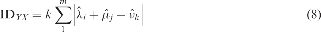
Multilevel studies of segregation have focused on using the variance as a measure of segregation from which the ID can be calculated. Intuitively this seems reasonable. Because the data are for places, the variance is measuring spatial variation (spatial heterogeneity) in the ethnic composition of neighbourhoods. Furthermore, the calculation of the ID, which, to recall, may be written as $k \sum_{i = 1}^{m} | ɛ_{i} |$ , is similar to the calculation of the total variance, which is $l \sum_{i = 1}^{m} ɛ_{i}^{2}$ , where l is the inverse of the degrees of freedom. Although the sum of squares is not the same as the sum of absolute values, typically the two are strongly correlated.

Figure 1 considers the relationship a little more. It shows the results of generating different values of the ID for two populations in 100, 150, 200, … 650, 700 neighbourhoods and then plotting the ID ( $k \sum_{i = 1}^{m} | ɛ_{i} |$ ) against the variance of the regression residuals ( $l \sum_{i = 1}^{m} ɛ_{i}^{2}$ ). Generally, the ID increases with the variance although not strictly linearly. The precise nature of the relationship varies with the number of neighbourhoods. Whereas the ID is constrained to lie within the range from 0 to 1, the variance is not and, at the extreme, different amounts of variance can all generate an ID score of one (this is not shown to avoid cluttering the graph). For example, a circumstance where population group X is found in only half the neighbourhoods, and group Y is only in the rest, has the same amount of segregation under the ID as a case where X is in 99% of the neighbourhoods and Y is in just the remaining 1. Under the variance measure these circumstances differ. Although the findings suggest that there is not a single formula that will link the variance to the ID, as an approximation the amount of the ID due to each level can be estimated as

{ID}_{(level)} ≅ {ICC}_{(level)} \times {ID}_{YX}

(10)

Figure 1.

The relationship between the variance of the regression residuals and the ID for n = 100, 150, 200, … , 650, 700 neighbourhoods.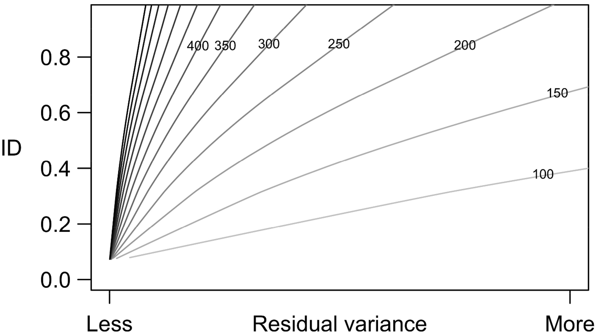

Using the ICC to measure spatial clustering

The key gain from the multilevel approach is that it addresses a well-known deficiency of the standard ID. As Duncan and Duncan (1955: 215) noted a half-century ago: “all of the segregation indexes have in common the assumption that segregation can be measured without regard to the spatial patterns of white and non-white residence in a city.”

The classic illustration of the problem is the checkerboard example shown in Figure 2. Each of the boards generates the same ID value of one even though the patterns of segregation, specifically the spatial clustering of the black and white populations, are not the same in each case.

Figure 2.

The Index of Dissimilarity cannot distinguish between these spatial patterns but the inter-class correlation can (cf. Table 1).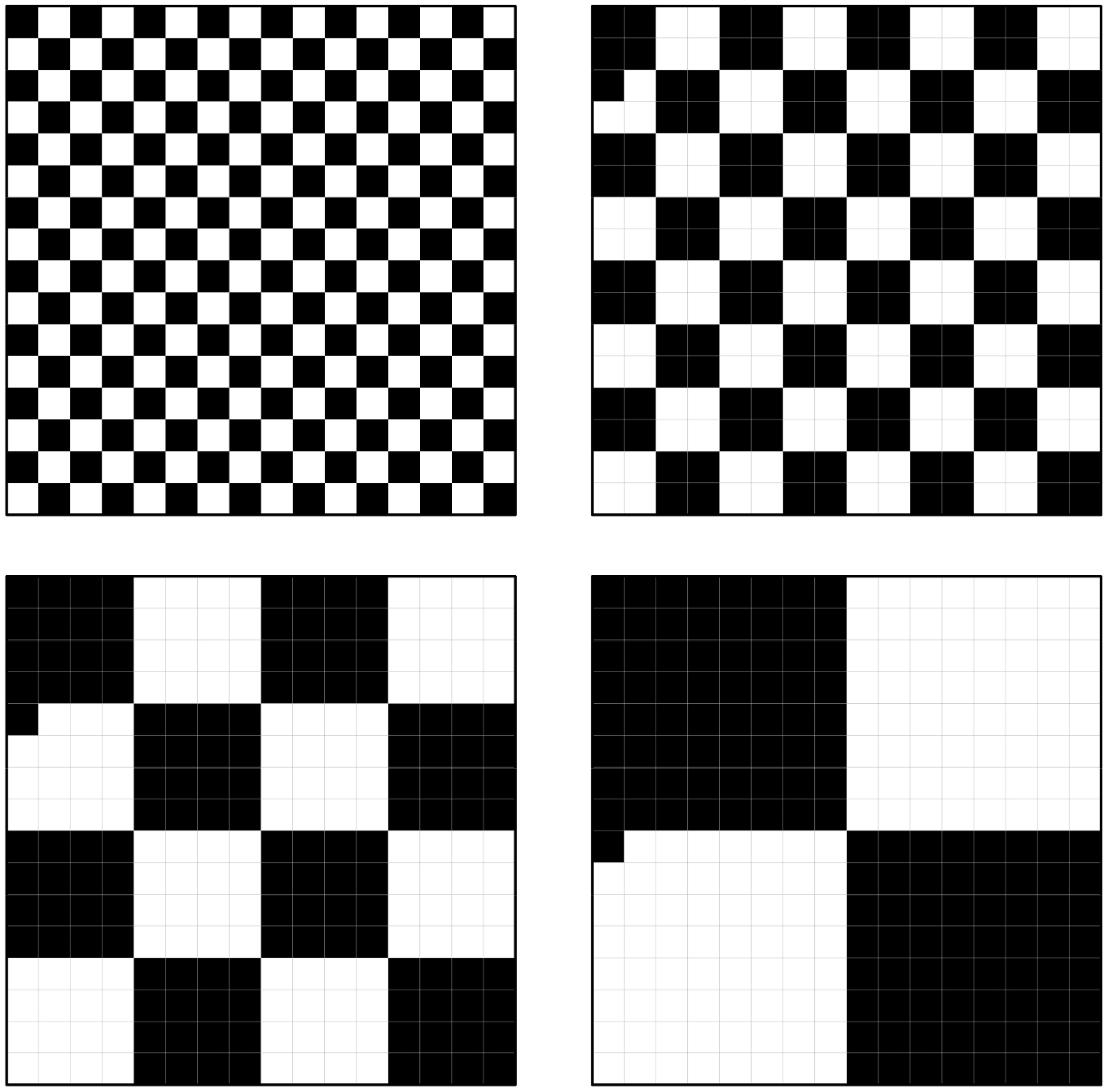

Although the ID cannot differentiate between them, the ICC can if the board is treated as a four-level model for which the individual squares at the base level are considered as part of a 2 by 2 grouping at level 2, a 4 by 4 grouping at level 3, and an 8 by 8 grouping at level 4. As Table 1 records, the ICC changes with the different patterns. Where the ID score is said to measure unevenness – the extent to which the relative distributions of the two populations match up across the study region – the ICC is measuring spatial clustering so the two principal dimensions of segregation are considered together.³

Table 1.

Showing the inter-class correlation for each of the examples in Figure 2.

	Proportion of the total variance
Level	Top-left	Top-right	Bottom-left	Bottom-right
1 by 1	1.000	0.156	0.156	0.156
2 by 2	0.000	0.984	0.000	0.000
4 by 4	0.000	0.000	0.984	0.000
8 by 8	0.000	0.000	0.000	0.984

The MLID package for R

Having set out the theory and what is measured, we now turn to its implementation in R. In much of its functionality, MLID it is an interface to the lme4 package for linear and generalised linear mixed-effects models in R, which is used to fit the models and from which the residuals at each level are extracted. The process of fitting the model is one of (1) loading the data table, (2) identifying which of its columns contain the counts of the population groups of interest, (3) specifying the geographic hierarchy, (4) fitting the model, (5) extracting the residuals, and (6) visualising the results. The impact of particular places and the consequences of omitting them from the model can be explored.

The data table, ethnicities, is bundled with the package and contains the population count for each of 181,408 small area Census OAs in England and Wales in 2011, cross-tabulated by ethnic group. It also records which of the 34,753 Lower Level Super Output Areas (LSOAs) the OAs belong to at a higher level of aggregation, which of the 7201 Middle Level Super Output Areas (MSOAs) at a level above that, which of the 348 Local Authority Districts (LADs) at the next level up and, finally, which of the 10 regions (RGNs). In 2011, the average area of an English or Welsh OA was approximately 0.76 km² (with an average population of 309 residents). For LSOAs it was 3.75 km² (with 1614 residents), for MSOAs, 18 km² (with 7787), LADs 375 km² (with 161,138) and for regions approximately 13,050 km² (with 5,607,591). On average, the ratio of the scales is approximately 1:5:25:495:17,200 (however, see the discussion in Section “Discussion and conclusion”).

Assuming the MLID package is installed, and taking as an example the residential segregation of the White British from the Bangladeshi population, then the standard ID is fitted by loading the package and data, and running the function,

> require(MLID)

> data(ethnicities)

> id(ethnicities, c("WhiteBrit", "Bangladeshi"))

Here, WhiteBrit and Bangladeshi are variable names in the ethnicities data frame.

Fitting the multilevel model differs only by specifying the levels. For a five-level model,

> id(ethnicities, c("WhiteBrit","Bangladeshi"), levels =

c("LSOA", "MSOA", "LAD", "RGN"))

for which the base level (the OAs) does not need to be specified because it corresponds to the rows of the data table. The ID is calculated, as are the ICC (shown as a percentage) and the holdback scores:

WhiteBrit ∼ Bangladeshi

ID: 0.852

Pvariance Holdback

Base 28.48 -12.16

LSOA 13.77 -3.14

MSOA 26.55 -4.66

LAD 26.82 -1.72

RGN 4.38 -12.32

The holdback scores calculate the percentage change in the ID if the effect at any one level is held back from the calculation, which is equivalent to setting the residuals for that level to zero. The difference between the ICC and the holdback scores is that the ICC assesses the relative size of the effect at each level whereas the latter assesses the overall impact of the effect upon the index. In the example above, the greatest proportions of the variance are at the OA, MSOA and LAD scales, at 0.285, 0.266 and 0.268, respectively. However, discounting the OA or regional effects has most impact on the ID, reducing it by 12.2 or by 12.3%. Although the regional effects are smallest in terms of the ICC their cumulative effect can be large because the calculation of the ID is additive (equation (8)) and regions contain many neighbourhoods.

Having fitted the model, the residuals at each level can be extracted and visualised using a caterpillar plot. This is a standard technique in multilevel modelling for which the residuals are ranked from highest to lowest and plotted on a chart together with their confidence intervals. The idea is to see whether at the tails of the distribution (the highest and least ranked values) any of the residuals differ statistically from zero or, alternatively, from other residuals.⁴ This amounts to asking whether there is any significant spatial variation between places at that level of the model. The output for the code below is shown in Figure 3.

> model1 <- id(ethnicities, c("WhiteBrit","Bangladeshi"),

Figure 3.

Caterpillar plots showing the residual differences – the differences between the shares of the White British population and the shares of the Bangladeshi population – at the higher levels of the model.

levels = c("LSOA", "MSOA", "LAD", "RGN"))

> ci <- confint(model1)

> catplot(ci)

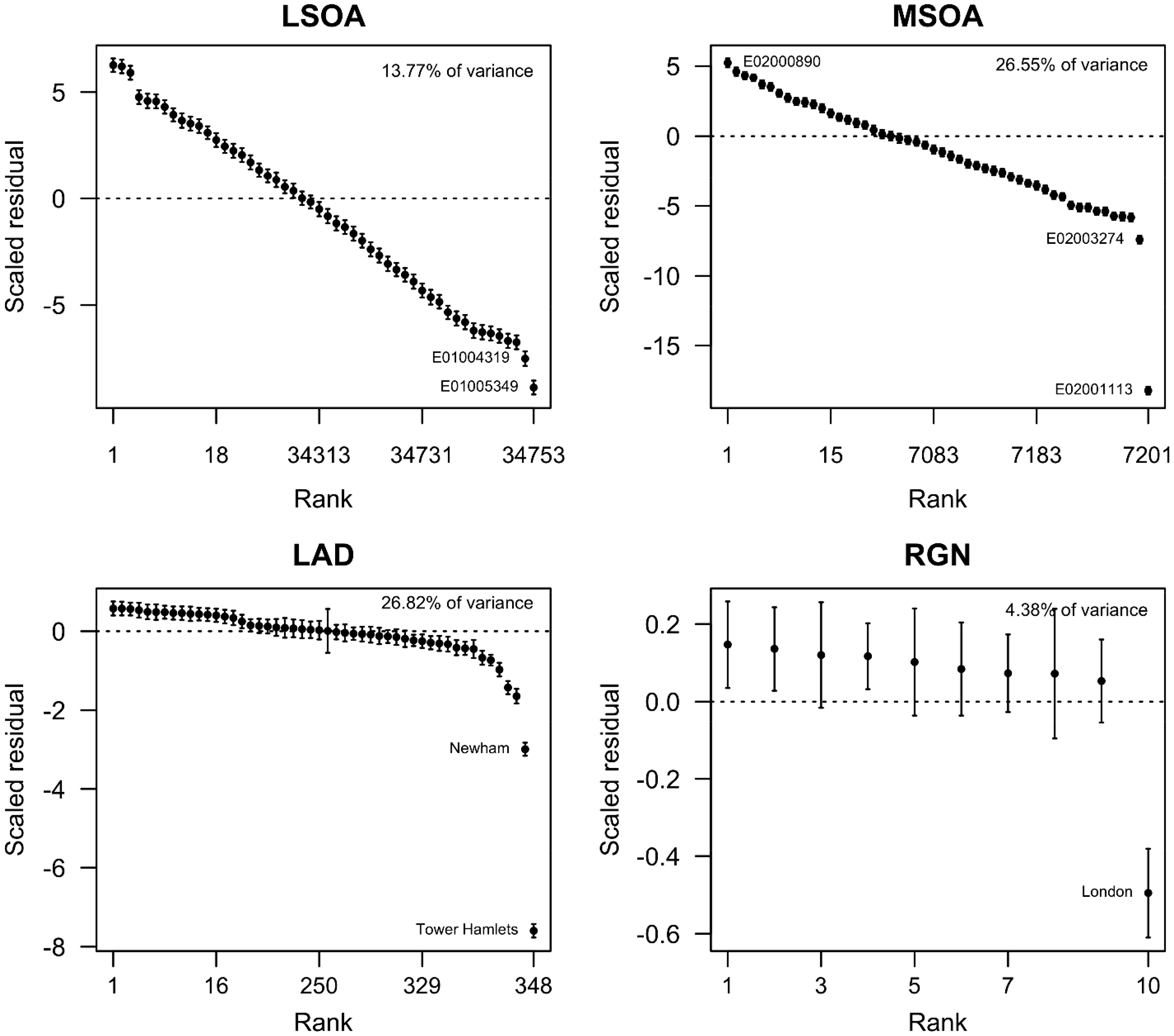
Looking at Figure 3, it can be seen that the London Borough of Tower Hamlets, within London’s former docklands, has a share of the White British population that is much less than its share of the Bangladeshi population, and that difference is much greater than for other local authorities. The same is true of London as a whole. The size of the London effect (the residual) is less but given the size of London and the number of neighbourhoods it contains it is sufficient to have a high impact on the ID score, which is what the holdback scores showed.

The package allows for the impact of particular places upon the ID to be assessed. For example,

> effect(model1, "Tower Hamlets")

reveals that Tower Hamlets accounts for almost half the variation in the difference in share between the White British and Bangladeshi populations across all neighbourhoods in England and Wales, and that Tower Hamlets’ neighbourhoods contribute to almost 11% of the total ID, which is about 25 times more than expected given how many of the total number of English and Welsh neighbourhoods are in Tower Hamlets. Omitting Tower Hamlets from the data more than halves the local authority effect in respect to the ICC, which is unsurprising given that almost 20% of the entire Bangladeshi population of England and Wales lived in Tower Hamlets in 2011.

Finally, because each residual refers to a location, they can be mapped with the addition of a suitable boundary file. How to visualise this effectively is a challenge because of the number and small sizes of the areas used at the base level. One way is to employ kernel density estimation, here using R’s spatstat package for spatial point pattern analysis. The idea is at each location (the centroid of each OA), the effect of any one level in the model – the local authority, for example – acts to raise or to attenuate the index value; that is, to increase or decrease the value of $| ɛ_{i} |$ . A density surface can be created mapping the density of points where the local authority effect leads to an increase in the measured segregation, which is then divided by a corresponding surface mapping the density of all points in the study region to control for the geography of the neighbourhoods. The result is to produce a map indicating where the local authority scale is associated with the pattern of segregation.

Figure 4 takes this approach and applies it to the White British and Bangladeshi segregation in 2011, showing the results at the OA and LAD scales for London. What it reveals is a spatial structure. Local level, OA patterns of difference matter more on the outskirts of London, particularly in the South East. Broader scale, local authority patterns matter most in the North East, in and around the Docklands region. We comment more on the non-stationarity of the effects in Section “Discussion and conclusion”.

Figure 4.

Mapping the scales of White British – Bangladeshi residential segregation in London in 2011. Darker shading indicates the places where (a) the OA, or (b) local authority effects act to increase the measured amount of segregation.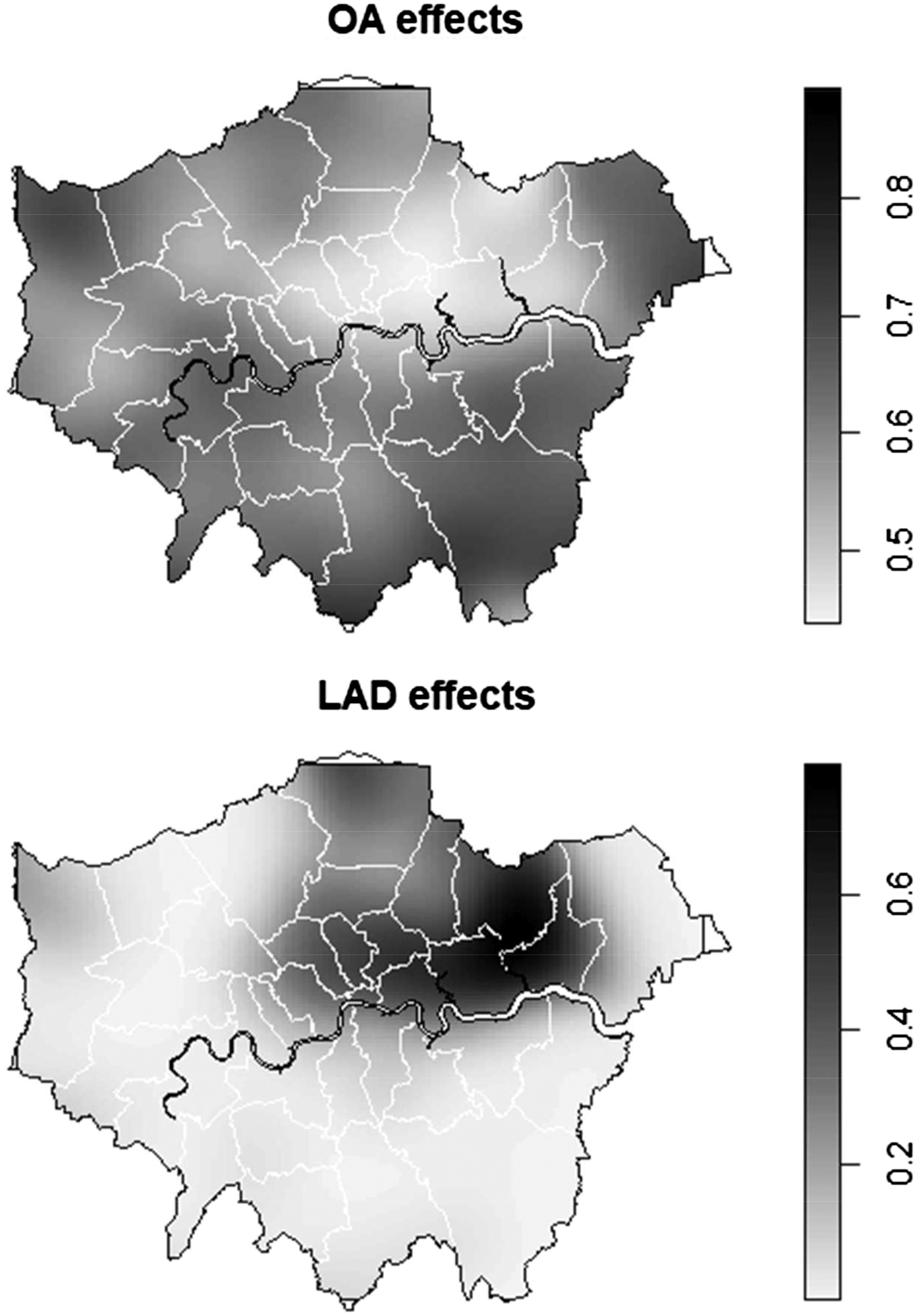

The changing scales of residential ethnic segregation in England and Wales

The White British – Bangladeshi segregation examined in the preceding section was the highest between any of the major ethnic groups enumerated in the 2011 Census. Even so, its ID value of 0.852 was lower than it had been in 2001 when it was 0.907. Those values are shown in Table 2. The upper triangle of the matrix contains the scores for 2001, the lower contains those for 2011. In the main, the groups are the same as those used in the Census except that we have combined the various mixed ethnicity groups, as well as the white but not White British groups, and omitted some of the smaller “other ethnicity” groups such as Other Black and Other Asian. In all but one case a decrease in segregation is recorded. The exception is the White British from other white groups. That rose from 0.457 to 0.496 but remains relatively low when compared to the values for other groups.

Table 2.

Showing the pairwise ID scores based on the residential counts of nine ethnic groups present in the 2001 and 2011 Census counts for England and Wales. The diagonal records the averages; the values in parentheses are the group’s percentage of the total population that year. (WhBrit: White British; Bang: Bangladeshi; Indian: Indian; Pak: Pakistani; BlAf: Black African; BlCar: Black Caribbean; Chinese: Chinese; WhOth: White Other; Mixed: mixed ethnicity).

	2001 ID score (and % of the population)
2011 ID score (and % of the population)		WhBrit (88.4)	Bang (0.55)	Indian (2.01)	Pak (1.39)	BlAf (0.93)	BlCar (1.10)	Chinese (0.44)	WhOth (3.86)	Mixed (1.28)
	WhBrit (83.1)	0.726 0.688	0.907	0.728	0.826	0.823	0.770	0.779	0.457	0.520
	Bang (0.82)	0.852	0.797 0.746	0.806	0.749	0.745	0.753	0.835	0.803	0.782
	Indian (2.60)	0.700	0.743	0.694 0.649	0.665	0.709	0.647	0.745	0.628	0.628
	Pak (2.07)	0.812	0.691	0.630	0.756 0.717	0.783	0.711	0.837	0.761	0.718
	BlAf (1.82)	0.742	0.704	0.652	0.719	0.684 0.617	0.469	0.717	0.619	0.606
	BlCar (1.09)	0.756	0.721	0.639	0.694	0.441	0.653 0.625	0.741	0.600	0.530
	Chinese (0.72)	0.670	0.790	0.675	0.787	0.650	0.700	0.744 0.672	0.633	0.663
	WhOth (5.55)	0.496	0.739	0.580	0.720	0.536	0.561	0.539	0.616 0.565	0.430
	Mixed (2.25)	0.474	0.724	0.572	0.685	0.493	0.489	0.562	0.347	0.610 0.543

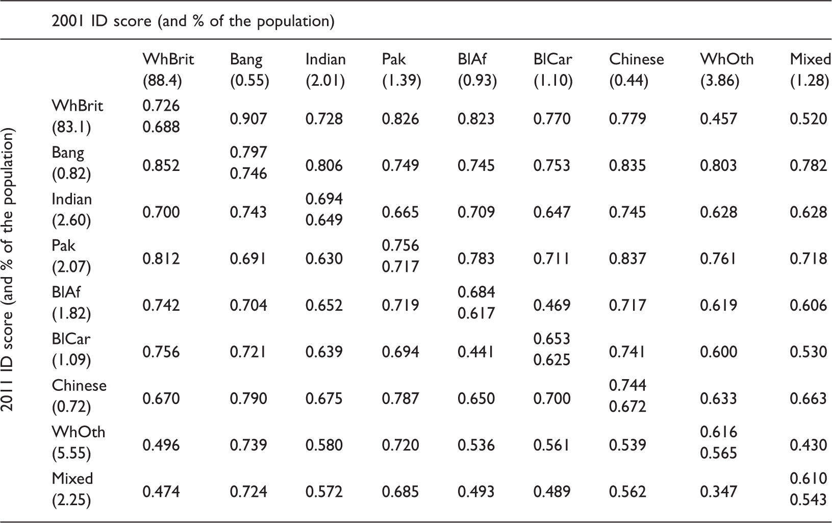
ID: Index of Dissimilarity.

The diagonal of the matrix is the average of the scores for each ethnic group in 2001 and in 2011. On the basis of the average, the Bangladeshi group was the most segregated in both 2001 and 2011, the Pakistani group second most, and those of a mixed (joint) ethnicity least. This does not mean that the Bangladeshis nor any of the other groups are choosing to self-segregate, nor that the segregation is voluntary because the raw figures say nothing about causes. It should be remembered that the ID is a relative measure: it compares the geographical distribution of one group with another to measure their unevenness with respect to each other. Therefore, the very high segregation between the Bangladeshis and the White British in both 2001 and 2011 can be due to the residential choices/constraints of the White British or the Bangladeshis, or both.

For the Pakistanis, Black Africans and Black Caribbeans, as well as for the Bangladeshis, it is segregation from the White British that generates some of the highest scores in Table 2. Explanations include the co-occurrence of economic and ethnic segregation that minority groups disproportionately encounter (Harris et al., 2017) which limits their residential choices, as well as the White British’s much greater prevalence in suburban and rural areas, outside of the cities where other groups are concentrated. The results confirm what other authors have shown: ethnic, residential segregation decreased in England and Wales over the intercensal period from 2001 to 2011 (Catney, 2016a, 2016b; Harris, 2014; Johnston et al., 2013). Over that decade all groups except the White British increased in size (the number of White British decreased marginally, by 0.876%). As the groups have grown their segregation has decreased.

Figure 5 turns to the primary area of interest: the results of refitting the indices as a five-level multilevel model in which the counts by OA are nested into LSOAs, MSOA, LADs and Regions at the higher levels. Recall that calculating the ID in this way does not alter the overall index values but it does allow for the geographic scales of the segregation patterns (the spatial clustering) to be investigated with consideration to the residual variance, the ICC and the decomposition of the ID by each level of the model.

Figure 5.

Decomposing the ID by the levels of the model in 2001 and 2011 for the most segregated pairs of ethnic groups.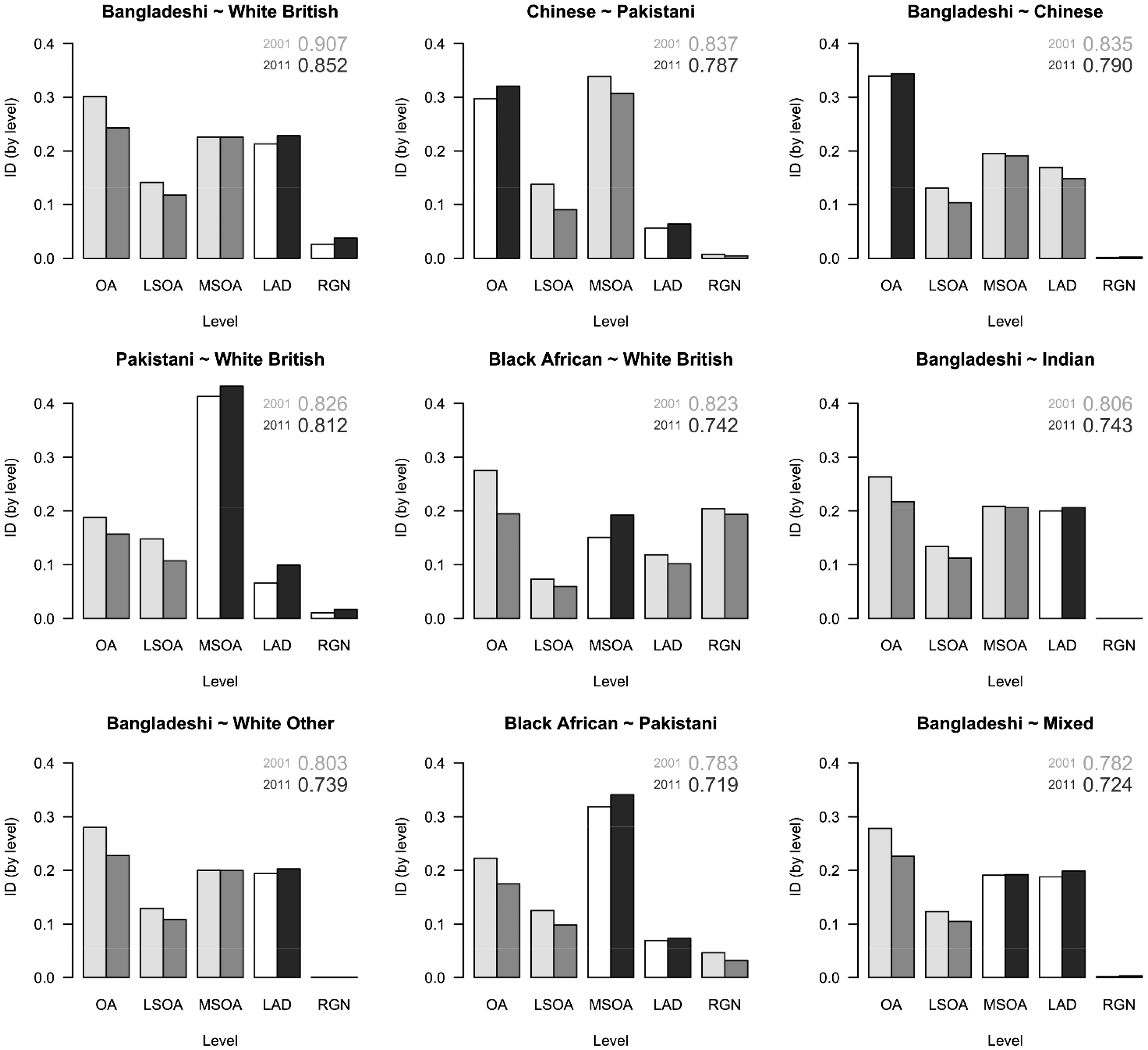

Figure 5 shows the results of applying the decomposition to the nine most segregated pairs of ethnicities in 2001 (the nine highest values in the top triangle of Table 2) to consider how the amount and geographic scale of their segregation changes to 2011. The height of each column is the part of the total ID due to each level (from equation (10)) with the sum across the columns for any year equal to the overall ID score. The values for 2001 are shaded lighter than those for 2011, with the darkest shading applied to highlight cases where the ID for that level increased over the period.

In six of the nine cases it the smallest area scale, the OAs, that contribute most to the patterns of segregation in 2001. The three exceptions all include the Pakistani group where a greater part of the segregation is at the more aggregate MSOA scale. A reason may be that the patterns of residential clustering map more closely to the MSOA scale for the Pakistanis than they do for the others. By 2011, the OAs still contribute most but generally the biggest falls have occurred at this scale; for example, the decrease is from 0.30 to 0.24 for the separation of the Bangladeshi and White British populations.

Again, there are exceptions, both of which include the Chinese group: the OA level values rise from 2001 to 2011 for the Chinese–Pakistani and Bangladeshi–Chinese segregation. Nevertheless, what appears to be happening overall is an upscaling of the patterns of segregation from the lower level geographies, the OAs and the LSOAs, to the higher-level ones, the MSOAs and LADs. When the analysis is extended to include all the pairwise comparisons, there is found to be a reduction in the average variance at the OA and LSOA scales, and an increase at the MSOA and LAD scales for all groups except the Chinese.

Here, we encounter a problem in interpreting a multilevel index because a shift in the pattern of segregation from the small areas to coarser scales is not necessarily evidence of more ethnically mixed neighbourhoods. Returning to the example of a checkerboard and imagining that the black squares represent the residential locations of a minority group, it may be that as the group grows and spreads outwards so some of the surrounding squares change from white to black (or, at least, a shade of grey). That represents an increase in the scale of clustering but also a process of deconcentration and spreading out, correctly associated with a pattern of decreasing segregation.

However, there is a competing explanation. Imagine a process whereby the pattern shown in the top-left of Figure 2 changes to one of the more clustered patterns of segregation shown in the rest of the same graphic. The consequence would be that the average residential distance between the “black” and white populations increases. If so, then an upscaling in the geographic scale of segregation is also an upscaling in their degree of separation.

So which process applies to the changes occurring in England and Wales: a process of agglomeration or a process of dispersion? The multilevel approach provides no immediate answer although a process of agglomeration assumes that the two groups were well spread across the board in the first place, which they were not. A truer representation of the residential geography of England and Wales would see most of the board shaded white (for White British) with far fewer of the other squares representing the residential locations of other ethnic groups.

Furthermore, we know that the overall segregation scores are declining. As an additional piece of information, we have identified the OAs that in 2001 or 2011 contained at least eight persons from six or more of the eight ethnic groups that remain having omitted the White other category because it includes most of the (politically contentious) immigration from the expansion of the EU into Eastern Europe from 1 May 2004 and therefore measures something rather different in 2011 than it did in 2001.

Although the threshold of eight persons is somewhat arbitrary – but not entirely so, it was chosen as an amount that typically would require at least two households to be resident –, the message is clear: the percentage of Bangladeshis living in these ethnically diverse neighbourhoods increased from 31.0 to 40.8 over the decade; for Indians, from 21.2 to 27.1%; for Pakistanis, from 22.6 to 33.1; for Black Africans from 25.7 to 30.7; and for Black Caribbeans, from 16.9 to 34.0%. Only for the Chinese did the percentage fall, from 23.8 to 22.2%. This fits with the findings of Johnston et al. (2014) who identify a process of dispersion and spatial diffusion for minority groups across cities in England and Wales as their numbers grow and as they move out from their previous enclaves.

For the White British, the percentage is unchanged at 2.8 but that stability disguises a slight increase in the percentage living in neighbourhoods where none but the White British were present under the eight persons criterion: an increase from 59.6 to 62.3%. Whilst minority groups have spread outward there has been a degree of spatial contraction by the White British from large cities. Even so, in terms of the residential locations of most ethnic groups, segregation has decreased over the decade and so it would be hard to sustain the argument that minority groups are choosing to live in segregated neighbours (see also Finney and Simpson, 2009).

Discussion and conclusion

This paper has outlined the basis for a MLID and discussed its implementation in R. The advantages of the approach have been identified as usability, reproducibility and computational speed, and as a method of measuring the two principal dimensions of segregation simultaneously, which are distributional unevenness and spatial clustering.

However, neither this nor other multilevel approaches are without limitation. A first is not a problem with the method as such but its application to administrative data linked to zones of varying shape and size. In England and Wales, census areas vary markedly in size: from approximately 0.03 to 1.01 km² from the first to the ninth decile for OAs; from 0.13 to 8.33 km² for LSOAs; from 0.75 to 54 km² for MSOAs; from 27 to 904 km² for LADs; and from 1416 to 19,600 km² for Regions. There is not a one-to-one relationship between the levels of the model and the geographic scale of analysis they represent.

A solution may be to use standardised and regularised grid geographies (https://popchange.liverpool.ac.uk/, Dmowska and Stepinski, 2014) which can be aggregated into larger grid cells, at coarser scales, in the same way that the multilevel approach was applied to Figure 2 to differentiate the four scales of clustering. However, what that demonstration did not reveal is that the results are dependent upon which is chosen to be the starting cell of the aggregation process (the corner of the aggregated grid). The results will reflect that decision.⁵

A second problem is the interpretation of the variance measures and the ICC. The ICC, like the overall ID value, is a general measure of segregation, a global statistic, that can hide spatial heterogeneity. Consider the example given in Section “The MLID package for R” looking at the residential segregation of the White British from the Bangladeshi population. That revealed much of the variance (26.8%) to be at the LAD level, suggesting geographical differences between places at that scale. The complication is that the value is itself geographically non-stationary: the LAD level share of the variance is as high as 54.10% for London and as low as 2.21% in the North East of England. At the base level, OA level differences account for 69.92% of the variance in the South West but only 22.81 in London. In-between, the importance of the intermediate levels varies from place to place, both between and within regions. The spatial scales of segregation vary spatially.

A third problem, specific to the MLID, is the handling of stochastic effects. It is not clear how the methods used by Jones et al. (2015), amongst others, can be applied because theirs are based on population counts and not on shares of a group’s total (it is, however, still possible to estimate the expected ID under randomisation: Harris, 2017a). A pragmatic response is to recognise that a high value under randomisation arises when trying to conduct analysis at a scale for which there is insufficient data because of the relative scarcity of a population group. It may be better in such circumstances simply to aggregate the data to a different base scale or to apply weightings to the calculations in accordance with the population size.

A final problem was suggested in the case study – the models measure outcomes not processes. Comparing models and looking at change can be suggestive: here, the decrease in the numeric but increase in the geographic scale of segregation suggests a process by which minority groups are spreading out. However, correspondence between patterns and processes is inexact and the models do not answer the more fundamental questions: what are the causes of segregation, do they matter, and if so for whom and why? These questions are topical in the UK where the Prime Minister has launched an “inequality audit” and an associated website to explore ethnic inequalities across multiple dimensions of the life course.⁶

Nevertheless, empirical evidence does set the context for discussion and debate, and that is important in a world of conflicting “truths” not all of which are equally valid or verified. Measures of segregation may not provide all the answers but they do provide the information to identify a problem or to challenge misperception. In the UK, the idea that ethnic segregation is increasing persists in media and political discourse and is used to frame policies that tend to be directed at and carry expectations of the behaviours and choices of minority groups. However, evidence from the census shows the opposite to be true: residential segregation has decreased over the decade to 2011 with minority groups living in more mixed neighbourhoods.

Of course, it is possible that desegregation has subsequently reversed but at the current time there is not the data to show it. Most likely there are parts of the country where segregation persists or has increased due to local circumstances, including the demographic (e.g. age and fecundity of the population). However, as Burgess and Harris (2017) note in relation to discussions of school-level segregation in England and Wales, “we need to be careful about drawing attention to and making policy based on any exception to a general rule. We will always find places where segregation is increasing though usually only in the short-term due to demographic changes. But if the overall trend is one of decreasing segregation – however measured – then that is the key result that needs to be emphasised.” The MLID can help support that emphasis whilst remaining cognisant of spatial variation, identifying both the exceptions and the norm.

Footnotes

Acknowledgements

My grateful thanks for the comments of the referees for improving the clarity of the work.

Declaration of conflicting interests

The author(s) declared the following potential conflicts of interest with respect to the research, authorship, and/or publication of this article: Richard Harris is an editor of this journal.

Funding

The author(s) disclosed receipt of the following financial support for the research, authorship, and/or publication of this article: The research was funded under the Economic and Social Research Council’s (ESRC) Urban Big Data Centre (), ES/L011921/1.

Notes

Richard Harris is Professor of Quantitative Social Geography at the University of Bristol.

Dewi Owen was a postgraduate at the School of Geographical Sciences, University of Bristol where he studied multilevel models of segregation.

References

Bates

Maechler

Bolker

et al. (2015) Fitting linear mixed-effects models using lme4. Journal of Statistical Software 67: 1–48.

Brunsdon

(2016) Quantitative methods. I. Reproducible research and quantitative geography. Progress in Human Geography 40: 687–696.

Burgess S and Harris R (2017) (Mis-)understanding school segregation in England? Comments on a new measure of segregation. Available at: http://simonburgesseconomics.co.uk/blog/ (accessed 16 May 2017).

Casey

(2016) The Casey Review: A Review into Opportunity and Integration, London: Department for Communities and Local Government.

Catney

(2016a) Exploring a decade of small area ethnic (de-)segregation in England and Wales. Urban Studies 5: 1691–1709.

Catney

(2016b) The changing geographies of ethnic diversity in England and Wales, 1991–2011. Population, Space and Place 22: 750–765.

Dmowska

Stepinski

(2014) High resolution dasymetric model of U.S. demographies with application to spatial distribution of racial diversity. Applied Geography 53: 417–426.

Duncan

(1955) A methodological analysis of segregation indices. American Sociological Review 20: 210–217.

Finney

Simpson

(2009) ‘Sleepwalking to Segregation’? Challenging Myths about Race and Migration, Bristol: Policy Press.

10.

Gorard S and Taylor C (2002) A Comparison of Segregation Indices in Terms of Strong and Weak Compositional Invariance. Sociology 36: 875–895.

11.

Harris

(2014) Measuring changing ethnic separations in England: A spatial discontinuity approach. Environment and Planning A 46: 2243–2261.

12.

Harris

(2017a) Measuring the scales of segregation: Looking at the residential separation of White British and other schoolchildren in England using a multilevel index of dissimilarity. Transactions of the Institute of British Geographers. DOI: 10.1111/tran.12181.

13.

Harris R (2017b) MLID: Tools and Functions to Fit a Multilevel Index of Dissimilarity. School of Geographical Sciences, University of Bristol. Available at: https://cran.r-project.org/web/packages/MLID/ (accessed 16 May 2017).

14.

Harris

Johnston

Manley

(2017) The changing interaction of ethnic and socio-economic segregation in England and Wales, 1991–2011. Ethnicities 17(3): 320–349.

15.

Hong S-Y, O’Sullivan D and Sadahiro Y (2014) Implementing spatial segregation measures in R. PLoS ONE. 9(11): e113767.

16.

Hongwei

Logan

Short

(2014) Integrating space with place in health research: A multilevel spatial investigation using child mortality in 1880 Newark, New Jersey. Demography 51: 811–834.

17.

Johnston

Poulsen

Forrest

(2013) Multiethnic residential areas in a multiethnic country? A decade of major change in England and Wales. Environment and Planning A 45: 753–759.

18.

Johnston

Poulsen

Forrest

(2014) Increasing diversity within increasing diversity: The changing ethnic composition of London’s neighbourhoods 2001–2011. Population Space and Place 21: 38–53.

19.

Jones

Johnston

Manley

et al. (2015) Ethnic residential segregation: A multilevel multigroup multiscale approach exemplified by London in 2011. Demography 52: 1995–2019.

20.

Leckie

Goldstein

(2015) A multilevel modelling approach to measuring changing patterns of ethnic composition and segregation among London secondary schools 2001–2010. Journal of the Royal Statistical Society Series A 178: 405–424.

21.

Leckie

Pillinger

Jones

et al. (2012) Multilevel modelling of social segregation. Journal of Educational and Behavioral Statistics 37: 3–30.

22.

Lee

Reardon

Firebaugh

et al. (2008) Beyond the census tract: Patterns and determinants of racial segregation at multiple geographical scales. American Sociological Review 73: 761–791.

23.

Manley

Johnston

Jones

et al. (2015) Macro-, meso- and microscale segregation: Modeling changing ethnic residential patterns in Auckland New Zealand 2001–2013. Annals of the Association of American Geographers 105: 951–967.

24.

Morrill

(1991) On the measure of geographic segregation. Geography Research Forum 11: 25–36.

25.

Östh

Malmberg

Andersson

(2014) Analysing segregation with individualized neighbourhoods defined by population size. In: Lloyd

Shuttleworth

Wong

(eds) Social-Spatial Segregation: Concepts, Processes and Outcomes, Bristol: Policy Press.

26.

Owen D (2015) Measuring residential segregation in England and Wales: A model-based approach. Unpublished PhD Thesis, School of Geographical Sciences, University of Bristol.

27.

Powell MJD (2009) The BOBYQA Algorithm for Bound Constrained Optimization without Derivatives. Department of Applied Mathematics and Theoretical Physics, Cambridge University. Available at: www.damtp.cam.ac.uk/user/na/NA_papers/NA2009_06.pdf (accessed 16 May 2017).

28.

Reardon

Farrell

Matthews

et al. (2009) Race and space in the 1990s: Changes in the geographic scale of racial residential segregation 1990–2000. Social Science Research 38: 55–70.

29.

Reardon

Matthews

O’Sullivan

et al. (2008) The geographic scale of metropolitan segregation. Demography 45: 489–514.

30.

Reardon

O’Sullivan

(2004) Measures of spatial segregation. Sociological Methodology 34: 121–162.

31.

Reardon

Yun

McNulty

(2000) The changing structure of school segregation: Measurement and evidence of multiracial metropolitan-area school segregation, 1989–1995. Demography 37: 351–364.

32.

Spielman

Logan

(2013) Using high-resolution population data to identify neighbourhoods and establish their boundaries. Annals of the Association of American Geographers 103: 67–84.

33.

Theil

(1972) Statistical Decomposition Analysis, Amsterdam: North-Holland.

34.

van Belle

(2008) Statistical Rules of Thumb, 2nd ed. New York: Wiley.

35.

Wong

D W S

(1993) Spatial indices of segregation. Urban Studies 30: 559–572.

Implementing a Multilevel Index of Dissimilarity in R with a case study of the changing scales of residential ethnic segregation in England and Wales

Abstract

Keywords

Introduction

Multilevel modelling of segregation: An overview

MLID: Statistical basis and concept

Forming the index within a regression framework

The relationship between variance and the ID

Using the ICC to measure spatial clustering

The MLID package for R

The changing scales of residential ethnic segregation in England and Wales

Discussion and conclusion

Footnotes

Acknowledgements

Declaration of conflicting interests

Funding

Notes

References