
Abstract
The authors present a straightforward method for assessing symmetry and asymmetry in the effect of an independent variable, on the basis of its direction of change, on a dependent variable in statistical models and provide two different empirical illustrations: (1) the effect of economic change on electricity production in nations and (2) the effect of change in income on wealth accumulation among individuals. In so doing, the authors also demonstrate specific ways to illustrate and interpret asymmetrical effects. Finally, the authors note a variety of theoretical reasons to expect asymmetry and suggest areas in which it may be observed.
Thirty years ago, Stanley Lieberson (1985) argued for the importance of recognizing asymmetrical forms of causation, with respect to the effects of different directions of change of an independent variable on a dependent variable, in the social sciences. However, to this day, virtually no statistical analyses in sociology assess whether effects are asymmetrical, implicitly assuming they are symmetrical. In a symmetrical relationship, the independent variable has the same magnitude of effect on the dependent variable regardless of whether the independent variable is increasing or decreasing. In an asymmetrical relationship, the independent variable has a different magnitude of effect when it is growing than when it is declining. For example, a standard symmetrical model would predict the price of gas relative to a particular price of oil to be the same regardless of whether the oil price increased or decreased to its value. However, as most drivers have probably experienced, gas prices “correct” to increases in the price of oil more readily than they do to declines in the price of oil (Radchenko 2005).
The symmetrical or asymmetrical character of any relationship is a fundamental issue and is different from recursive or nonrecursive and linear or nonlinear distinctions. Recognizing the difference between asymmetrical and symmetrical relationships is not only a technical consideration for statistical analyses but has important implications for developing and testing theories and designing public policies. As Lieberson (1985) explained, reversibility is a ubiquitous principle in most social research. Researchers and policy analysts alike typically (usually implicitly) assume symmetrical causation. This assumption may result in unrealistic expectations about results and, perhaps more important, about policies. If a causal process is not reversible or if eliminating a cause does not remove the consequence of a prior causal process, then social policies based on reversibility are bound to fail. Lieberson argued that sociology will be “inescapably marred” (p. 73) if we continue to ignore this distinction. Yet with a few typically conceptual exceptions, sociology has not heeded this warning.
To facilitate incorporation of the distinction between symmetrical and asymmetrical processes into sociological theory and analysis, we present a straightforward method for assessing whether the relationship between two variables is asymmetrical or symmetrical. To illustrate this technique, we present two analyses, one of the effect of gross domestic product (GDP) on electricity production in nations and the other of the effect of income on wealth accumulation among individuals in the United States. We also demonstrate specific novel ways to interpret and present asymmetrical relationships.
The Distinction between Symmetrical and Asymmetrical Processes
To avoid confusion, it is important to note that causal relationships 1 may be symmetrical or asymmetrical in a variety of ways (Hausman 1998), and here we are only considering symmetry and asymmetry with respect to the direction of change (increase vs. decrease) in an independent variable, what we here refer to as directional symmetry or asymmetry. Commonly, references to the asymmetry of a causal process refer to temporal asymmetry (i.e., the understanding that causes precede effects in time). Closely related to the issue of temporal order is the basic distinction about the asymmetry between cause and effect, whereby changes in factor A (the cause) lead to changes in factor B (the effect), but changes in B do not lead to changes in A. 2 This type of asymmetry relates to direction of flow of causality (A to B vs. B to A), which in principle can be sorted out with temporal order. Symmetry and asymmetry of this nature and of other types (see Hausman 1998) are distinct from asymmetry of effect related to the direction of change in an independent variable, which is our interest here.
In the standard type of regression model used in sociology, the value of a dependent variable, y, is predicted on the basis of the value(s) of one or more independent variables, xk. In this type of model, the history of changes in the independent variable(s) is not taken into account in the estimated effects. That is to say, whether an independent variable increased to its observed value or decreased to its observed value is not reflected in the model. Even in panel and time-series models, the direction of change of the independent variables does not affect the predicted y value; that is, a given value of x predicts a particular value of y (in combination with other factors in the model), regardless of whether x increased or decreased to reach its observed value.
The nature of asymmetry in linear and nonlinear relationships is illustrated in Figure 1. Because with asymmetrical relationships the predicted value of y for a given value of x depends on the history of change in x, there is not a singular way to graph y versus x. Therefore, we make the graph on the basis of a particular scenario. In Figure 1A, the relationship between x and y is linear and asymmetrical, whereby a one-unit increase in x leads to a two-unit increase in y, but a one-unit decrease in x leads to only a one-unit decrease in y. In this scenario, x increases one unit at each point in time from T1 through T10, then x decreases one unit for each point in time from T10 to T19, returning x to its starting value. As the graph shows, the curve for when x is decreasing is different for the curve when x is increasing, and even though x returns to its original value, y does not return to its starting value. In Figure 1B, the relationship between x and y is nonlinear and asymmetrical, whereby a one-unit increase in x leads to a 20 percent increase in y, but a one-unit decrease in x leads to only a 10 percent decrease in y (this type of relationship could be modeled by regressing the logarithm of y on x). As in Figure 1A, the curve for when x is increasing is different from when x is decreasing, but both curves are nonlinear. For both Figures 1A and 1B, if the relationships were symmetrical, the curve for T1 to T10 would be identical to the curve for T10 to T19. The gap between the curve for T1 to T10 and the curve for T10 to T19 reflects the degree of asymmetry.

Linear and nonlinear asymmetrical relationships. Each panel presents a hypothetical, abstracted relationship between x and y. In panel A, the relationship is linear, such that a one-unit increase in x leads to a two-unit increase in y, but a one-unit decrease in x leads to a decrease in y of only one unit. Panel B presents a nonlinear relationship, whereby a one-unit increase in x leads to a 20 percent increase in y, but a one-unit decrease in x leads to a decrease in y of only 10 percent. Both panels present a scenario in which x increases by one unit between each increment of time from T1 to T10 and then decreases by one unit between each point from T10 to T19. The solid lines show the curve when x is increasing, and the dashed lines show the curve when x is decreasing.
Asymmetrical relationships can lead to a ratcheting effect, as illustrated in Figure 2. In the scenario presented here, x oscillates between a value of 10 and 11, and the relationship between x and y is one in which a one-unit increase in x leads to a two-unit increase in y, but a one-unit decrease in x leads to only a one-unit decrease in y. Even though at time 5, x has the same value it had at time 1, y has increased from 10 to 12, showing that the effect of x is partially irreversible. Note that, of course, it could alternatively be the case that a decrease in x leads to a bigger decrease in y than an increase in x leads to an increase in y, in which case there would be a ratcheting down instead of a ratcheting up. Also, of course, an asymmetrical relationship between x and y could be negative and asymmetrical, whereby an increase in x leads to a decrease in y and a decrease in x leads to an increase in y, but these effects are different from one another in magnitude.
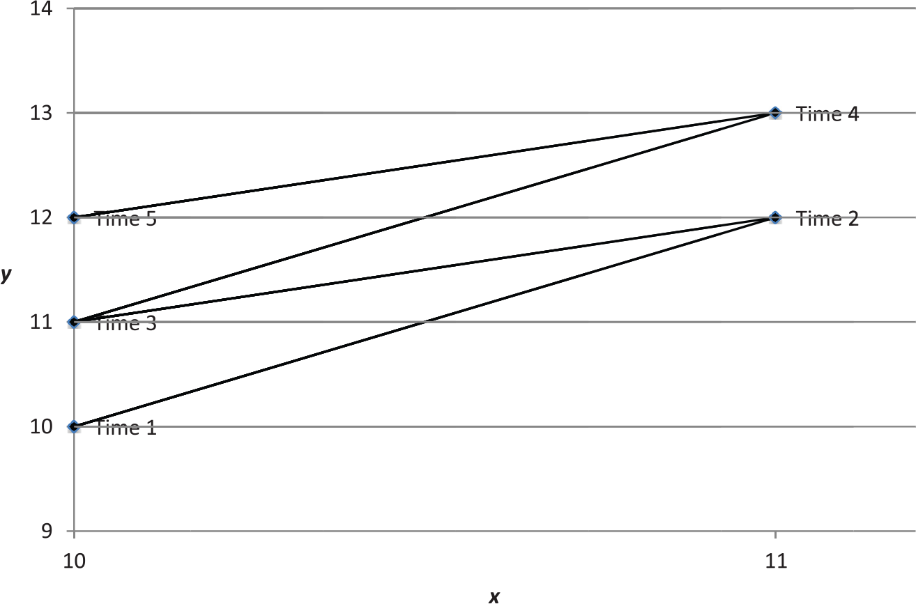
Asymmetry ratcheting effect. The figure illustrates the ratcheting effect from a hypothetical, abstracted asymmetrical relationship between x and y, whereby an increase in x of one unit leads to an increase in y of two units, but a decrease in x of one unit leads to a decrease in y of only one unit. The value of x oscillates between 10 (times 1, 3, and 5) and 11 (times 2 and 4).
The issue of asymmetry has received some social scientific attention but by and large has been neglected despite its important theoretical, substantive, and policy implications. Although this general neglect is pronounced, several areas of research have addressed some aspect of this issue. For example, economists have modeled a variety of asymmetrical processes, such as those related to gross national product (Brunner 1997), monetary shocks (Thoma 1994), price changes (Peltzman 2000), including the aforementioned case of gas and oil prices (Radchenko 2005) and the effect of prices and income on energy and oil demand (Gately and Huntington 2002). 3 Criminological research has considered direction of change in variables sporadically and with mixed results (see Cohen, Felson, and Land 1980; LaFree and Drass 1996), as have some analyses in political science (Clark, Gilligan, and Golder 2006). Research on the sociology of health suggests that tipping points might reduce the likelihood of reversibility in medical outcomes, but this is largely conceptual work (see Williams 1990). Similarly, demographic research offers conceptual justifications for asymmetrical effects in fertility and development (see Morgan and Taylor 2006), and research on social networks has used asymmetry to discuss differences between tie formation and tie retention (Habinek, Martin, and Zablocki 2015). However, to our knowledge, there is no clear presentation in the sociological literature of appropriate general methods for assessing, presenting, and interpreting asymmetrical relationships, which is what we aim to provide.
Assessing Asymmetrical Effects
Here, we explain a statistical strategy for estimating asymmetrical effects, and we illustrate this approach by examining two different relationships. First, we look at the effects of economic growth and decline on electricity production across nations. Second, we look at the relationship between income and wealth across individuals in the United States. We draw on the modeling approach used by York (2012) for his analysis of the effects of economic growth and decline on the carbon dioxide emissions of nations, as well as the variety of studies cited above. It is important to note that there could be variations on the approach we present, which we discuss later in this section. To assess whether the effect of a given independent variable on a dependent variable is asymmetrical, the minimum requirement is that one have time-series data in which there are observed instances of both increases and decreases in the independent variable of interest (i.e., where there is not a single direction of change over the entire time series for all units), because the direction of change over time in the independent variable is the central issue. Consistent with Lieberson’s (1985) general lesson regarding the use of longitudinal data to evaluate causality, asymmetry cannot be assessed using only cross-sectional data. 4 Having cross-sectional time-series (panel) data is ideal, because it is unlikely that there will be sufficient statistical power to identify an asymmetrical relationship with a single time series, unless the asymmetrical effect is highly pronounced and/or the time series is very long. The more units and time points available, the more readily an asymmetrical effect can be detected.
Electricity Production and Economic Change
To illustrate our approach to assessing asymmetry, here we first examine whether GDP per capita (inflation adjusted, 2005 U.S. dollars) has an asymmetrical effect on the per capita electricity production (in kilowatt-hours) from all sources (fossil fuel, nuclear, renewables, and combustible biomass and waste) of nations. The forces influencing energy use in general and electricity production in particular have been of interest to sociologists for a long time (Mazur 2013). However, although reasons to expect a variety of factors will have an asymmetrical relationship with electricity production have been conceptualized, they have typically not been explicitly tested empirically. Fairly straightforward structural reasons, along the lines of what York (2008) called “infrastructural momentum,” suggest that an asymmetrical relationship may exist. Electricity production involves sunk costs for infrastructure for extraction of resources (e.g., coal mines), electricity generation (i.e., power plants), and distribution (e.g., power lines). During times of economic expansion, it is reasonable to expect that nations invest in expanding this infrastructure to increase electricity production, because economic development is closely connected with electricity consumption. However, in times of economic contraction, although demand for electricity is suppressed, the infrastructure of production remains in place, and many factors that influence electricity consumption (e.g., home insulation) take time to be modified. Therefore, it is reasonable to expect that in times of economic contraction, electricity production may not decline as readily as it expands when the economy is growing. We assess whether this expectation is correct to demonstrate how to test for, present, and interpret asymmetrical relationships.
For the analysis, we use data from the World Bank’s (2014) World Development Indicators. There is sufficient data for our analysis for 128 nations, with annual observations from 1960 to 2011, although data for parts of this time series, particularly in earlier time periods, are not available for many nations in the analysis. We include a fairly minimal number of independent variables because our aim here is to illustrate how to assess asymmetry, not to contribute to the literature of electricity production per se, although we include the standard package of factors that have been established to be the primary influences on energy production (York 2007). We include the percentage of the population that lives in urban areas, the percentage of GDP from the industrial sector of the economy, and the age dependency ratio (ratio of the young and old to people aged 15–64) as control variables. We take the natural logarithm of all variables, allowing us to interpret coefficients as measures of elasticity, whereby the coefficient for any variable indicates the percentage change in the dependent variable (electricity production per capita) for a 1 percent change in the independent variable. Logging the variables is not necessary for assessing asymmetry, but it is appropriate for the current model because of the distribution of the variables and the structural logic of the model (see York 2007). To allow assessment of asymmetry, we first-difference all of the variables (after logging). Thus, we have a clear indicator of the direction of change of the variables: if the value for the first-differenced variable is positive, it has increased, and if it is negative, it has decreased.
The key for assessing asymmetry is to estimate separate coefficients for when a variable is increasing from when it is decreasing. To accomplish this, we created a variable akin to an interaction term for GDP per capita (the focus of our analysis here), termed “negative GDP per capita,” which is zero if the change is positive but has the observed value of the change in GDP per capita if the value is negative. This approach is consistent with what Lieberson (1985) suggested and with prior explorations of asymmetrical relationships (e.g., Clark et al. 2006; Thoma 1994; York 2012). We include this variable along with the unmodified change in GDP per capita in the model. Thus, the coefficient for GDP per capita is the slope when the change in GDP per capita is positive, and the sum of the coefficient for GDP per capita and negative GDP per capita is the slope when the change in GDP per capita is negative. The significance test for negative GDP per capita is key for assessing the presence of asymmetry, because if it is significant, it indicates that there is asymmetry (i.e., the magnitude of the effect of change in GDP per capita is different when GDP per capita is declining compared with when it is growing).
We use a fixed-effects panel regression model with robust standard errors that correct for clustering of residuals by nation. Because the variables are first-differenced, a random-effects model could be used instead of a fixed-effects model. Random-effects models with first-differenced data and fixed-effects models with undifferenced data are alternative approaches to addressing temporally invariant heterogeneity and are largely equivalent to each other. Using a fixed-effects model of differenced data is a more conservative approach, which controls for omitted factors that are either temporally invariant within nations (controlled for by having differenced data) or that have a constant rate of change particular to each nation (controlled for by using differenced data and a fixed-effects model). In Table 1, we present the results for the asymmetrical and symmetrical models. We focus our interpretation on the effect of GDP per capita on electricity production per capita, because GDP per capita is the only variable for which we are assessing whether there is an asymmetrical effect. Note that one could, of course, look for asymmetry for multiple independent variables in the same model.
Asymmetrical and Symmetrical Models of Electricity Production per Capita, 1960 to 2013.

Note: The models are fixed-effects panel regressions using data that are the first difference (annual change) of the variables in natural logarithmic form. The standard errors are robust, correcting for clustering of residuals by nation. GDP = gross domestic product.
Two-tailed p < .05.
The coefficient for GDP per capita is .512 and for negative GDP per capita is –.274. This means that when GDP per capita increases (i.e., the change is a positive value) electricity production grows, whereby a 1 percent increase in GDP per capita corresponds to a .512 percent increase in electricity production. However, when GDP per capita declines (i.e., the change is negative), electricity production decreases at a more modest rate, whereby a 1 percent decline in GDP per capita leads to a decline of only .238 percent in electricity production (i.e., .512 + –.274 = .238), a positive β-coefficient value, which, when multiplied by a negative x value, indicates a negative effect on electricity production. The coefficient for negative GDP per capita is statistically significant, indicating that there is a significant level of asymmetry in the relationship.
Testing for a significant difference between the effects for positive change and negative change in an independent variable on the dependent variable is the relevant issue for establishing whether there is asymmetry. If there is not a significant difference between these effects, it is more parsimonious to use a standard symmetrical model, in which the magnitude of effect on the dependent variable is assumed to be the same for both growth and decline in the independent variable. Therefore, the establishment of whether there is asymmetry is a fairly straightforward issue. However, understanding and illustrating the implications of asymmetry, if it is established, may require nuanced elements of presentation. Comparison of the asymmetrical model with a symmetrical model can be helpful in seeing the nature of the effect. To illustrate two options for presentation, we compare the asymmetrical model with a symmetrical model, which is the same as the asymmetrical model except that only one coefficient is estimated for GDP per capita, which combines both growth and decline (see Table 1). The symmetrical models suggests that a 1 percent change in GDP per capita leads to a .367 percent change in the same direction in electricity production, regardless of whether GDP per capita is increasing or decreasing.
One of the most straightforward ways to illustrate the nature of asymmetry is through a graphical presentation of the relationship between a change in x and a change in y, particularly comparing this with what would be predicted on the basis of a symmetrical model. We present this type of graph in Figure 3. One major limitation of this type of presentation rests on the y intercept. Note that in a first-differenced model, the intercept is the expected change in the dependent variable per unit of time when no other factors in the model change. In a fixed-effects model, there will be a unique intercept for each nation, indicating nation-specific propensities for the dependent variable to change. The single intercept presented in Table 3 is the cross-national average intercept weighted by the number of observations per nation. So the intercept we report represents a hypothetical “average” nation. Additionally, if time dummies are included in the model, the intercept will vary across years. This is not a major problem if we are interested only in graphing the asymmetrical or the symmetrical model alone. However, it does present a challenge if we want to compare the two types of models graphically, because the intercept is one of the features that differs across asymmetrical and symmetrical models and is, therefore, important to capture. We estimated models, not presented here, equivalent to the models presented in Table 1 but including time dummies for each year, and the results were effectively the same as the models we present here. Therefore, this is not a substantial concern in this analysis. In cases in which the time dummies make a substantive difference, for graphing purposes and for projections, a general temporal trend can be estimated by averaging the period specific intercepts, weighted by observations per period.

Expected change in electricity production per capita (annual percentage) on the basis of change in gross domestic product (GDP) per capita (annual percentage) for asymmetrical and symmetrical models. The figure is based on the models presented in Table 1 with all factors except GDP per capita held constant.
Figure 3 clearly shows the asymmetry, whereby the slope changes sharply as x changes from negative to positive. On such a graph, the symmetrical model will always produce a single line (a definitional feature of a symmetrical relationship). Note, once again, that this is a straight line for the first-differenced variables, which is not necessarily the same as a linear relationship for the undifferenced variables. Where the lines for the asymmetrical model and the symmetrical model intersect, at approximately 4.1 percent and −4.6 percent growth in GDP per capita, the two models make the same predictions. However, between these two points, the symmetrical model systematically overestimates the effect of economic change on electricity production, and outside of this range, the symmetrical model systematically underestimates the effect.
Another way to explore the differences between asymmetrical and symmetrical models is to construct projections of the dependent variable for hypothetical scenarios in which the x variable of interest exhibits different growth and decline patterns, along the lines we illustrated above with Figures 1 and 2. We construct two different hypothetical scenarios and estimate the resultant value of electricity production under both scenarios on the basis of the results from both the asymmetrical and symmetrical models presented in Table 1. In the scenarios, we assume that all factors except GDP per capita remain constant, and we include the temporal trend estimates (i.e., the intercepts from the models). We standardize the starting point for electricity production per capita at 100, and we project its value after 15 years. For standardized projections of this sort with a linear model (log-linear in this case), the starting point of GDP per capita is not relevant, only its pattern of change. In the first scenario, GDP per capita goes through repeated 3-year cycles, whereby it grows at the same rate for 2 years and then declines in the third year the same amount it grew in the second, averaging 3 percent annual growth. 5 In the second scenario, GDP per capita grows at a constant 3 percent each year. The results of these projections, presented in Table 2, illustrate two important features of asymmetry. First, and most basically, symmetrical and asymmetrical models make different projections if there is an asymmetrical relationship, as can be seen in the differences between the projected values for electricity production from the asymmetrical models in the left column and the symmetrical models in the right column. Also, under conditions of constant 3 percent annual growth in GDP per capita, the symmetrical models slightly overestimate electricity production, whereas with cycles of growth, the symmetrical models substantially underestimate grow in electricity production. Second, when asymmetry is present, different growth patterns of GDP per capita, even when GDP per capita grows the same amount over the 15-year period of the projections, lead to different projected values of electricity production. This can be seen in the difference between the model with cycles of growth and decline, whereby electricity production is projected to grow by 69.5 percent, compared with only 50.1 percent when there is constant growth. This outcome is due to the ratcheting effect generated by the asymmetry, whereby the decline in GDP per capita only partially undoes the effect of growth. In the symmetrical model, there is no difference between the projected values from the two scenarios, a definitive feature of symmetrical relationships. The purpose of presenting projections such as these is not to make predictions per se but rather to illustrate what asymmetry implies about the connections between the independent variable and the dependent variable.
Projections of Electricity Production per Capita as a Percentage of Initial Value on the Basis of Models That Do and Do Not Allow for Asymmetrical Effects from GDP per Capita.

Note: The projections are based on the models presented in Table 1. These projections are for a hypothetical nation over a 15-year period. Only the pattern of change in gross domestic product (GDP) per capita, not its initial value, is consequential for the proportionate change in electricity production per capita. In the first scenario, GDP per capita goes through five 3-year cycles in which GDP per capita grows for 2 years, then in the third year declines the amount it grew in the previous year, averaging a 3 percent annual growth rate over the period. The second scenario represents a constant 3 percent annual growth rate over the period. For the projections, all other factors are held constant, and the estimated average temporal trend independent of the other factors in the models is included.
Wealth Accumulation and Income
Does a loss of income lead to more of a decline in wealth than a gain in income leads to growth of wealth? A robust literature in sociology and economics observes the factors that influence wealth accumulation (e.g., Keister 2007, 2008; Painter 2013; Vespa and Painter 2012). Yet prior analyses have not explicitly accounted for the potential that the relationship between wealth and its predictors are asymmetrical. For example, although income influences wealth for obvious reasons, typical modeling strategies assume implicitly that the relationship between income and wealth is symmetrical: the effect of increasing income is the same as decreasing income but in the opposite direction. Research on how individuals respond to worsening financial times highlights the complex relationship among income, spending, and wealth (see Reed and Crawford 2014). When income grows, individuals typically find it easy to expand spending, but when income declines, cutting spending can be more challenging because of fixed (at least in the short term) spending commitments, such as mortgage payments, that were taken on when income was high. For our purposes, this suggests that the hypothesis positing an asymmetrical relationship between income and wealth is a reasonable one and should be explored in greater detail.
To test the asymmetrical hypothesis, we use U.S. data from the National Longitudinal Study of Youth 1979 (NLSY). The NLSY consists of a nationally representative sample of individuals born between 1957 and 1964. The NLSY wealth questions were administered every four years for recent waves, therefore the dependent variable is the four-year difference in wealth from 1992 to 2012, and income is also the four-year difference, both measured in U.S. dollars inflation adjusted to 2012. In other words, these variables capture changes in wealth and income over four-year increments. We operationalize wealth as net worth, or an individual’s assets minus his or her debts. 6 We include a modest number of control factors, because here we are interested primarily in illustrating our method, rather than developing a thorough model of wealth accumulation. We include several key time variant variables—unemployment, marital status, region, and location of residence (urban vs. nonurban)—on the basis of prior analyses. Unemployment is the difference in the number of weeks unemployed between year t and year t – 4. Marital status, region, and location consist of a series of dummy variables indicating whether an individual, for example, reports having been married for the whole four-year period or whether they have experienced marriage and/or the dissolution of a marriage. We also control for the starting income for each period, because, obviously, it is not only the amount of change in income that can affect wealth accumulation but total income as well. We estimated models, not shown here, that included period dummies. Even though these dummies have significant effects, their inclusion did not substantively affect the other results of the model, so we do not include them in the models we present here for the sake of simplicity. For this illustration, we have erred on the side of parsimony. At the same time, we use fixed-effects regression to control for temporally invariant differences among individuals that affect the propensity of wealth to change.
The results of this analysis are presented in Table 3. The coefficient for income is .600, and it is statistically significant. Importantly for our central question, the coefficient for negative income is .432, and it too is statistically significant. This means that when an individual’s income increases (i.e., the change is a positive value) wealth accumulates, such that a 1-dollar increase in income corresponds with a .600-dollar increase in wealth. However, when an individual’s income declines (i.e., the change is negative), wealth decreases at an increased rate, such that a 1-dollar decline in income leads to a decline of 1.032 dollars in wealth (i.e., .600 + .432 = 1.032). Note that the independent variables are not lagged, so the changes in wealth and income may be occurring more or less simultaneously.
Asymmetrical and Symmetrical Models of Wealth in the United States, 1992 to 2012.

Note: The models are fixed-effects panel regressions. The dependent variable and key independent variables (a) are four-year differenced. The standard errors are robust, correcting for clustering of residuals by individual.
Four-year difference.
Two-tailed p < .05.
In Figure 4 we illustrate the nature of the asymmetrical relationship by comparing the asymmetrical model with the symmetrical model. The intercept is set for a starting income of $50,000, with other factors held constant for a person who does not live in the South or an urban area and is not married. As can be seen in the figure, relative to the asymmetrical model, the symmetrical model underestimates accumulation of wealth when the change in income is between approximately –$19,200 and $29,300 and overestimates it when the change in income is outside this range.

Expected change in wealth ($) on the basis of change in income ($) over a four-year period for asymmetrical and symmetrical models. The figure is based on the models presented in Table 3 with a starting income of $50,000 and all other factors held constant.
We illustrate the implications of asymmetry using scenarios of income growth, presented in Table 4, similar to those we presented above for our assessment of electricity production. In these scenarios, all factors other than income remain constant, and the hypothetical individual is unmarried and does not live in the South or in an urban area. In scenario 1, income growth goes through two cycles with three periods each, in which each period is 4 years. In each cycle, incomes grows by $60,000 in the first two periods, then declines by $60,000 in the third period, averaging $20,000 growth per period. In scenario 2, income grows at a constant rate of $20,000 per period for six periods (24 years). Because the starting income variable is obviously dependent on the growth in the previous period, it cannot simply be held constant but rather must be calculated for each new period on the basis of the starting income and change in the previous period. As an equivalent of holding starting income constant, we set the average income over the six periods the same across the two scenarios ($140,000). 7 On the basis of the symmetrical model, the wealth accumulation over the six periods is estimated to be a little over $372,331 in both scenarios. On the basis of the asymmetrical model, in scenario 1, wealth is estimated to grow by approximately $364,042, whereas in scenario 2, it is estimated to grow by about $415,882. The difference between the asymmetrical and the symmetrical models shows how the failure to take into account asymmetry can lead to a misrepresentation of the effect of income growth on wealth accumulation. The difference between the two scenarios on the basis of the asymmetrical model illustrates the ratcheting effect (in this case ratcheting down, not up as we found in the electricity model) that can occur in asymmetrical relationships when income does not grow consistently.
Projections of Cumulative Change in Wealth on the Basis of Models That Do and Do Not Allow for Asymmetrical Effects from Income.

Note: The projections are based on the models presented in Table 3. These projections are for a hypothetical person over a stretch of 24 years (six periods of 4 years each) who is unmarried and lives in a non-South, nonurban area throughout this time whose amount of time spent unemployed each period does not change. In the first scenario, income goes through two cycles of three periods (of 4 years each). In each cycle, income grows by $60,000 for each of the first two periods, then in the third period declines by $60,000, averaging a $20,000 growth per period. The second scenario represents a constant growth of $20,000 per period for six periods. The starting income between the constant growth and cyclical growth scenarios has the same average ($140,000) over the six periods, which makes it so that income starts at $50,000 in the cyclic growth scenario and $90,000 in the constant growth scenario. For the projections, all other factors are held constant, and we include the estimated average temporal trend independent of the other factors in the models (i.e., the y intercept, which indicates change in wealth each period separate from the effects of variables in the model).
Modeling Considerations
As the difference in time units between our models for electricity production and our models for wealth accumulation (1 year vs. 4 years) suggests, there is no necessary reason to focus on year-to-year change rather than using some other increment of time. For some models, for example, examining a 5-year difference may be more appropriate, whereas for others, examining week-to-week change may be more appropriate. The amount of time difference ideally should be selected on the basis of theoretical reasons, although typically it will be constrained by how frequently data are collected. For example, considering electricity production, there may be reason to expect that being in a longer period of decline in GDP per capita, such as average negative growth over a 5- or 10-year period, might be quite different from having only a 1-year decline. Various temporal differences could be explored by the same method we use here.
Note that another way of assessing asymmetry, rather than using the interaction approach with unmodified change variable of interest in the model along with the negative (or positive) version, is to include a negative version of the variable (for which it is zero if the change is positive) and a positive version (for which it has the value of zero if the change is negative), an approach akin to what is sometimes referred to as using slope dummies (Jorgenson 2004). Such a model is equivalent to our approach here, but the significance test is of whether each coefficient (the negative one and the positive one) is different from zero, not whether the coefficient is different when the variable is growing or declining. If this strategy is used, a posttest will need to be used to assess whether the coefficients for the negative and positive versions of the variable are different from each other to determine whether there is significant asymmetry.
Note also, in the version we use in which we do the equivalent of creating an interaction term for whether the change is positive or negative, we do not include a binary dummy variable indicating whether the coefficient is positive or negative in the model, as would typically be done when generating an interaction effect between two different variables in which one is categorical. We do not include the dummy because, of course, GDP per capita is conceptually one variable, and we are generating an interaction term simply as an analytic strategy to assess asymmetry. One could, of course, include the dummy in the model, but it could lead to a jump in the y intercept as change in GDP per capita shifted from negative to positive. Conceptually, it makes more sense for there to be one intercept and continuity in the curve, which is accomplished when the interaction dummy is excluded.
Note further that the approach we use here for assessing asymmetry is the same as fitting a spline function to the first-differenced data, such that there is a change in slope for different values of the independent variable (i.e., negative vs. positive values of change) (Greene 2000:322–24). However, it is conceptually quite different to fit a spline function to the first-differenced data than it would be to fit one to the undifferenced data. When using undifferenced data, a spline function can be one (fairly crude) strategy for handling a nonlinear relationship or can be used to model processes in which the relationship categorically shifts at certain points over the range of x values. Yet with differenced data, a spline function does not address nonlinearity in the relationship between the independent and dependent variables in original form but rather assesses whether there is a change in the relationship on the basis of direction of change in the independent variable. In the way we conceptualize asymmetry here, the obvious shift point for the spline function is zero, because we conceptualize there being a difference between growth and decline in the independent variable. Of course, there is no necessary mathematical or statistical reason that zero need be the shift point, but one would need theoretical justification for using another value. On the face of it, the difference between an increase and a decrease seems to be the most obvious place to start when looking for asymmetry.
It is possible to add other considerations regarding the history of change in the independent variables to the model. For example, one could add to the model not only the amount of change in the independent variable of interest (GDP per capita in the first model and income in the second model) but also an additional regressor indicating how far the value of the independent variable of interest at a particular time is from the historical maximum and/or minimum of that variable for that unit (e.g., how far the GDP per capita at time k for each nation is from the highest or lowest value of GDP per capita before time k for each nation), if such a consideration is theoretically relevant (see Gately and Huntington 2002). Although related, this is a somewhat separate concern from asymmetry proper, so we do not illustrate it here.
It is worth noting that asymmetrical relationships can be examined using qualitative comparative analysis (QCA), although not in a mathematically precise manner (Schneider and Wagemann 2012). QCA assesses how different conditions are connected with a particular outcome, so that, for example, the contribution of condition “X increased” to outcome Y can be assessed separately from the contribution of the condition “X decreased.” QCA works with categorical variables, and therefore has limited utility for examining relationships among continuous variables (although fuzzy-set QCA can be used with continuous variables). Nonetheless, QCA provides one potential alternative approach to evaluating directional asymmetry that warrants further examination especially with samples of modest size.
Establishing that an asymmetrical relationship exists is not in and of itself an explanation of the phenomena under investigation but rather identifies something that needs to be explained. There are many possible reasons for asymmetrical relationships, and determining these reasons may require both theoretical and empirical analysis. As with any statistical analysis, it makes little sense to arbitrarily hunt for asymmetrical relationships in data without theoretical guidance. But, of course, establishing that an asymmetrical relationship does indeed exist, and determining the nature of the asymmetry, is an important part of theoretical development.
An asymmetrical relationship could be explained as existing because of missing independent variables in the model. As Lieberson (1985) recognized, asymmetry may reflect changes in multiple factors that stem from or are associated with changes in the variables determined to have an asymmetrical relationship. In this case, at least in principle, identifying and controlling for these factors may eliminate the asymmetrical finding. In such a case, an initial finding of asymmetry may be the starting point for an empirical investigation to identify other underlying factors. We raise this issue to emphasize that, as with any other statistical finding, interpretation is important, and the use of theory is necessary to make sense of empirical results.
It is important to note that in some cases, contributions to growth and decline in a particular variable may be discrete and qualitatively different from one another. Population size provides a prime example of an independent variable for which contributions to increase and decrease can be separated from one another (Clement 2015). Births contribute to growth and deaths contribute to decline, and the two are obviously qualitatively different from each other. So, if population is determined to have an asymmetrical relationship with some dependent variable, this may simply be due to births having a different effect than deaths. Therefore, rather than using a model as we do above, in which the independent variable is simply separated by whether it increased or decreased, when examining population it may make more sense to have separate variables for births and deaths, allowing a more substantive distinction. Additionally, the number of in-migrants can be separated from the number of out-migrants, so that population need not be seen as one single number but rather as the combination of separate aspects of births, deaths, in-migration, and out-migration. This example also points to how an asymmetrical relationship could potentially stem from changes in missing control variables. In the population example, hypothetical different effects from births and deaths potentially could be understood as being connected with changes in age structure. If that were the case, in a model in which population is simply distinguished by whether it increases or decreases (instead of separating out births and deaths), a hypothetical asymmetrical relationship with a given dependent variable may go away if the age dependency ratio or some other measure of age structure is included in the model. Likewise, different effects from in-migration and out-migration could potentially be explained by changes in not only age structure but gender composition, educational attainment, income, or other factors that may be connected with migration patterns.
The key point we emphasize is that a finding of an asymmetrical relationship needs to be interpreted in a theoretically informed manner and may require further empirical analysis to be properly understood.
Implications for Sociological Research and Public Policy
Our aim here has been to present general methods for assessing whether and to what extent relationships among variables have directional asymmetry and to provide guidance for how to present, illustrate, and interpret asymmetrical relationships. As Lieberson (1985) argued, asymmetrical relationships are likely common, but almost no models in sociology assess asymmetry. Although the focus of our article is on methodology, it is important to emphasize that recognizing asymmetry is centrally important to sociological theory and public policy.
An empirical finding of asymmetry suggests the need to theorize the nature of processes that lead to it. Conversely, many theoretical conceptualizations imply asymmetrical relationships among variables, which highlights the need for empirical work to assess asymmetry. Tipping points and cascades may represent asymmetrical relationships. When we theorize, for example, that information diffuses through a population at a certain nonlinear rate, as in a cascade or a classic S curve, we should evaluate whether the spread of that information differs from the rate that it recedes. For example, the popularity of a song may trace a classic S curve in some instances as it reaches a tipping point in popularity diffusing across radio stations (see Rossman 2012), yet the causal relationship between peer behavior and a decision to play a record may be asymmetrical: the rate of gaining popularity may differ from the rate of losing it or climbing the charts may be quicker (or slower) than descending them.
Public policy and planning are often based on a symmetrical understanding of causality, such as assuming that economic growth after a recession will replace the jobs that were lost during the economic downturn. Yet, as Lieberson (1985) stated, “Causal asymmetry simply means that an outcome generated by a given cause cannot be reversed by simply eliminating the cause or turning back the cause to its earlier condition” (p. 175). Lieberson further noted the importance to public policy of asymmetrical relationships, because an asymmetry may mean that some processes are at least partially irreversible. However, public policies often assume that many outcomes (such as forces that affect employment levels, health outcomes, crime rates, poverty, etc.) are reversible by changing the direction of the forces that led to these outcomes. The danger of ignoring possible asymmetries is twofold. First, policy makers and the public may assume that the asymmetrical causal relationship is false, when it is not. Second, policy makers and the public may continue to pursue strategies on the basis of symmetry despite more effective alternatives.
Clearly it is necessary for theoretical and practical reasons to recognize that many forces will have asymmetrical effects. We hope that our method provides a practical means of assessing, presenting, and interpreting asymmetrical relationships, reintroducing Lieberson’s (1985) call for a wider consideration of asymmetry in sociology.
Footnotes
1
Causality, of course, cannot be established with certainty by statistical analysis alone. Without a properly controlled experimental design, causal inference is based on theory and reasoning from other evidence. Here, we use the language of causality to illustrate the asymmetry concept and method, but we recognize that our analyses are not sufficient to establish causality.
2
Bidirectional relationships are, of course, possible whereby factors A and B both causally influence (and, therefore, are affected by) each other, such that, for example, a change in A at time 1 leads to a change in B at time 2, which in turn leads to a change in A at time 3 and so on.
3
Brunner (1997) provided a helpful review of modeling approaches. ![]() provided a good example of a somewhat different, although largely equivalent, statistical approach to the one we use. Rather than focusing on the increment of annual change, they used cumulative increases and cumulative decreases in independent variables to predict demand. To address their specific research question, they also included the cumulative increases in the historical maximum of independent variables of interest.
provided a good example of a somewhat different, although largely equivalent, statistical approach to the one we use. Rather than focusing on the increment of annual change, they used cumulative increases and cumulative decreases in independent variables to predict demand. To address their specific research question, they also included the cumulative increases in the historical maximum of independent variables of interest.
4
![]() could not state it more clearly: “It is not possible, with exclusively cross-sectional data, to determine if the relationship is symmetrical or asymmetrical since data for at least two points in time are necessary” (p. 181). However, a cross-sectional model using data that has been temporally differenced (i.e., measures change) is possible.
could not state it more clearly: “It is not possible, with exclusively cross-sectional data, to determine if the relationship is symmetrical or asymmetrical since data for at least two points in time are necessary” (p. 181). However, a cross-sectional model using data that has been temporally differenced (i.e., measures change) is possible.
5
Specifically, over the three-year period, electricity production per capita grows by 9.2727 percent, the amount that would be generated by 3 percent annual growth compounded: (1.033 – 1) × 100. Therefore, it grows by 9.2727 percent the first and second years, then declines in the third year by the amount added in the second year.
6
The NLSY includes top-coded wealth and income variables to preserve confidentiality. Prior research has used several strategies for correcting top-coding (e.g., Amuedo-Dorantes and Pozo 2002; Fairlie 2005). Given our interest in the relationship between differences in wealth and differences in income, we exclude top-coded cases, consistent with prior research focused on the center part of the wage and wealth distribution (Rupert and Zanella 2015; ![]() ). Future research should explore asymmetry as it pertains to the very wealthy.
). Future research should explore asymmetry as it pertains to the very wealthy.
7
This means that the starting income in the first period is $50,000 for the cyclic growth scenario and $90,000 for the constant growth scenario. If these values are not calibrated (i.e., both scenarios have the same starting income in the first period) so that starting income has the same average over the six periods, then the symmetrical model will make different projections for the two scenarios, reflecting the fact that in the cyclic scenario there would be more total income over the six periods than in the constant scenario, because income would be higher in most individual periods.