
Abstract
Sociologists use data from experiments, ethnographies, survey interviews, in-depth interviews, archives, and administrative records. Analysts disagree, however, on whether probability sampling is necessary for each method. To address the issue, the author introduces eight dimensions of data collection, places each method within those dimensions, and uses that resource to assess the necessity and feasibility of probability sampling for each method. The author finds that some methods often seen as unique are not, whereas others’ unique natures are confirmed. More surprisingly, some methods for which probability sampling is rare were found to require it, whereas one for which probability sampling is usually believed to be impossible was found to easily use it. Efforts to salvage nonprobability samples and eight additional general justifications for nonprobability sampling are addressed. Advice for individual analysts and counsel for collective responses to improve research are offered.
Sociologists use experiment (e.g., Willer 2009), in-depth interview (e.g., Tach and Greene 2014), ethnographic (e.g., Goffman 2014), survey (e.g., Schuman and Corning 2012), archival (e.g., Adams 2005) and administrative (e.g., Blekesaune and Barrett 2005) data.1,2 Sociologists have good practical (e.g., one cannot survey the dead) and/or theoretical (e.g., a method matches one’s ontological assumptions) reasons for the methodological diversity. Indeed, developing deep sociological knowledge requires collective use of multiple methods with productively different epistemologies. Yet cross-method dialogue on the productive differences is sometimes derailed by dissension on what should be a straightforward issue: case selection.
Case selection is crucial; indeed, the specific entities selected for study constitute the site where the rubber meets the road, for just as tires provide automobiles’ only points of contact with the ground, the cases selected for study provide analysts’ only evidentiary contact with the social world. 3 No matter how advanced the car or talented the driver, if the tires lack contact with the ground, the desired destination will be unreachable. Similarly, if case selection is such that the selected cases lack contact with the full social world of interest, no matter how advanced the analysis or talented the analyst, the desired destination will be unreachable. Both vehicles will eventually come to rest, but neither will reach their targeted finish line.
Dissension about case selection is fueled by confusion about probability methods (e.g., Small 2009; Roy 2012). Small’s (2009) well-cited paper 4 typifies the confusion; even the title, “How Many Cases Do I Need?,” captures the mistaken belief that sample size is paramount. In fact, an infinite sample size from a faulty design can be useless (Manski 1995:4–5), while a probability sample of one can be informative (Lucas 2014a). Thus, the key question is not “How many cases do I need?” but “What probability sample design should I use?”
Further spurring confusion is the classification of methods as qualitative or quantitative. Alas, the classification may suggest that whatever appears valid for one method in a category is valid for other methods in that category or, even more damaging, suggest that whatever appears valid for methods in one category is invalid for methods outside the category. To undermine such tendencies, I disassemble each method to excavate affinities between disparate methods.
Probability designs have rarely been simultaneously considered for disparate data collection methods, yet doing so is illuminating and disciplining. Simultaneous treatment holds every method to standards grounded in bedrock ontological constraints and renders visible any favoritism toward a given method. Such transparency is usefully disciplining, for author and reader alike.
The stakes are high. If researchers forgo required probability methods, study results lack sufficient grounds to inform debate. Accepting them, therefore, may harm our understanding and damage policy making. However, if nonprobability methods are appropriate, such studies have sufficient grounds to inform debate. Rejecting them, therefore, may harm our understanding and damage policy making. Thus, resolving the proper role of probability methods in sociological research is essential to ensuring that understanding and policy are based on solid research.
In this article, I argue that for each method studied, a specific, pivotal case selection probability moment is usually needed. To make this case I first describe the feature of the social world that imbues case selection with power. I then briefly show that analysts’ analytic framework is irrelevant. Afterward, two generalization logics are identified. Introduction of the probability principle of case selection follows. Next, three moments of research and eight dimensions along which methods vary are conveyed. Using these resources I offer advised probability moments and implementation for each method, establishing that despite the doubts of some, probability methods are feasible for all six methods studied. Next, whether nonprobability samples can be salvaged is addressed. Then, in the penultimate section, eight final efforts to justify nonprobability case selection are considered. I close with reflections on the key findings and implications of the analysis. But I begin with social world lumpiness, a condition that bedevils all social science research. 5
Parenthetically, before proceeding I must note that in order to maintain the flow of the discussion, several anticipated criticisms and confusions are addressed in footnotes. Readers will find it essential to consider the notes, for many important concerns are treated there.
Social World Lumpiness
All entities (e.g., people, governments, organizations) are bundles of an infinite number of characteristics and contextual conditions (i.e., factors), each of which defines a dimension along which entities are located and/or move. The social, a multidimensional space demarcated by these and other factors, is lumpy (Lucas 2014a). Analogizing Wheeler (1981:27), entities tell the social how to curve, and the social tells entities how to move. The lumps (i.e., curves), produced by the same factors that demarcate social space, obscure entities’ access to nonlocal experiences, understandings, and interpretations and to any deeper forces that exist.
Scholars’ ability to measure or access any dimension depends crucially on the coherence of their theories, so objectivity (Kant [1781] 2008) is impossible. Dimensions range from those on which entities’ positions are easily visible (e.g., with a glance) to those that the most extensive technology cannot determine (e.g., the depth of person A’s love for person B). Even so, entities’ locations on inaccessible dimensions potentially matter for social life. Henceforth, I refer to inaccessible dimensions as unobservable.
Because of social world lumpiness, any haphazard or (vis-à-vis the study) preexisting set of entities is unlikely to contain (1) the full multidimensioned diversity of the entities or, more important, (2) complete manifestations of relations between the entities and the factors and held meanings that shape, influence, and determine the conditions, experiences, and trajectories of those entities. The second outcome is a direct result and reinforcement of the first.
Preexisting groups lack the fully dimensioned array because selection and socialization processes make groups homophilous (e.g., Kandel 1978). These processes exclude and include those in some locations on some dimensions more than those located elsewhere on those same dimensions, or attract (socialize) persons away from some locations toward other locations on some dimensions, producing groups that lack the full multidimensioned diversity of entities.
Haphazardly collected entities (e.g., snowball samples, convenience samples) are, from the perspective of exclusion and inclusion processes, the same as preexisting groups. The possibly infinite set of unobservables that give the analyst (or a prior research subject) access to an entity for potential study inclusion versus another and/or lead to nomination of one entity for study versus another make such collections unlikely to contain the full multidimensioned diversity, impossible to certify as containing the full multidimensioned diversity, and likely irreparable.
Unfortunately, failure to contain the full multidimensioned diversity is costly. Absence of part of the full, multidimensioned diversity warps our view of entities’ conditions, meanings, experiences, and trajectories. Technically, we likely have a major selection bias problem (Berk 1983). Metaphorically, it is as if capturing the full multidimensioned diversity forms a lens through which rigorous analysts peer into the realm in which complex patterns of meanings are ground and fundamental forces operate. Neglecting part of that multidimensioned diversity blurs or darkens parts of the lens, leaving behind access to only an unknowably warped view of the complex patterns of meaning and deep, fundamental forces we seek to discover and understand.
Partisans and politicians may embrace views that are warped by blurs and erasures, but systematic analysts—experimenters, ethnographers, in-depth interviewers, as well as survey, archive, and administrative data analysts—cannot. Although systematic analysts may use methods that can excavate findings beyond those available to nonsystematic (i.e., lay) observation, traitorously incomplete data will surreptitiously and insidiously block their success.
Certainly, everyone relies on lay observation primarily. Still, disparate literatures on the distortions of lay observation (e.g., Tversky and Kahneman 1974 on predictable errors of common heuristics; Kanter 1977 on the two-token predicament; Woocher 1977 on eyewitness testimony; Steinberg 1990 on processes devaluing jobs dominated by women; Lucas 2008 on the experientially asymmetric implications of prejudice incidence; Merritt 2008 on bias in teaching evaluations) suggest that unsystematic observation provides insufficient grounds for social science research, partly because of social world lumpiness. The power of social world lumpiness to warp our understanding is massive, perhaps because we ourselves are bound within its grasp.
Two Illustrative Frameworks: Positivists and Interpretivists in the Lumpy Social World
Some might try to tame social world lumpiness by rejecting frameworks focused on finding deep social forces (e.g., positivism) while embracing those focused on the content and processes of meaning-making (e.g., interpretivism). The question, therefore, is whether the threats the lumpy social world poses are muted by particular social scientific frameworks.
The threats social world lumpiness poses to positivist research are patent. Contemporary positivists view the social world as constituted in part by fundamental forces that drive, channel, enable, and constrain social action. Analytic access to those forces, however, is not effortless. Like physical forces (e.g., gravity, the strong nuclear force), social forces usually lie beyond apprehension absent explicit effort to sense them. 6 And, alas, efforts to access fundamental social forces are vulnerable to multiple impediments. Yet threats may be recognized, cataloged, and perhaps addressed, with the latter act rendering resulting studies rigorous. Thus, positivism easily assimilates social world lumpiness as a perhaps bedrock source of threats to understanding. And, as rigorous research must address such threats, positivists readily agree that one must address the threats social world lumpiness poses.
Interpretivists reject many positivist commitments, aiming instead to comprehend members’ understanding of the social world and creativity in orienting to any of an infinite number of (socially constructed) possibilities of meaning. Thus, interpretivists have one escape from the threats social world lumpiness poses to case selection; if one is intrinsically interested in the meaning specific persons (e.g., Senators Jacobs, Schacht, and Carr) attach to phenomena (e.g., the presidency), and will not extrapolate findings beyond those persons or times, then a case selection process is unnecessary, for one already knows the exact person(s) to study. In such situations social world lumpiness presents no threat that case selection processes can mitigate. 7
However, interpretivists who seek to discover the meaning that a category of entities (e.g., U.S. senators) assign reanimate the threat posed by social world lumpiness, because the move from intrinsically interesting cases to cases studied (e.g., sampled senators) to aid inferences about other cases (e.g., nonsampled senators) entails generalizing.
Most interpretivist analyses lack intrinsic interest in specific individuals. Yet while often denying a generalizing aim, most analysts treat their findings as relevant beyond those studied. Common moves include referencing policy impacts and implications (e.g., Martinez 2014) and drawing theoretical insights (Pfeffer 2014:5). Policy and theory are generalizing enterprises by definition. Such interpretivist studies are as vulnerable to the threats social world lumpiness poses as is any positivist study.
Study of illustrative frameworks indicates that framework selection cannot tame the threat social world lumpiness poses, but intrinsic interest can. Yet most analysts usually generalize. To do so they must adopt a generalization logic to extrapolate findings to unstudied cases.
Logics of Generalization
To generalize is to apply conclusions reached on one set of times or cases (henceforth cases) to others. Yin (1989) identified two generalization logics: case-to-case transfer (C2CT), and sample-to-population extrapolation (SPE). 8
In C2CT one compares observable characteristics of studied and one or more unstudied cases (Gomm, Hammersley, and Foster 2000:105–106). If the cases match, one generalizes from studied to unstudied cases. Because sample size is irrelevant to the logic of C2CT, Yin (1989) suggested that C2CT may allow extrapolation of case study findings.
So, for example, an analyst may use U.S. Supreme Court (majority and dissenting) opinions in a given year to study how court decisions are reached; to further clarity, I will refer to court actions when describing any decisions or opinions in this example. Given the analysis of Supreme Court actions, the same analyst or someone else might seek to use this information to infer how some other court reaches its decisions. In this inferential move the analytic case is the set of Supreme Court actions, and the findings are the result of study of those actions. If the analyst sought to transfer (i.e., extrapolate) the findings to, for example, a given circuit court—perhaps to advise a potential client on how a case may fare if the matter is appealed—the analyst might be able to persuasively argue that the pertinent factors are the same across the Supreme Court and the circuit court of interest (e.g., authority to set precedents, similar appointment processes, similar seniority dynamics). Alternatively, if the analyst sought to transfer the findings to, for example, the International Criminal Court, readers might be more skeptical, for the International Criminal Court does not match the U.S. Supreme Court on known, observable, pertinent features.
A common use of C2CT is to extrapolate findings on a phenomenon (e.g., cohabiting) in one country (e.g., Sweden) to similar countries (e.g., Norway) but not dissimilar ones (e.g., Saudi Arabia). The more two cases can be seen as similar, the more plausible extrapolation becomes. Yet even cases matched on all observables may not match on all pertinent features as some key features may be unobservable. And if cases do not match on all pertinent features, C2CT is unjustified. Thus, C2CT logic is solid, but its application demands caution.
To use the second generalization logic, SPE, one probability-samples cases from the set to which one seeks to generalize and thus eradicates observed and unobserved differences between selected cases and the broader set of cases, on average. Thus, whereas C2CT justifies extrapolation by ensuring that cases match on observables only, in SPE the case selection process justifies extrapolation to the population from which cases were sampled because, if probability sampling is used, population and sample cases match on both observables and unobservables, on average.
The two logics can work together. For example, one might ask, Does the mental health of intimate relationship partners change over time? The question is interesting because relationships may spur or hinder change. It may be impossible to identify the population of “people in intimate relationships,” yet one could identify an example of a population of such people, such as members of married couples, cohabiters, housemates, roommates, or those in other relationships around which the dynamics of interest might unfold (e.g., caddies and golfers). Upon probability sampling from the example relationship category, one can use SPE to generalize findings from that sample to that population (e.g., from sampled housemates to nonsampled housemates). One may next contend that findings generalize beyond the target population (housemates) to those sharing other types of intimate relations (e.g., cohabiters), using either C2CT (by arguing that, in relation to intimacy and mental health, housemates are analogous to cohabiters) or SPE (if one selected the exemplar relationship type using probability methods). The latter move is difficult, however, because it requires prior identification of the population of relationship types. Thus, C2CT may save the day, if the relevant particulars of studied and unstudied relationship type(s) are persuasively shown to match.
But other efforts to use both C2CT and SPE fail. Failure follows if one uses nonprobability sampling. Obviously, one cannot use SPE in such a situation. Furthermore, if one uses nonprobability sampling, regardless of the sample size the only way to use C2CT is to select a specific case from the sample to extrapolate. One cannot use C2CT to extrapolate nonprobability sample–based summary findings, because no summary of nonprobability sample–based findings can be justified (Lucas 2014a:394–96).
Indeed, C2CT is always uncertain to an unknowable degree, motivating use of SPE. To apply SPE one must select cases via the probability principle, a principle to which I now turn.
The Probability Principle and Case Selection
The fundamental probability principle for case selection is this: each unit in the population of interest must have a known, nonzero probability of inclusion. Even censuses satisfy this principle, because each population member has a known, 100 percent inclusion chance. 9 Different cases can have different nonzero inclusion probabilities. The principle mutes threats posed by social world lumpiness because a case’s location on any dimension is irrelevant to its inclusion. Hence, on average, every point along every observable and unobservable dimension is as present in the sample as in the population. 10
Adherence to the probability principle requires identifying the population of interest. Population identification is not objective. Analysts must use judgment in identifying their population of interest, and different analysts may study different populations, even for the same research question. However, an explicitly defined population is necessary. One could specify the world population, but usually a subset (e.g., college students, San José properties) is the focus.
Next, one must select sample cases from among the population using a probability mechanism that ignores idiosyncratic information (e.g., my friend can help me contact this person for my study). Idiosyncratic information is ignored because, far from aiding research, its use injects distortive implications of social world lumpiness into the analysis.
Certainly, one may draw nonprobability samples that replicate the population distribution on some observable dimensions. Alas, the bigger threat to inference comes from the infinite number of unobservable dimensions. Nonprobability sampling cannot replicate the population distribution on unobservable dimensions because, by definition, the analyst cannot directly access those dimensions. For this reason, except for the intrinsic interest situation, probability sampling dominates nonprobability sampling.
Unfortunately, novice social scientists often define their study populations narrowly via specific values of several variables (e.g., education = PhD, race = African American, age = 55, sex = male, sexual orientation = heterosexual, number of children = 0, birth order = youngest, head hair pattern = bald). Although not wrong, the approach has damaging consequences. 11 The most serious problem for our purposes is that it complicates sampling.
One could claim that narrow population definitions identify cases of intrinsic interest, rendering probability sampling unnecessary. Yet if one’s intrinsic interest in the specific entities began when they were identified for study, the claim is suspect, in which case probability sampling is likely required because members of such populations differ among themselves on infinite other dimensions. Nonprobability samples of cases from a narrowly constructed population are haphazard collections produced, in part, by social world lumpiness. Such samples and the narrowly constructed population probably will not match on unobservable dimensions, boosting the chance that unobservables drive study findings away from revealing the reality or experience of those in the narrowly constructed population.
Of course, some might be concerned that the advantages of probability sampling appear to accrue “on average.” Why, one might ask, should we care that probability sampling produces unbiased results on average when we almost always have only one sample? The concern is understandable, but briefly developing the “on average” result should resolve the concern.
Assume a population of N = 1,000,000 entities, which could be city residents, coffee shops in a geographic region, adults who interact with children, workers in an industry, or some other population of interest. The number of possible samples (without replacement) one can draw of size n from a population of 1 million is sketched in Figure 1. Because to draw a simple random sample of n cases is to make all samples of size n possible to obtain, Figure 1 simultaneously traces the total number of possible simple random samples (without replacement) for varying n. 12

Natural logarithm of the number of possible samples for a given n, given a population of 1 million units.
The numbers on the y-axis are the natural logarithm of the number of possible samples (though the y-axis is not on the log scale). 13 Thus, the figure really indicates, for example, that there are approximately e123.048 ≈ 2.75 × 1053 samples of size 10, the number 2.75 followed by 53 digits. To obtain a gut feeling for the amazing immensity of this number, note that the human population of the earth—seven billion people in 2011 (Goodkind 2011)—is only 7.0 × 10⁹, and the 400 billion estimated stars in the Milky Way galaxy (Williams 2008) are only 4 × 10¹¹, dozens of orders of magnitude smaller than the number of possible samples of size 10 from a population of 1 million. The number of possible samples increases through n = .5N, but even for a small n, the number of possible samples is vast.
If for each n we arrayed the samples from bottom to top in order of negative (at the bottom) to positive (at the top) distance of their results from what is true in the full population, then the closer the sample is to the middle, the closer its results would be to perfectly matching what is true in the population. 14 To visually represent this arrangement, the figure shades the region containing the 90 percent of the samples in the middle of the distribution. For n = 10, there are more than 2.48 × 1053 such samples. The shaded region and the calculations for n = 10 indicate that the vast majority of samples are such that the estimate of a population characteristic will fall close to (within approximately ±1.65 standard deviations of) its true value. 15
With this information the power of the “on average” language can be clarified. Figure 1 indicates that any sample (without replacement) one obtains will fall within the region bordered by the curve at the top, regardless of the sampling method. And every sample in the figure is obtainable via simple random sampling without replacement. Thus, the figure shows that though there is no guarantee, the vast majority of simple random samples without replacement are in the shaded region, not the unshaded crescent at the top or the unshaded sliver at the bottom. Hence, if one has used simple random sampling without replacement and has no specific reason to suspect the sample is an atypical one, one may presume that one’s sample is within the shaded region, because 90 percent of all simple random samples (without replacement) of size n will fall within that region. And results from a sample that falls within the shaded region will fall near the true value of the population characteristics (e.g., social relationships) one seeks to study. Although the example references simple random sampling, the logic transfers to complex probability sampling as well (for technical reasons it would take us a bit afield to develop here). This is the relevant meaning of the phrase “on average” for probability sampling for most research.
In contrast, we have good reason to expect that nonprobability samples of n = 10 may fall among the 2.7 × 1052 samples in the white regions of the figure, an order of magnitude fewer than the shaded region but still a vast number. The expectation follows from four facts. First, nonprobability sampling basically removes some unknown number of samples from Figure 1 because they are impossible to obtain with the design. Consider snowball samples. One cannot obtain any snowball sample of size n that includes entities beyond the recruitment networks, and because of acquaintance homophily, those outside the recruitment networks differ from insiders.
Second, for most networks there are more outsiders than insiders. Thus, the number of omitted samples is vast; indeed, all samples containing one or more outsiders are unobtainable.
Third, including both insiders and outsiders is key to making a sample fall into the shaded region (because their differences cancel each other). 16 Nonprobability sampling removes samples balanced by insiders and outsiders, making nonprobability sampling more likely to remove samples from the middle than from the extremes.
Fourth, Figure 1 visually understates the clumping around the population value because it lacks a third dimension, which would show the heaping of sample results around the population result. The closer one moves to the middle, the more samples produce the same estimates (given a selected level of precision), placing them on top of each other, rising off the page, clustering around the population result. However, nonprobability samples do not cluster around the population result, suggesting that they are more likely to be drawn from the white regions of Figure 1.
In sum, nonprobability sampling makes innumerable samples impossible, and the remaining samples are less likely to contain the fully multidimensioned diversity than is the average probability sample, making them concentrate away from the population result if at all. Thus, under nonprobability sampling, the white region grows to an unknowable degree relative to the shaded region. This growth and its unknown magnitude makes expecting nonprobability results and population results to be close or obtaining an estimate of their proximity unjustifiable.
Research Moments and Dimensions
All empirical analysts need cases, and, as most have extrinsic interest in their cases, sampling is common. 17 Sampling strategies proliferate, but as the probability principle implies, sampling strategies fall into two categories: probability and nonprobability.
Nonprobability sampling has been justified by claims that for some methods, probability sampling is infeasible, ineffective, and inapplicable (e.g., Small 2009; Goertz and Mahoney 2012; Roy 2012). Focusing on in-depth interviewing, Lucas (2014a) debunked several myths (e.g., small sample size prohibits generalizing) that underlie such claims and demonstrated that, except for existence proofs, social world lumpiness vitiates all substantive or theoretical nonprobability sample–based findings. Lucas (2014a) concluded, à la the fictional character Forrest Gump, that unless research subjects are (1) of intrinsic interest or (2) used only to establish an existence proof, a nonprobability sample is like a mangled partial box of chocolates—whatever you do, you’ll never know what’s what.
Still, scholars have proposed nonprobability sampling for multiple methods (e.g., Yin 1989; Marshall 1996; Small 2009; Roy 2012). Indeed, informative ethnographies seem to signify that nonprobability sample studies of extrinsically interesting cases are useful. If such case selection works for ethnography, why not for other methods? The implication is that methods differ enough to justify nonprobability sampling for some. But we need ask directly, Are methods truly distinct with respect to case selection?
To address this question requires disassembling each method. To do so, I first identify the three moments in which nonprobability or probability approaches might be used. Next, to identify methods’ similarities and differences—and thus to facilitate excavation of the grounds for methods’ case selection logic—I offer eight dimensions along which methods may be placed.
Three Moments of Research
Three research moments—subject and/or site selection, instrument construction and/or administration, and data analysis—contain eight submoments. Table 1 outlines the moments and submoments relevant for each method. Moments may follow a linear sequence or be braided together through time. Still, with respect to case selection in the lumpy social world, the first moment is analytically primary. Analysts must address social world lumpiness in the first moment because other adjustments can be applied only to the cases obtained and thus are constrained by how cases were selected. This reflects that case selection is where the rubber meets the road: analysts’ only analytic contact with the social world they seek to study is through the cases selected. One can try to repair nonprobability samples, but success is unlikely (Lucas 2014b).
Three Moments of Empirical Research That Six Data Collection Methods Encounter.

Note. Dashed checkmark used because the analyst is not regarded as “administered” to subjects.
Comparing the methods, it is clear that administrative and archival methods are similar to each other and distinct from other methods. Administrative and archival methods do not entail entering sites, contacting or manipulating subjects, or constructing or administering instruments. Administrative and archival methods appear to be methods of harvesting precollected data.
The only difference between experiments and the two interview methods is the “allocation of subjects” submoment. Although the difference has massive implications, reflecting differences in the degree of control over research subjects, that it is the single difference suggests that these methods may share similarities beneath their superficial differences.
In contrast, ethnography appears unique. One big difference is that ethnography lacks an instrument construction moment, likely reflecting that the ethnographic instrument is the fully present, embodied researcher, and thus many relevant instrumental aspects are not drafted as such but, instead, are integral to the analyst as a human being. Furthermore, although data collection entails the analyst interacting with subjects, it seems incorrect to regard the analyst as “administered” to subjects; thus, a dashed checkmark occupies the cell. Such factors constitute the structural distinctiveness of ethnography and suggest coherent grounds for a distinct ethnographic epistemology may exist.
The above-identified aspects of research reveal a possibly surprising set of similar moments of engagement for some methods often viewed as dissimilar. Yet some methods’ distinctiveness appears confirmed. The next section provides resources for probing their deeper architecture by delineating dimensions along which methods can be arrayed. Afterward, I place each method within the delineated dimensions.
Eight Dimensions of Data Collection
One dimension, nature, concerns the extent to which data collection occurs in members’ natural (spatial and lingual) sites or, instead, in sites contrived for data collection. For example, questionnaires and in-depth interview question schedules are both contrived sites. Despite efforts to normalize the event, the semistructured in-depth interview is still somewhat contrived because members’ “in-nature” conversations are not guided by question schedules.
The second through fourth dimensions concern whether data are collected via observation of members’ activities (observe); talk, dialogue, and language (talk); or joining research subjects in their activities (participate). Note that observing members’ behavior (observe) differs from taking members’ reports of their behavior. The latter falls into the talk data collection dimension.
The fifth and sixth dimensions concern analysts’ ability to manipulate matters. One, manipulation of attributes, concerns whether data collection entails manipulating or determining units’ attributes on measured factors (e.g., explanatory variables). Another, manipulation of materials, concerns whether data collection entails manipulating the materials to which units of analysis are exposed.
The seventh dimension, standardization, concerns whether the data collection instrument is standardized across different units (e.g., respondents). The eighth dimension, unit discreteness, concerns whether the units on which data are collected are separated from other units and/or their environment.
Other possibilities considered seemed either amalgams of the fundamental ones above, irrelevant to the analysis, or both. For example, interaction, a possible dimension, is composed of only talk, observation, and/or participation and thus does not seem a fundamental dimension. 18
Knowledge of the dimensions facilitates many cross-method analyses. Here, for reasons of space, I use them only to assess the possible utility and feasibility of probability sampling.
Six Methods Arrayed Along Eight Dimensions of Data Collection
Table 2 places the six methods along the eight dimensions of data collection, revealing the architecture of methods. Obviously, methods continue to develop, and no row fully captures all manifestations of a given method. However, Table 2 reflects typical studies in each method.
Eight Dimensions of Data Collection along Which Six Data Collection Methods Are Arrayed.
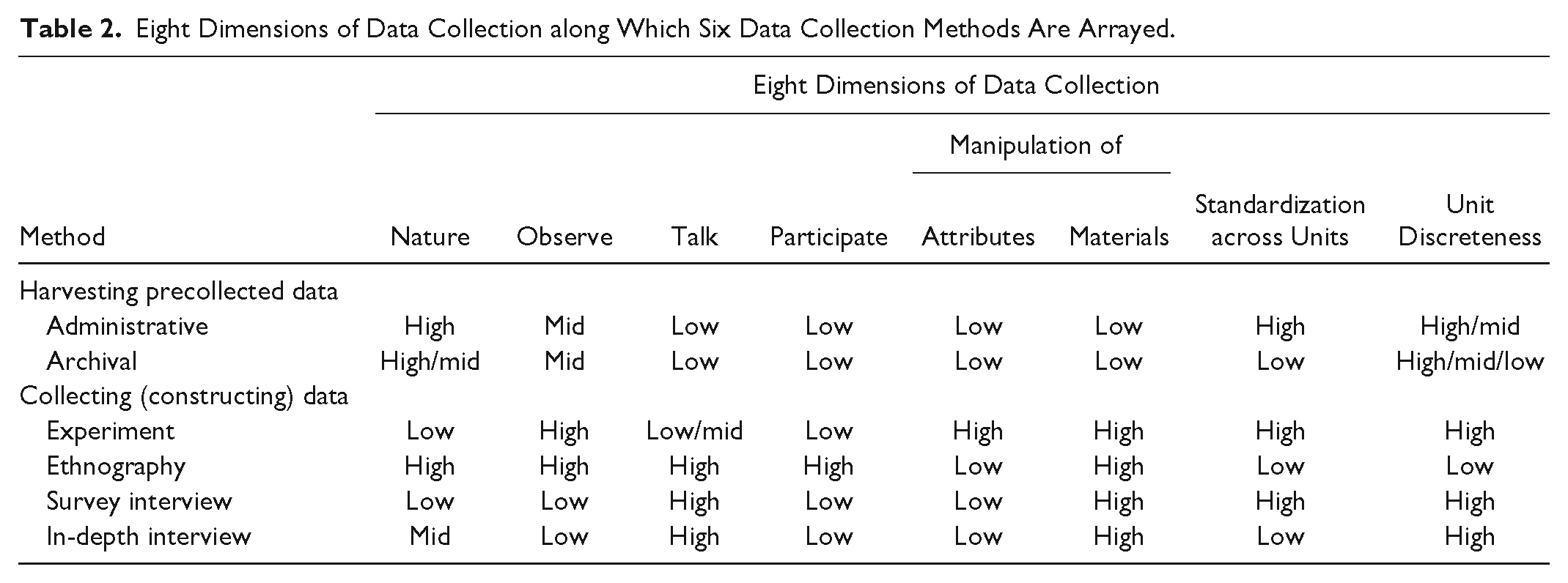
Table 2 shows that administrative and archival data match on every dimension except the degree to which information on units is standardized, possibly unit discreteness, and possibly the nature of the research site. Administrative data are standardized because administrators standardize record keeping even as reality is likely messier. 19 Archival data vary so much that archival researchers often cannot treat data in a cross-unit standardized manner.
Surveys and experiments differ only in the use of observation, talk, and their varied ability to manipulate subjects’ attributes.
Ethnography, however, is visibly unique. High on all dimensions of interaction—talk, observe, and participate—ethnography is the only method that entails full presence in subjects’ lives. Perhaps for this reason, ethnography is also the only method that necessarily accesses holistic, connected subjects, rather than rendering them discrete units of analysis. Again, the structure of ethnography suggests the possibility of truly distinct, yet deeply coherent, epistemological commitments, in a way that may involve distinctly different case selection.
Notably, although both ethnography and in-depth interviewing are qualitative methods, they appear quite different. Perhaps tellingly, they differ on the natural dimension. Meeting someone in a coffee shop or his or her home for a lengthy conversational interview, however illuminating, is less embedded in members’ natural world than is engaging subjects in open-ended accompaniment to parties, to court, or even to the same shared residence (e.g., Whyte [1943] 1981; Goffman 2014). The two methods also differ on the use of observation, the dimension of participation, and unit discreteness.
The methods match on the use of talk, the inability to manipulate subjects’ attributes, and the ability to manipulate study materials. With the exception of their joint lack of cross-unit standardization, however, all dimensions on which they match also match the placement of survey interviewing. Hence, ethnography and in-depth interviewing, ostensibly two qualitative methods, uniquely match on only one dimension: the lack of standardization across units.
Indeed, it appears that in-depth interviewing has much more in common with survey interviewing than with any other method, differing only in the degree to which data collection is natural and the degree to which interviews are standardized across units. Consequently, any differences in case selection strategies for survey and in-depth interviewing likely must be justified on the basis of these differences.
Given each method’s structure, the ubiquity of social world lumpiness, and the necessity of generalizing in the extrinsic interest case, what is the advised deployment of the probability principle across each method’s relevant research moments? The next section addresses this question.
Method-specific Implementation of the Probability Principle
Any analysis of disparate methods risks being so abstract that discussants talk past each other. Yet because strong and weak examples of each method are published, citing specific studies rarely clarifies, as sensitivities easily escalate. Still, concrete examples can be helpful. Therefore, I first offer for each method an illustrative, fabricated study relevant to child abuse. While identifying the usual use of probability and nonprobability approaches in each method across the research moments, I offer advice on probability sampling sensitized by each methods’ architecture.
Six Illustrative, Fabricated Studies
Table 3 relates six possible studies of child abuse using common designs. The issue of child abuse poses big questions. The challenge of nurturing children’s growth and autonomy, simultaneously protecting their bodily integrity, while preserving parental authority for direction and day-to-day decision making touches on deep, historic societal and political issues. What is the boundary between public and private? What is a feasible, respectful, cross-generation compact, and how can it be enforced and maintained? Given cultural diversity, what is the state definition of abuse? Such questions are not made easier by the contingent nature of childhood and its temporal variation (e.g., Boli-Bennett and Meyer 1978; Heywood 2001; Stearns 2006).
Six Illustrative Studies of Child Abuse.

Note. CPS = Child Protective Services.
Answering such questions could provide deeper comprehension and policy relevant insights. Doing so requires many different types of research. With the diverse illustrative studies in Table 3, I explore how probability methods may be deployed. Affirmative means establish the feasibility of probability sampling for diverse methods.
Probability Principles in Administrative Data Research
Administrative data capture entities conducting regular business, and thus entities are captured in highly natural contexts. 20 The data harvester cannot assign entities’ attributes (though administrators may). High standardization of discrete units also characterizes the method.
The combination of attributes does not justify nonprobability sampling designs. The Table 3 study treats the administrative data sample as the population, but the sample is nonprobability because some abused children are never evaluated for foster care placement. Analysts have long known that those who gain program administrator attention often do not match the full population of those who should gain administrator attention (e.g., Hampton and Newberger 1985). Both inappropriate inclusions and exclusions are patterned by social world lumpiness (e.g., Hampton and Newberger 1985), likely producing selection bias.
Table 4 arrays the three moments of research, darkening cells deemed irrelevant for administrative data. 21 It indicates that to avoid the problem, analysts should use administrative data whose intake process entails recording the status of the full population (or a probability-sampled section) of research interest. For example, in some jurisdictions, all children must either be vaccinated or explicitly request a vaccination waiver (e.g., Seipel and Calefati 2015). Were children’s abuse status assessed as their vaccination status or waiver request is secured, the resulting administrative data could cover the population, facilitating both child protection and analytic possibilities.
Moments and Submoments of Administrative Data Research: Common and Advised Designs.
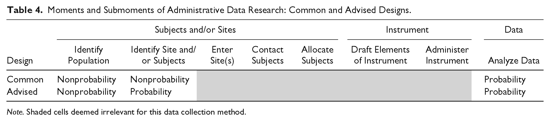
Note. Shaded cells deemed irrelevant for this data collection method.
Probability Principles in Archival Research
As Table 2 indicates, administrative and archival data collection differ trivially, and as there is no basis for nonprobability sampling in the former, there seems no basis for it in the latter either. Notably, archival analysts are aware that the preservation of primary (e.g., Earl et al. 2004) and selection of secondary (e.g., Lustick 1996) sources can eventuate in distortive selection bias. However, the highly nonstandardized nature of archival data, archival researchers’ need to immerse themselves in residues of the processes concerning their phenomena of interest, and their often holistic focus make probability sampling artifacts (e.g., diary pages) often inadvisable. The selection of specific artifacts is rarely the place for probability sampling.
Often archival researchers discover a particularly well-maintained set of materials and craft a question around those materials. In the Table 3 example, Michigan’s archives are posited to be especially extensive. If Michigan is selected to reveal how the phenomena work inside and outside of Michigan, then the problem is that the processes that lead the Michigan archive to be especially extensive may make Michigan a unique (i.e., ungeneralizable) case.
To address this problem, researchers should sample one or more jurisdictions for study (see Table 5). Indeed, analysts could even include in the study population states that neither passed nor considered such legislation, because relevant issues could arise in such states (e.g., at hearings on education, health, or child welfare generally). The analyst could stratify states by whether legislators voted on a child abuse law and/or knowledge of state archive quality, and states in some strata could be sampled with certainty. The advised approach is consistent with evidence that the “nonevent” is a staple of solid comparative research; for example, although Skocpol (1979) eschewed probability sampling, she selected nonevent cases in an effort to secure analytic leverage. The same logic can be applied in probability sampling to even better effect (Geddes 1990).
Moments and Submoments of Archival Data Research: Common and Advised Designs.

Note. Shaded cells deemed irrelevant for this data collection method.
Note that the point of probability sampling is not to estimate the “average” experience of U.S. states but instead to prevent an exceptional case from warping our understanding of how views of childhood, poverty, parental responsibility, and public-private relations in advocacy and legislative analysis are articulated and negotiated. There are only two ways to accomplish this aim: (1) study all cases, or (2) study one or more cases selected in a way independent of state idiosyncrasies. And the only way to do the latter is to probability-sample.
Probability Principles in Experiments
Despite “natural” experiments (e.g., Goldin and Rouse 2000), the common experiment occurs in contrived conditions. Experimenters primarily observe outcomes of discrete research subjects after manipulating both the characteristics of subjects (e.g., exposure to treatments) and the data collection materials, and the aim is to test whether a given intervention or condition is or can be causal. Experiments are not meant to estimate population characteristics or generalize to a population. If analysts truly avoid generalizing, there is no problem with current practice.
However, generalizing experiment-based findings is difficult to avoid. Experimenters and their readers often draw broader inferences. For example, analysts often reference Steele’s (1997) experiments on stereotype threat in an effort to explain group differences. Steele showed that stereotype threat can be causal but does not establish that effect in the population. Other work was needed to establish that fact (e.g., Huang 2009). Before such observational research, we did not know whether other factors were such that stereotype threat had no effect outside the lab.
The example suggests that it is difficult to avoid generalizing experiment-based findings. Although accepting the undeniable value of experiment-based evidence, the difficulty motivates interest in finding ways to conduct experiments that allow inference beyond the existence proof. To that end, we must first interrogate common practice to discern the factors that undermine generalizing from experiments.
Table 6 indicates that experimenters randomly assign persons to groups. Yet subjects are obtained via nonprobability processes. One common tactic is to allow undergraduates to satisfy course requirements by joining a subject pool. The Table 3 analogue is to use social work students to draw inferences about the process of removing children from their parents.
Moments and Submoments of Research Experiments: Common and Advised Designs.

Note. Shaded cells deemed irrelevant for this data collection method.
Researchers have criticized relying on college sophomores specifically (Sears 1986), but in response, some advise recruiting subjects from other, equally specific pools (e.g., shoppers; Henry 2008:65). The problem is actually twofold: (1) most pools are haphazard sets of entities, and (2) subjects are recruited rather than sampled from the pool.
As for pools, most do not represent a full population of real interest. Obvious differences between college sophomores and the wider public (e.g., less life experience, incomplete brain development [Johnson, Blum, and Giedd 2009]) underline this weakness, but differences of potential consequence distinguish other ostensibly general categories. For example, those who shop differ from those who do not (i.e., others shop for them). Indeed, most pools that appear universal actually are functionally haphazard collections, almost guaranteeing bias (see Henrich, Heine, and Norenzayan 2010 for an illuminating analysis).
The second problem arises because subjects are recruited from the pool. Recruits from any pool may be especially (non)susceptible to treatment. Thus, one cannot even justify generalizing from study participants to the unstudied members of the pool.
These claims are uncommon enough that an example may be helpful. Were an analyst to recruit subjects to study a preventive treatment for the common cold, those more susceptible to colds may be more likely to volunteer. If so, after randomly assigning subjects to treatment and control the results might easily show no effect of treatment; for example, if both groups are so susceptible to colds that even good treatments may fail, one will find no difference between volunteers who did and did not receive treatment. Yet the treatment might be very effective in the unstudied remainder of the pool or population. If one limited the conclusion to “the treatment has no effect in recruited subjects,” all is well. But as an indication of the treatment’s broad value, the recruitment of interested subjects biases study results and, in this case, mischaracterizes a possibly effective prophylactic. The problem can be much more subtle; for example, even if study aims are hidden during recruitment, volunteers and nonvolunteers for research may differ in relevant, unknown ways.
Thus, using a subject pool (instead of a population) undermines all inferences beyond the pool, and recruiting from rather than sampling of the pool undermines all inferences to the pool.
At least three responses follow directly. One response is to replicate each experiment on subjects from multiple dissimilar pools. The strategy constitutes a full employment program for experimenters, for one will never exhaust the groups possible for yet another experiment, and one still cannot generalize beyond the studied groups without asserting general linear reality (Abbott 1988). A second response is to use C2CT to draw inferences beyond the subject pool. The promise and risks of C2CT were noted earlier.
Alternatively, a three-step probability process could be used. In step 1, a population is identified. In step 2, a probability sample is selected from the population. In step 3, selected subjects are randomly allocated to treatments. The surest response to the generalization problem is the three-step solution.
Probability Principles in Ethnographic Research
That ethnographers collect data in natural settings on units embedded in real life suggests that ethnography is a truly distinct method. Presumably, an ethnographer could use a probability mechanism to decide whether to follow one person into the house or another down the street. However, applying probability methods in this way would threaten access to the very emergent reality ethnographers seek to reach, an emergent reality among contextualized units of interest. This bedrock reason against unreflectively, imitatively deploying probability methods on research subjects, flows from ethnography’s position on the eighth dimension of data collection, unit discreteness. Considering this dimension, however, reveals a surprise: some ethnographers arguably use probability methods!
Because this contention contradicts dominant views of ethnography, it is unlikely that a hypothetical illustrative study, as in Table 3, can clearly reveal the general feasibility of probability sampling. Consequently, I discuss published ethnographies in treating the issue.
Returning to the eighth dimension, we ask, What is the ethnographic unit of analysis? In describing residents’ flight from the police, Goffman (2014) provided a clue, writing, In my first eighteen months on 6th Street, I observed a young man running after he had been stopped on 41 [sic] different occasions. Of these, 9 involved men fleeing their houses during raids; 23 involved men running after being stopped while on foot (including running after the police had approached a group of people of whom the man was a part); 6 involved car chases; and 2 involved a combination of car and foot chases, where the chase began by car and continued with the man getting out and running. (p. 25)
Superficially, counting seems to be the analytic method, and the unit of analysis seems to be the event. But counting is not the analytic method, and a close read reveals the unit of analysis to be experience, not the event. Upon noting that 24 “runners” escaped, Goffman (2014) continued, Running wasn’t always the smartest thing to do when the cops came, but the urge to run was so ingrained that sometimes it was hard to stand still. When the police came for Reggie, they blocked off the alleyway on both ends simultaneously, [1] using at least five cars that I could count from [2] where I was standing, and then ran into Reggie’s mother’s house. Chuck, Anthony, and two other guys were outside, [3] trapped. . . . Anthony had the warrant for failure to appear. As the police [4] dragged Reggie out of his house, laid him on the ground, and searched him, [5] one guy whispered to Anthony to be calm and stay still. [6] Anthony kept quiet [7] as Reggie was cuffed and placed in the squad car, but then [8] he started whispering that he thought Reggie was looking at him funny, and might say something to the police. [9] Anthony started sweating and twitching his hands; the [10] two young men and I whispered again to him to chill. [11] One said, “Be easy. He’s not looking at you.” [12] We stood there, [13] and time dragged on. When the police started searching the ground for whatever Reggie may have tossed before getting into the squad car, [14] Anthony couldn’t seem to take it anymore. He started mumbling his concerns, and then [15] he took off up the alley. One of the officers went after him, causing the other young man standing next to him to [16] shake his head in frustrated disappointment. (pp. 27–28; italics and counts added)
In the next few paragraphs Goffman (2014) concluded the episode, but what is evident in the reporting, and highlighted in the numbered instances above, is that the fundamental unit of analysis is the experience—its texture, rhythm, and depth—not an event. Goffman’s analysis of contour and affect, of the extension in time and space, captures the experienced reality that may issue from a condition, a circumstance, an event, a witnessed occurrence, or something else.
As another example, consider Anderson’s (1976:87–91) narrative concerning Tiger’s mobility. After obtaining a job, Tiger was a recent transplant from the “winehead” to the “regular” group category. Thus, his status was often contingent, at times motivating visible notice of his job status and displays of camaraderie co-created by Tiger and others. Such displays might solidify his mobility. Anderson related one such occasion, writing that, One evening just before six, the time when Tiger had to get ready for work, T.J. said in the presence of other regulars: [1] Many of the regulars, who only a few weeks before would not even take up time with Tiger, let alone drink with him, [12]
Other examples—such as Whyte’s ([1943] 1981:130–37) discussion of police-community relations and the sole officer who cannot be bought, Willis’s (1977:19–22) relation of lunchtime drinking on the last day of school, and MacLeod’s ([1987] 1995) contrast of the brothers and the hallway hangers—deepen the understanding of experience as the fundamental unit of analysis. Whyte ([1943] 1981:20–24) offered perhaps the classic example in his report on the corner boys’ bowling tournament. 22 These examples suggest that the ethnographer selecting a site (e.g., 6th Street) for study resembles a survey researcher selecting a country for study, for both usually make those selections nonprobabilistically. Within the site, however, case selection occurs (i.e., units of analysis are obtained for study).
After experience is posited as the unit of analysis, four questions arise quite quickly. First, what are the unit’s boundaries? The question seems to presuppose a discrete entity, whereas the unit for ethnography is not discrete. Figure 2 traces the difference between the usual unit of analysis (see panel A), a discrete entity (that might be nested in other entities), and the ethnographic unit of analysis. First, in panel B, overlapping segments represent multiple simultaneously occurring experiences (e.g., experiencing the possibility of arrest and positive affect toward one’s friend), indicating that experiences, although perhaps analytically distinct, may not be viscerally separable. Second, the fuzzy or tapered start and/or end of some segments indicate that experiences sometimes lack clear boundaries. Third, two or more segments on the same level indicate that an experience can be discontinuous, seeming to end only to continue later in time. Apparently, the terrain as studied is much more complex than in most research. Surely, some traditions sometimes question the individual or organization as a discrete unit of analysis, but for research to proceed analysts usually ignore the issue, at best interpreting it to allow simultaneous treatment of flows and/or multiple kinds of units. In contrast, in ethnography, the issue cannot usefully be ignored: the fundamental unit of analysis is an experience, an indiscrete, potentially discontinuous, fuzzily bound unit.
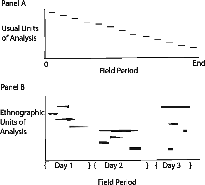
Usual units of analysis and ethnographic units of analysis collected over three days of the field period.
Second, if the unit of analysis is experience, how can one sample it? It is apparent that ethnographers sample the vessel in which experience is contained. Ethnographers sample time. This is apparent in Duneier’s (1999) observation of the “[Howard] Becker principle”: “most social processes have a structure that comes close to ensuring that a certain set of situations will arise over time” (p. 338). If “situations . . . arise over time,” then sampling time will bring the situations and the associated experiences into the analyst’s purview. We see this also in Anderson’s (1976) multiple reports of fieldwork in and around Jelly’s bar. In these cases and innumerable others, time is the vessel that contains experience.
Third, if the unit of analysis is “experience,” and time is its containing vessel, how may ethnographers be seen to use probability sampling? Basically, the de facto sample design of ethnographic research matches the experience sampling method (ESM) (e.g., Csikszentmihalyi and LeFevre 1989). In formal ESM designs persons are given pagers, cell phones, or cell phone apps that beep at random times. When beeped, the person is to record requested information about their activities, environments, and state of mind. ESM designs were used to establish the concept of flow and its relevance for optimal experience (Csikszentmihalyi 1990). The insight of ESM is that experience is embedded in time, and to access the emergent reality of experience while maintaining the integrity of experience, one must sample time.
Finally, one might wonder, to what can an analyst generalize who has sampled time to gather data on experience? One answer is that sampling time is akin to cluster sampling. In cluster sample designs, analysts sample higher level units in which lower level units are nested and draw inferences concerning lower level units (Kalton 1983:28–29). For example, one might sample two third grade classrooms in a school with five and draw inferences on the third graders in the entire school. Classrooms are just a convenient way to obtain students. Similarly, all experience is contained in time. Sampling time allows analysis of the experiences that occur in the sampled times and inference to experiences that occur outside the times sampled, just as sampling classrooms allows analysis of students in the cluster sampled classrooms and inference to students outside the classrooms sampled. In Goffman’s (2014) case, experiences emerged in the context of a hyperpoliced street, and the experiential data she obtained can be generalized to other experiences in that specific context. In a final inferential move, one may generalize beyond 6th Street via C2CT (i.e., to other hyperpoliced streets and/or other circumstances of stress and extremity), to the extent that one can show that the contexts match (because Goffman did not select 6th Street via probability sampling).
Ethnographers implement ESM by attending to their time in the field. Anderson (1976) reached Jelly’s bar at all hours of its operation and extended fieldwork beyond the establishment’s confines, while Whyte ([1943] 1981) moved to the neighborhood. When ethnographers randomly vary their fieldwork times within the range relevant for the site or immerse themselves in the site, their methods match ESM. 23 Surely, many analysts may reach the site at the same time each week and thus systematically miss some experiences (e.g., the texture of the street when children dash homeward from school). And even scholars who vary site visits may do so more around teaching days and committee work rather than via probability methods. 24 Thus, not every ethnography uses probability sampling. The “fix” for this is obvious: use a probability selection mechanism. Implementing this fix may require administrators to aid ethnographers’ flexibility in fulfilling campus responsibilities during data collection.
Table 7 summarizes the conclusion. Ethnography is sufficiently distinct to use a distinctive epistemology. Although delving into possible epistemologies for ethnography could illuminate other issues, it is unnecessary for case selection, for, despite its distinctiveness, probability sampling is feasible and indeed has been used when analysts relocate to the site. Even without relocating, the moments of field site entry may be decided via a probability process. This counts as probability sampling even though ethnographers may not view their fieldwork in such terms. But probability sampling by any other name is still as effective.
Moments and Submoments of Ethnographic Research: Common and Advised Designs.

Note. Shaded cells deemed irrelevant for this data collection method.
Probability Principles in Survey Interviewing
Table 8 reports the common and advised designs for survey interviewing. Survey researchers were spurred to probability sample after the infamous 1948 “Dewey Defeats Truman” headline, a headline that matched pollsters’ predictions on the basis of quota (i.e., nonprobability) samples (Frankel and Frankel 1987). Even so, the General Social Survey (GSS) used block quota sampling up until 1977 (Davis and Smith 1992), nearly 30 years after the Dewey election fiasco. More recently, survey interview data collection has extended probability principles to instrument design and implementation (e.g., Glynn 2013).
Moments and Submoments of Survey Research Interviewing: Common and Advised Designs.
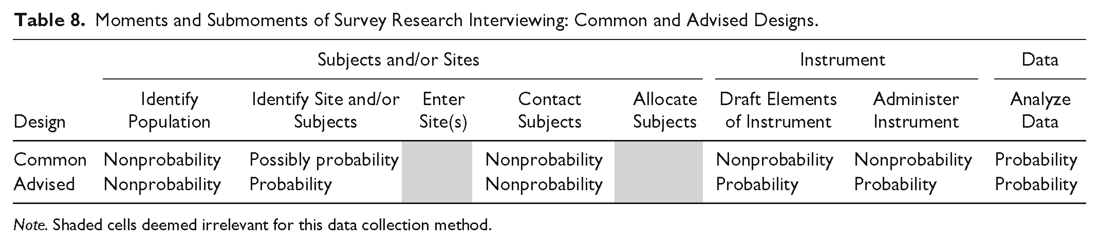
Note. Shaded cells deemed irrelevant for this data collection method.
Sample design issues sometimes receive insufficient attention when secondary data analysts use survey data, as in the Table 3 multilevel analysis of the GSS. Although geocodes are available, the GSS’s complex sample design prohibits using states (and most other geosocial levels) as units of analysis. Estimates from prohibited multilevel models have unknowable directions and magnitudes of bias (Lucas 2014b:1625–28). Generally, rarely can statistical models repair matters when one starts from a nonprobability design (Morgan and Liao 1985). Thus, researchers who respect data set limitations avoid estimating models the sample design prohibits. Alas, some analysts present such work without qualification.
Editors and reviewers cannot immerse themselves in every codebook, but research aims should not be undone by known data set limitations on the same date of publication. To ensure the latter, editors should require analysts to reference the specific codebook text showing that the sample design warrants estimation of each parameter of interest. This small change would eliminate literally dozens of misleading analyses, months of wasted reviewer time, and person-years of futile author effort each year, all while greatly increasing the likely veracity of our inferences.
Probability Principles in In-depth Interviewing
Heretofore the analysis indicates that in-depth interviewing is structurally dissimilar from ethnography, and some ethnographies use probability sampling. Thus, two main analogic defenses of nonprobability sampling for in-depth interviewing no longer apply.
The only two structural differences between survey and in-depth interviewing force a question: does interviewing in more natural environments and/or with low levels of standardization inherently require nonprobability case selection? Certainly, all interviews require the securing of cooperation, depend in part on rapport, and are interviewer and respondent co-creations (Suchman and Jordan 1990). Survey and in-depth interviewing seek validity differently given these conditions; survey interviewers standardize (Converse and Presser 1986) whereas in-depth interviewers individualize (e.g., Williams and Heikes 1993) the interview. The different strategies constitute differences on the nature and standardization dimensions, but as the findings on ethnography imply, these dimensions do not constrain case selection. Consequently, they cannot justify nonprobability sampling.
Of course, the Table 3 in-depth interviewer is required to engage an incredible set of skills: to inquire about stressful issues in nonthreatening ways; follow up with an uncanny combination of direction and empathy; and elicit sensitive information on persons’ experiences, understandings, and predicaments. The skills are impressive; equally impressive and expansive is that nothing about those skills limits their deployment to subjects selected nonprobabilistically. Yet for the Table 3 study, how could one probability-sample?
First, recognize that though few are formally charged with child abuse, clinically defined abusive acts are common (Hussey, Chang, and Kotch 2006). Thus, sampling an area’s population is a viable strategy. If one still fears that adults with the experiences sought for study will be rare, one could stratify adults as inside and outside the jurisdiction’s jail, justifying the stratification plan the same way one justified the original plan to study formerly incarcerated men. Stratifying by reason for incarceration is unnecessary because prosecutorial discretion and vagaries of jury decisions weaken the relation between jail, guilt, and charge. If authorities block access to incarcerated persons, one could still probability sample jailed persons as they are released (see Table 9).
Moments and Submoments of In-depth Interview Research: Common and Advised Designs.

Note. Shaded cells deemed irrelevant for this data collection method.
Once a restricted category (e.g., formerly incarcerated men) has been selected for study, it is easy to see how in-depth interviewers might struggle to imagine how to draw a probability sample. But a restricted category is rarely necessary, for usually the study focus (e.g., emotional and behavioral response in dealing with or abusing children) implicates others. Indeed, even if subject scarcity is a concern, complex sample designs, such as stratified or multistage sampling, can often address it. With such strategies, in-depth interviewers can draw the probability samples they need to solidify the basis for their unique inferential contributions.
Can Nonprobability Samples Be Salvaged?
Probability sampling can be difficult. Thus, it would be a wonderful breakthrough to find a means to use nonprobability samples. Alas, efforts to provide general, systematic means to repair such samples seem to either impose even more difficult to justify assumptions or to fail outright. Two examples illustrate the challenge.
Respondent-driven Sampling
Under respondent-driven sampling (RDS), respondents are recruited just as in snowball sampling. But at the end of the interview or survey, the respondent is given coupons to deliver to eligible contacts who might take part in the study. For every contact who proves eligible and participates in the study, the original respondent receives compensation. The secondary respondent then also receives coupons. As wave after wave of contacts become respondents, analysts monitor categories of respondents to determine whether they reach a stable composition and/or whether size requirements are met (Salganik and Heckathorn 2004).
RDS has been widely used in epidemiological studies of hidden populations (e.g., Ramirez-Valles et al. 2005). RDS does not typically produce generally unbiased samples, yet critics note that RDS has difficult-to-establish requirements even for unbiasedly representing subsets of study interest. For example, for the method to work, the theory presumes that coupons are distributed at random through the network but, as Heimer (2005) noted, it is difficult to certify this criterion has been met, because we lack accurate information on the network at issue. It should also be noted that the method usually requires much larger samples than are typical for some research designs (e.g., qualitative studies). Finally, even some earlier developers have now shown that RDS does not repair nonprobability samples (e.g., Goel and Salganik 2010).
The Bayesian Savior Approach
A different effort seeks to adjust nonprobability samples using Bayesian model fitting and assumptions. 25 For example, Wang et al. (2015) first divided 750,148 Xbox gaming platform 2012 election poll responses into 176,256 categorical cells on the basis of respondents’ sex, race, age, education, state of residence, party identity, political ideology, and 2008 vote choice. Using two multilevel models, the authors produced cell-specific proportions of vote for each candidate. To do so, they first predicted cell-specific propensity to select one of the two major candidates, and then, conditional on that propensity, the cell-specific probability of voting for Barack Obama was obtained. Both multilevel models include a term for the state-specific vote for Obama in 2008. Each model is estimated on moving “average” samples that contain a given day, d, and all three previous days.
These cell-specific estimates are then weighted by the distributions obtained from 101,638 respondents from 2008 election exit poll data. The claim is that this source disadvantages the analysis because it does not account for demographic change between 2008 and 2012 (Wang et al. 2015:984).
The example study has many unique features that undermine the method’s general utility. First, key to the adjustment is the reliance on prior election results in three places: (1) both cell-specific multilevel models use state-specific votes for Obama in 2008, and (2) 2008 exit polls provide information on the cross-cell distribution of the 2008 electorate. Use of this information raises two questions. First, given that the analysis simply adjusts Xbox data results toward previous results, why not just use the 2008 vote percentage for Obama as the estimate for all 45 days prior to the 2012 election, and dispense with the Xbox data altogether? In other words, if one simply drew a horizontal line at Obama’s vote share in the 2008 election, how off would one be?
Obama received 52.9 and 51.1 percent of the vote in 2008 and 2012, respectively. Considering Figure 3 of Wang et al. (2015) suggests that the horizontal estimator would do fairly well, often besting what I nonderisively term the Bayesian savior approach. Using Obama’s 2008 vote would have matched the Bayesian savior approach in correctly predicting Obama’s victory. Further evidence supporting the horizontal estimator is that 2008 and 2012 state-level support for Obama are correlated at .98. Using correct prediction as the criterion, there seems little reason to prefer the complex procedures invoked over the simple horizontal estimator.
The general question the use of 2008 data raises, however, is whether the 2012 election is too easy a test of the method. The question—will the Republican or Democrat win the election?—is in fact one of the easiest cases in the social sciences (as evidenced in several decades of polling and television networks’ almost always correct presidential election projections). The binary choice entails a severely limited decision space. Were that space to expand (e.g., 16 options with multiple selections possible and where order matters), the data demands would too. Would adjusting nonprobability samples be so successful under such circumstances that one would be willing to forego probability sampling with confidence that the Bayesian savior method would work?
Furthermore, using “previous vote” data given the extremely high cross-time correlation in the vote (by state and within person) makes it difficult for the method to fail, because one year’s data are almost completely the same as the next. Although this is laudable for election polling, many areas of study have much lower cross-observation correlations, making the use of such data less helpful.
In addition, U.S. elections have been run for more than 200 years, probability sample–based election polls are conducted hourly over several months in the run-up to the election, and election exit polls produce volumes of data the Bayesian savior approach used to tweak its weighting. Few areas of study are blessed with such a bounty of information on which to draw.
Finally, the method weighs respondents’ answers by patterns in the relation between sociodemographic and ideological positions and voting in previous elections. This strength becomes a weakness if other characteristics rise to greater importance in an election, or if relations were to greatly change (e.g., if blacks respond to Republican proposals on immigration by switching parties in the belief that closed-door policies will tighten labor markets). Generally, if historic patterns break, the method will be compromised.
Continuing to search for means to repair nonprobability samples is a worthwhile task. Who knows, a breakthrough might occur that will greatly ease all our efforts. However, it should also be noted that the idea that mashing, stretching, blurring, and smudging bad information can turn it into good information is powerfully seductive. To resist the spell, researchers’ default behavior should reflect a commitment to probability sampling because, at present, it is premature to certify Bayesian modeling and assumptions as the savior of nonprobability sampling.
Addressing the Many Possible Ways of Attempting Repair of Nonprobability Data
There are innumerable ways one might propose for repairing nonprobability samples. Some entail mimicking strategies used on probability-sampled data. For example, a common procedure is to accumulate and analyze multiple probability samples (e.g., Alwin and McCammon’s [1999] use of 22 GSS samples). Probability samples can be accumulated because knowing each case’s inclusion probability allows analysts to ensure that each case and thus each sample is properly weighted. Because nonprobability data lack inclusion probability information, proper weighting cannot be certified (Lucas 2014a:394–96). Thus, prior to any effort to combine samples, as in Hodson’s (2004) study of organizational ethnographies, one must ask whether (1) the samples involved are composed of probability sampled units and (2) the entities to be compared (e.g., schools, cohorts) are justifiably comparable. 26 Answering both queries in the affirmative affirms that the design is solid, but doing so means that one is not really repairing nonprobability-sampled data; one is using probability-sampled data in a new way.
Of course, the possible repair efforts are legion, making it impossible to address each one. But a general guide may be helpful: before attempting to repair nonprobability-sampled data, consider whether the repair depends on assumptions consistent with the epistemological grounds for collecting nonprobability-sampled data. If not, the repair is contradictory. Indeed, it is likely that a successful, noncontradictory repair is impossible.
Eight General Efforts to Justify Nonprobability Case Selection
Despite the necessity and feasibility of probability sampling, eight general moves are available to maintain nonprobability sampling. Assessing these moves, however, dashes all lingering hope for nonprobability sampling.
The Real Contribution of the Work Is Theoretical
One claim is that the real contribution of nonprobability sample studies is theoretical. The claim is odd because theories set the direction for empirical research. The claim implies that research likely to lead scholars astray provides acceptable points of departure for new theory-focused research.
This use of nonprobability sampling is unnecessary, however, because sociology embraces theory. Some journals publish theory exclusively, general journal editors seek to publish theory (e.g., Kalleberg 2012:2), and sociology’s figurative pantheon is well populated by theorists. Many analysts publish pure theory (e.g., Bourdieu 1986; Breen and Goldthorpe 1997; Wright 2006; Lucas 2008, 2009) that provides the foundation for empirical study using appropriate data (e.g., Carter 2005; Breen and Yaish 2006; Dixon, Fullerton, and Robertson 2013; Lucas 2013; Bernardi 2014). The uptake of pure theory in empirical research obliterates any reason to attach low-quality empirical analyses to solid theoretical work, especially as the flawed findings warp understanding, research priorities, and policy development unless and until corrected—or longer.
Disclose Characteristics of the Nonprobability Sample
Another response is to disclose the nonprobability sample’s characteristics (e.g., one third of respondents are retired, half are married). The response resembles the reporting of probability sample descriptive statistics. Because observables and unobservables from probability samples relate in known ways, reporting descriptive statistics allows analysts to bound inferences by estimating the likely size, directions, and impact of sample-population differences on findings.
Alas, observables and unobservables of nonprobability samples relate in unknown ways, dissolving the basis for using nonprobability sample distribution information to bound inference in any manner at all. Thus, reporting nonprobability sample distributions offers only ritualistic value.
Assume Homogeneity
If one assumes enough homogeneity to collapse each nonstudy factor to one value (i.e., to degenerate distributions), unobservables cannot warp nonprobability sample–based findings. The assumption stipulates that within-category variance equals zero, equating the needed sample size and the number of categories compared, perhaps to as few as two. 27
Most proponents of nonprobability sampling are reluctant to use such samples. But if homogeneity is high enough to justify nonprobability sampling, it is high enough to use one case per analytic cell. Evidence indicates that homogeneity is a poor assumption, so analysts are right to recoil from it. But if the assumption is poor, so is the method that requires it. Rejecting the homogeneity assumption while accepting nonprobability sampling is contradictory.
No Realized Sample Is a Probability Sample
Some sampled persons refuse to participate in part or all of the study. Hence, most probability samples have missing data on variables and fewer than 100 percent of the subjects sought and thus are not full probability samples. Thus, the argument goes, real probability samples are no better than nonprobability samples, so both designs are appropriate.
This defense of nonprobability sampling fails because a probability sampling design makes it possible to assess the potential impact of nonparticipation or missing data. Indeed, with a probability sampling design, nonparticipation or missing data problems can sometimes be fixed (Little and Rubin 2002). Because unobservables from probability sample designs behave in known ways, repair efforts consistent with the probability sample design are possible. However, unobservables from nonprobability sample designs behave in unknown ways, making even an assessment of damage depend on assumptions that contradict nonprobability sampling.
These claims are relevant beyond survey or experiment-based research. For example, if 50 percent of a town’s men are single, but 25 percent of the men in the in-depth interview sample are single, the interviewer could assess the impact of this disparity on their findings in at least two ways. First, the analyst could reweight the sample to account for the skewed data (i.e., weigh the views of single men more than those of married men) and reanalyze the data. One approach would be to add x – 1 copies of each single man’s transcript to the data (if single men are weighed over married men with a ratio of x:1—in the example, x = 3). The analyst reading such weighted transcripts will obtain a (weighted) understanding of the phenomena. For more complex analyses, the weighted data could be read into analysis software. Comparing the findings from weighted and unweighted analyses of interview transcripts can reveal whether results are robust and, if not, the set of plausible findings.
Second, if the analyst recorded the number of contacts it took for interviewees to agree to be interviewed, the analyst could assess whether findings differ by intensity of effort needed to secure cooperation. If there is no difference in findings, one may reason that because securing the missing cases would have required increasingly intense efforts, yet intensity of effort needed to secure an interview is unrelated to findings, then obtaining the missing cases would probably have had no effect on the findings. Notably, such investigations and reasoning are justifiable with probability designs but unjustifiable with nonprobability designs (Lucas 2014a:394–96).
Consequently, we should not let the perfect be the enemy of the good. Probability sample designs, even given nonparticipation and unit nonresponse, dominate nonprobability samples.
Analysts Seeking Necessary or Sufficient Causation Do Not Use Probability Sampling
Goertz and Mahoney (2012:182–83) contended that analysts investigating necessary or sufficient causation do not use probability sampling. If study cases are of intrinsic interest, probability sampling is arguably unnecessary, but only because probability sampling is generally unnecessary for study of intrinsically interesting cases, not because of a focus on necessary or sufficient causation. Indeed, it has been established that necessary and sufficient causation are functional form hypotheses (Lucas and Szatrowski 2014:35–36), akin to logarithmic, logistic, complementary log-log, or other functional-form hypotheses and assumptions. The finding is key because the functional form of a relation is sensitive to the joint distribution of the factors of interest and thus can be distorted by configurations of factors being over- or underrepresented. The finding means that if cases are of extrinsic interest, probability sampling is as necessary for studying necessary or sufficient causation as it is for studying any other functional form. 28
Qualitative and Quantitative Work Flows from Two Different Cultures
In positing that qualitative and quantitative research occupy different cultures, Goertz and Mahoney (2012) clarified several methodological differences, usefully showing that some research challenges can be addressed in different ways. However, their analysis is descriptive, not evaluative (Goertz and Mahoney 2012:3). Yet all research designs are not equal; sometimes researchers sabotage their aims by inadvertently using ineffective designs. To identify such a situation requires a prescriptive analysis.
Research is just one of many areas in which description is no substitute for prescription. If some people attempt to fly from one rim of the Grand Canyon to the other by simply leaping off the canyon cliff, a descriptive analysis could note that behavior and even describe the thinking behind it. But would describing the “leap off the cliff” method make it acceptable or effective? The method’s problem would remain, evident in the visible and costly failures crumpled below, its problem traceable to leapers’ ignoring a key feature of the physical world (i.e., gravity). To any aiming to fly across the canyon, a prescriptive analysis, which might advise the use of aerodynamic forces to counter gravity’s inexorable pull, is more helpful.
Although the failures of nonprobability sampling are usually less visible, they are surely costly, and for similarly structured reasons; nonprobability sampling extrinsically interesting cases ignores the undeniable ontological fact of social world lumpiness. One must counter the force of social world lumpiness with other forces, not ignore it. And the only known means for analysts to counter the force of social world lumpiness is to use the power of probability sampling. Thus, on case selection, the qualitative-quantitative divide is irrelevant.
Sample for Meaning: Interpretivism Redux
Those who see their unit of analysis as meaning might aim to sample for meaning. And as the population of meanings is undefinable (because of the indeterminacy of possible meanings), they might reject probability methods.
Two responses are required. First, if one cannot identify a population, there is no target to which findings generalize. Thus, population definition is required for all rigorous research for cases of extrinsic interest. Second, just as ethnographers sample experience by sampling its containing vessel, to sample meaning one must sample its containing vessel, living beings. The need to sample living beings re-presents the social world lumpiness problem. Thus, failure to probability sample will lead to poor understanding.
Cost
A seemingly unassailable defense of nonprobability sampling accepts the value of probability sampling but, lamenting the financial cost of probability sampling, opts for nonprobability sampling designs. There are at least two problems with this approach. First, it is rarely based on an actual calculation of the relative costs. Usually the cost of probability sampling is simply assumed to exceed the cost of nonprobability sampling.
That the decision is based on assumption is important, because it leads to the second problem, which is that it emphasizes the (presumed) direct cost to the researcher while neglecting all indirect costs. Yet a proper evaluation of cost would also include multiple indirect costs. Among the many possible indirect costs, three kinds are easily noteworthy.
One indirect cost is the opportunity cost to the researcher of conducting research using methods known to fail. After using such methods, the analyst really has learned nothing generalizable (despite how the analyst may treat the results). The time and effort lost in making zero advance in general knowledge imposes an opportunity cost in that the researcher could have used other procedures. Even if the probability sample study advanced knowledge only a small amount, perhaps because of compromises to make probability sampling work (e.g., fewer cases), a positive advance exceeds in value the zero advance (or, worse, the negative advance; see below) a nonprobability sample design entails.
Knowing that one does not know something is better than knowing something that is not true, a fact which causes another indirect cost of nonprobability sample designs. Upon completing the nonprobability sample study, the analyst may now believe that he or she knows something (e.g., a theory worth probing, a phenomenon worthy of study). However, the knowledge is seriously flawed (and thus can be deemed a negative advance). A proper consideration of cost would include downstream missteps (e.g., studying phenomenon X or theory Y because nonprobability sample studies found it important or revealing of the meaning or lives of group Z members when in actuality it is not) the analyst is more likely to make having built their research agenda from findings drawn from nonprobability sample-based studies.
The analyst is not the only actor on which costs of nonprobability sample designs are imposed. Costs are imposed on other researchers in at least two forms. First, the research community is deprived of the knowledge the nonprobability sample analyst could have produced had the nonprobability sample analyst used a probability sample design; thus, the community will be unable to ground future research in those unobtained findings. Second, peer review, if nothing else, may require researchers to address the nonprobability sample–based findings in their own research, entailing wasted pages, time, and attention. Even stating that the nonprobability sample-based findings are ungrounded can be damaging in the peer review process, for it (1) takes space when word counts can be a severe constraint and (2) risks alienating some peer reviewers, who may then raise impossible-to-satisfy demands to greatly delay or even derail publication.
A final indirect cost to mention is imposed on all of us. Societal costs emerge when policy makers or other key societal actors (e.g., teachers, real estate agents, police officers) learn of nonprobability sample–based findings, accept the findings, and focus their attention or acts in accord with those findings. A brief example may solidify this point.
Upon analyzing their nonprobability sample of “Capital High” students in Washington, D.C., Fordham and Ogbu (1986) concluded that black students fail to achieve out of fear that peers would accuse them of acting white for doing so. Later, probability sample–based quantitative (e.g., Ainsworth-Darnell and Downey 1998; Cook and Ludwig 1998) and qualitative (e.g., Carter 2005) works rebutted the claim. Intriguingly, Carter (2005) found that when black students referred to others in this manner, they did not reference academics, targeting peers they viewed as behaving condescendingly instead. Academic achievers who were not seen as snobs were not so labeled. Thus, application of the epithet signified a rejection of snobbery, not a rejection of achievement. 29
Alas, for some the correction has come too late, as partisans and politicians have integrated the acting-white thesis into their worldviews. For example, in his 2004 keynote address to the Democratic National Convention, Senate candidate Barack Obama said, “Children can’t achieve unless we raise their expectations and turn off the television sets and eradicate the slander that says a black youth with a book is acting white” (Obama 2004).
This erroneous thesis may have affected teachers’ and others’ behavior toward black students. Indeed, a senator or president (Obama 2014) lecturing students to not believe something most did not believe anyway, and recruiting others to struggle against what evidence indicates is for almost all students a phantom menace, is hardly a way to nurture student trust or improve student learning.
Most claims about design costs assume prohibitive direct costs of probability sampling yet neglect the indirect costs of nonprobability sampling. Once the latter are considered, it is difficult to sustain the notion that costs generally align to justify nonprobability over probability sample designs. Indeed, the illustrative example above provides a sad, cautionary tale of the damage nonprobability samples do both to efforts to construct theory, identify patterns, or otherwise understand the social world on one hand and to societal efforts to secure the public interest on the other.
Concluding Remarks
Prior to the development of probability sampling, many believed that censuses provided the only way to study social phenomena (Kruskal and Mosteller 1980; Desrosières 2004:210–35). The breakthrough of probability sampling allowed generalizing about social phenomena from study of only some entities. Yet despite the epic, hard-won development of probability sampling, a method that liberates analysts from having to collect data on all population entities, some contend that some social science research methods not only need not use probability sampling but, actually, that probability sampling harms such works. Nothing could be further from the truth.
Probability sampling provides a cogent response to the undeniable ontological fact of social world lumpiness, a phenomenon that threatens all sociological analyses. Study conclusions justify analysts’ neglect of probability sampling principles in population selection, the first research submoment, while requiring all analysts to use probability principles in case selection, unless specific entities are of intrinsic interest or one seeks only an existence proof. Hence, the conclusions delineate diverse case selection traditions via a straightforward set of principles; identify areas needing improvement in all methods; and, by resolving confusion about case selection, facilitate cross-method dialogue on existing, productive epistemological differences.
The conclusions were reached by simultaneously considering six methods, preempting claims of favoritism, especially as damaging nonprobability samples were evident across methods. Indeed, even secondary data analysts, far removed from data collection, were shown to need to attend far more closely to sample design than currently.
The study produced several other findings and resources. The eight-dimensional array and moments and submoments of research aided the comparative study of methods and are resources for future comparative methodological analyses. Taken together the findings reveal that whatever value the quantitative-qualitative divide may have, it cannot justify case selection plans. (See note 30 for selected implications of the conclusions for training.) 30
Case selection produces analysts’ sole site for analytic access to the social world; truly, it is where the rubber meets the road. Probability methods ensure contact with the full, relevant social world and thus break unobservables’ power to misdirect; nonprobability methods break contact with the full, relevant social world and thus ensure unobservables’ power to misdirect. Unfortunately, the latter also makes damage assessment impossible.
Alas, inertia—resistance—may sustain nonprobability sampling. In his analysis of fundamental problems with many statistical analyses, Manski (1995) observed, Empirical researchers usually enjoy learning of positive methodological findings. Particularly pleasing are results showing that conventional assumptions, when combined with available data, imply stronger conclusions than previously recognized. Negative findings are less welcome. Researchers are especially reluctant to learn that, given the available data, some conclusions of interest cannot be drawn unless strong assumptions are invoked. Be that as it may, both positive and negative findings are important to the advancement of science. (p. 3)
We encounter a similar dynamic here. Fortunately, unlike in some situations, in which problems exist but solutions do not, the solution here is clear and feasible: draw probability samples.
Turning a sociological lens to inertia may explain its likelihood and suggest responses. Sociology is an individual and a collective enterprise. Although the field will gain if nonprobability sampling ceases, individuals may fear publishing fewer works (because any constraint reduces volume) in a field increasingly turning to counting publications to measure productivity. When counting publications displaces reading them, published works count equally regardless of design. In that context, probability sampling may be too costly for, if editors still publish nonprobability-sample-based works, the self-disciplining scholar pays with a shorter curriculum vita compared with peers. Outpublished scholars often receive less grant funding, lower pay, or a pink slip despite making important scholarly contributions. Given such dynamics, for which no single scholar is responsible, inertia is likely despite the damage and missed opportunity each nonprobability sample study entails.
Under such conditions, only a collective response may succeed in breaking inertia’s hold. Hence, it may fall to gatekeepers—editors, reviewers, and personnel committees—to require all analysts to prove that the threats social world lumpiness poses are addressed. (See note 31 for accompanying job market adjustments and implications.) 31 If the social world is lumpy and challenges all methods, then it is appropriate to place the burden of proof on all social scientists seeking access to scarce resources—including grant funding, journal pages, publisher prestige, and lifetime employment—to prove that they have taken appropriate steps to address those challenges such that when questions do not involve intrinsic interest in the studied cases, their findings apply beyond those selected for study.
Addressing social world lumpiness without probability sampling, and proving one has done so, are rarely if ever possible. However, if such proof becomes required, I submit that it will not long be needed. For in that environment, it will also not be long before secondary data analysts confine model estimation to appropriate data, and the heretofore largely untapped probability sampling creativity of those who collect data (e.g., in-depth interviewers) eventuates in effective probability designs becoming the norm.
The use of quota sampling in the GSS in 1977 suggests it took nearly 30 years from the embarrassment of “Dewey Defeats Truman” for survey researchers to universally embrace probability sampling, and it has been 30 years since promulgation of the acting-white thesis based on nonprobability sample–based research. It would be advantageous to avoid further high-profile missteps traceable to an issue as basic as case selection. Alas, to those not directly harmed by the woeful understanding and damaging policies to which poor research easily gives force, the costs of nonprobability sampling are often invisible. Yet the costs are no less real. A transmethod consensus in favor of probability sampling is necessary to avoid such costs in the future, to dissolve an unnecessary impediment to cross-method dialogue, and to bring the powerful insights sociologists can excavate with each method that much closer both to being found, and to being true.
Footnotes
Acknowledgements
I thank the two anonymous reviewers, Santiago José Molina (co-organizer of the Methods and Epistemology of Social Science Workshop), Martin Eirmann, Thomas Krendl Gilbert, Véronique Irwin, and Alex Bernard for comments on an earlier draft and Jan Jacobs, Susan Schacht (posthumously), H. Sorayya Carr, and Aimée Dechter for many helpful conversations. All errors and omissions are the fault of the author.