
Abstract
We examine the relationship between intangible intensity and the accuracy of analyst forecasts. Using an international sample of 2,200 firms during 2000–2016, we show that analyst accuracy decreases significantly when intangible intensity grows. In exploring the determinants of this effect, we distinguish between firm risk and the risk associated with intangibles. Our results reveal the role of financial reporting quality, ownership structure, and institutional quality in moderating the relationship between intangible intensity and analyst accuracy. Analyst forecast accuracy acts as a channel through which the higher levels of information asymmetry associated with intangible intensity affect the cost of equity. Our results are robust to different intangible intensity measures; mandatory changes in financial reporting standards; the implementation of transparency rules in certain industry sectors; and financial crisis periods. We have devised alternative econometric tools that deal with potential sample selection bias and the dynamics of our empirical model.
Introduction
Research has demonstrated the relevance of analyst activity as a mechanism to reduce information asymmetry and monitor managers’ activity and incentives (Ellul & Panayides, 2018; Hong et al., 2000; Yu, 2008). Information asymmetry will, ceteris paribus, be greater in firms with high intangible intensity, given that intangible assets are, by definition, more complex, and that estimates of their fair values are rarely disclosed. Moreover, the recognition and accurate measurement of intangible assets are more vulnerable to subjectivity than are tangible investments. In the same vein, firms with higher levels of intangible assets on their balance sheets are more likely to have unreported intangibles (Beaver & Ryan, 2005). Quite reasonably, therefore, in recent years, accounting standards have undergone changes aimed at reducing information asymmetry and the inherent complexity of intangible investments. The procedures that firms are required to follow under the IAS 36 (Impairment of Assets, 2004) are intended to ensure that assets are carried at no more than their recoverable amount, and to define how the recoverable amount is determined. IAS 38 (Intangible Assets, 2004) governs the recognition criteria and measurement models as well as relevant disclosures on intangible assets. Finally, IFRS 3 (Business Combinations), introduced in 2009, obliges an acquirer to recognize all identifiable intangible assets of the acquiree other than goodwill.
Within this context and given that financial analysts are among the major users of financial statements, Barth et al. (2001) find wider analyst coverage in the case of firms characterized by higher levels of intangible intensity. J. He and Tian (2013), however, show that wider analyst coverage implies a higher percentage of ownership held by non-dedicated institutional investors, as a result of which firm innovation is cut back to meet analysts’ near-term earnings targets.
Related to this, previous research reports a negative association between intangible intensity and analyst forecast accuracy (F. Gu & Wang, 2005; Higgins, 2013; Matolcsy & Wyatt, 2006). It has been recognized that intangible intensity may act as a proxy for firm risk and that riskier firms are, by definition, more difficult to value. The higher asset volatility of this type of firm may hinder analyst activity. Hence, the relevance of the relationship between intangible assets and accuracy of analyst forecasts may depend on the degree of information risk associated with each specific intangible asset. In this context, Jones (2007) states that the strength of this association appears to depend both on country-specific accounting policies for this type of asset and firms’ disclosure policies. His results provide evidence of a link between analyst forecast accuracy and intangible-related disclosure, in the sense that intangible asset forecasts may determine future earnings and thus convey potentially useful information to investors and analysts. This finding highlights the fact that the intangible intensity–analyst accuracy relationship is not entirely direct but is, rather, potentially dependent upon the legal-institutional framework within which the firm operates. Similarly, growing attention is being paid to firm-level variables with a direct influence on the severity of information asymmetries. Specific examples include studies incorporating ownership structure and corporate governance issues (see Anderson et al., 2004; Boubakri & Ghouma, 2010; Elyasiani et al., 2010; Piot & Missonier-Piera, 2009) and accounting information quality (see Anderson et al., 2004; Armstrong et al., 2011) when analyzing relationships among a firm’s various stakeholders.
The objective of this study is to conduct a deep examination of the relationship between firms’ intangible intensity and the accuracy of analyst forecasts. Using an international sample of 2,200 industrial firms for the period 2000–2016, we investigate whether the level of information risk associated with intangible assets could explain the negative association between intangible intensity and analyst accuracy. We also examine how corporate ownership structure and accounting reporting quality—from the firm-level perspective—and institutional quality—from the country-level perspective—affect the relationship between firms’ intangible asset investments and analyst accuracy. As an implication of this information-based argument on which our basic analysis depends, it is worthwhile to examine whether and to what extent the above relationships may be transmitted into a firm’s cost of equity.
This article contributes to the literature on the relationship between intangible intensity and analyst forecast accuracy in various ways. First, our results reveal that analyst accuracy decreases significantly with various measures of intangible intensity. We show, however, that the strength of this relationship differs depending on the type of intangible asset. In particular, we tested the relationship between intangible assets and analyst accuracy drawing a distinction between the levels of risk associated with different types of intangible assets, such as brands and patents, computer and software development, and licenses. The different degrees of tangibility in each type of intangible asset stress the relevance of considering their individual risk levels and, thereby, the potential of mechanisms, such as accounting rules, to increase the level of transparency for each type of investment. In relation to this, we find that firms in industrial sectors subject to specific disclosure requirements are perceived as less risky and are associated with higher levels of analyst forecast accuracy.
The overall significant negative relationship found between intangible investments and analyst accuracy is robust to a large set of firm-level controls and variables for analyst characteristics, such as analyst coverage and dispersion in consensus forecasts. Our results are also robust to the various regulatory changes in financial reporting standards introduced during our sample period and to the global financial crisis. In terms of methodology, we have defined alternative model specifications and econometric tools to deal with potential problems arising from sample selection bias and the dynamics of our empirical model.
The above relationship is likewise robust to firm ownership structure characteristics, which might also affect the degree of information asymmetry between the various stakeholders. In particular, after addressing potential endogeneity between ownership structure and analyst activity, bank ownership emerges as a more effective mechanism for reducing information asymmetry in intangible-intensive firms. This suggests a complementary error-reducing effect on analysts, albeit not sufficient to cancel out the overall negative effect of intangible assets on analyst accuracy.
Third, our results show that the relationship between intangible intensity and analyst accuracy is shaped by country-specific institutional quality, as proxied by different variables widely used in previous literature: (1) the quality of investor rights protection; (2) the degree of creditor rights protection; and (3) the quality of disclosure and transparency practices. In particular, our results show that the relationship between intangible intensity and the accuracy of analyst forecasts is more pronounced in institutionally weaker countries, where there are fewer mechanisms to reduce the information asymmetry typically associated with intangible assets.
Fourth, considering the findings of Easley and O’Hara (2004) and W. P. He et al. (2013), among others, we explore a direct implication of the negative relationship between firms’ intangible intensity and analyst forecast accuracy. Previous research supports the argument that analysts’ forecast accuracy could act as an additional mechanism to reduce information asymmetry between corporate stakeholders and might help to explain variations in firms’ cost of equity. To address this potential implication in our empirical context, we run a mediation test (Hayes, 2009, 2013; Shrout, 2011) to check whether the association between intangible intensity and the cost of equity is due, at least in part, to the mediating role of the accuracy of analyst reports. We also focus on testing whether the residual component of the equation describing analyst forecast accuracy in terms of intangible intensity (i.e., the portion of analyst accuracy not explained by the level of intangible intensity) affects the cost of equity. This analysis enables us to evaluate the loss of accuracy due to firms’ intangibility.
Overall, while corroborating the already widely demonstrated negative relationship between intangible intensity and analyst accuracy, our results show that informational complexity surrounding intangible investments emerges as one of the reasons underlying their impact on analyst accuracy. Our findings also show that some of the most negative aspects of this relationship may be partially mitigated by specific firm characteristics and country-specific institutional factors. Finally, the empirical findings of this article enable us to draw direct implications in terms of the increased cost of equity for the firm.
Literature review
Information asymmetry, analyst accuracy, and intangible assets
Pricing efficiency is very closely related to the efficiency of mechanisms for reducing information risk, which, in turn, is linked to the complexity of a firm’s assets valuation and, thereby, to its intangible investment intensity, among other variables (Barth et al., 2001; Hall, 2002). In this type of firm, there is greater information asymmetry between managers and external investors and more inherent uncertainty about firm value than is found in other types. In the case of intangible assets, higher uncertainty about firms’ investment projects may be consistent with at least two potential causes. First, firms with balance sheets reflecting higher intangible intensity may be more likely to have other unreported intangible investments. In relation to this, Beaver and Ryan (2005) claim that the higher uncertainty of intangible assets might be explained from an accounting-conservatism perspective. In their research, conservatism is understood as “the on average understatement of the book value of net assets relative to their market value.” In our context, conservatism has more to do with inception of assets and liabilities yielding expected but unrecorded goodwill (unconditional conservatism). Second, there is also the possibility of higher subjectivity in the recognition and measurement of intangible rather than tangible assets. This is particularly relevant in the case of intangible investments characterized by high risk and potentially low transparency. Both lines of reasoning indicate the existence of a link between higher intangible intensity and higher uncertainty, suggesting the need to develop regulatory and accounting tools to increase the level of accuracy when these types of assets are recognized on the firm’s balance sheet.
In line with the above arguments, we find evidence in previous literature affecting various company–stakeholder relationships. Aboody and Lev (2000), for instance, report higher insider trading profits in intangible-intensive firms, suggesting exploitation of inside information on R&D activities. From an earnings-management perspective, the reluctance of managers to disclose private information may be due to proprietary cost concerns (Verrecchia, 2001) or to uncertainty about the capital market’s response to disclosures (Nagar, 1999). Despite their role as sophisticated agents who may contribute to reducing information risk, financial analysts are not oblivious to the additional complexity of forecasting earnings for firms with substantial intangible assets. In fact, the literature has provided empirical evidence supporting a negative relationship between firms’ intangible intensity and analyst forecast accuracy (F. Gu & Wang, 2005; Higgins, 2013; Matolcsy & Wyatt, 2006). Thus, there is a need to identify potential mechanisms with which to reduce the information complexity of intangible assets to strengthen the benefits of more accurate analyst reporting.
The role of ownership structure and the institutional environment
Ownership structure
Previous literature has reported on the potential role of internal governance mechanisms in reducing information asymmetries and agency costs among the main company stakeholders. In terms of internal governance mechanisms, the mix of investor types may play a key role in determining the extent of agency costs due to information asymmetries between insiders and investors. Institutional investors are more sophisticated and better informed than non-institutional investors. Classical papers, such as Shleifer and Vishny (1997), show that institutional shareholders play a key role in reducing firms’ debt costs by monitoring and controlling management. Boubakri and Ghouma (2010) show that bond ratings improve significantly as the percentage ownership held by banks increases, ultimately causing the bond spread to narrow.
The effect of intangible intensity on analyst accuracy could, therefore, vary with the presence of institutional investors on firms’ ownership structure. This argument is rooted precisely in the role played by institutional investors in reducing information asymmetries, which take on special relevance in relation to this type of asset. According to Baysinger et al. (1991), long-term R&D projects are positively valued by institutional owners, who also tend toward portfolio diversification, which enables them to spread the higher inherent risk associated with intangible investments more effectively than is possible for less sophisticated stockholders. Furthermore, given their share in the firms’ capital, they usually find it harder to move efficiently in and out of stock positions. Thus, it could be argued that they have incentives to influence the return on their investment and, therefore, to adjust the information content of a large amount of balance sheet intangibles. This line of reasoning suggests that the presence of institutional investors can modify the impact of intangible intensity on analyst accuracy.
Consistent with the above, the presence of institutional investors might be expected to play a significant role in moderating the relationship between intangible investments and the accuracy of analyst forecasts, although the strength of that role might, a priori, vary between different types of institutional investors. Although previous literature has documented the role of institutional investors in reducing information asymmetries among a firm’s various stakeholders, it has also been argued that banks, in particular, may make a positive contribution toward more efficient external monitoring of corporate governance practices, given their privileged access to inside information (Fama, 1985; Datta et al., 1999; Pang & Tian, 2015). The simultaneous role of financial institutions as shareholders and specialized creditors may contribute further to reducing information asymmetry among a firm’s stakeholders during both financing and investment decision-making processes. In fact, the banking literature has posited that banks’ access to soft information through close lending relationships enables them to influence the efficiency of corporate investment decision-making. Previous papers claim that the participation of banks in their ownership structure benefits firms by facilitating their access to external funding and promoting efficient investment (Bris et al., 2008; Kroszner & Strahan, 2001). Hence, it is reasonable to expect the impact of intangible intensity on analyst accuracy to be moderated by the proportion of banks in the firm’s ownership structure. 1
Institutional environment
The Law and Finance literature has reported that an effective legal and institutional system that has the instruments and tools required to ensure law enforcement helps to overcome market imperfections caused by conflicts of interest and information asymmetries and thus promote financial development and economic growth (La Porta et al., 1997, 1998). Within this context, Claessens and Laeven (2003) explored the role of a country’s property rights protection in influencing the allocation of investable resources. Their argument relies, in particular, on the fact that a firm operating in a market with weaker property rights would invest more in fixed assets than intangible assets, because it would find it harder to secure returns from the latter than the former, regardless of the functioning of other alternative (internal or external) governance mechanisms. It can be said, therefore, that efficient capital allocation is more difficult in institutionally underdeveloped environments, where informational problems and agency costs tend to be more severe.
According to this information-based related argument, the quality of the legal and institutional framework may help to explain why analyst forecast accuracy could differ from country to country and how the perception of firms’ intangible asset investment policies may vary with institutional quality owing to the different informational environment in each country. In a similar vein, Leuz et al. (2003) argued that institutional quality—proxied by property rights protection, disclosure measures, stock market development, and ownership structure—helps to limit managers’ ability to acquire private control benefits and thereby reduces information asymmetry. Another potential repercussion of institutional quality is that strongly protected creditor rights may encourage firms toward cash flow risk reduction and more transparent investment policies (Seifer & Gonenc, 2012). Indeed, the role of institutional quality in the case of firms with high intangible asset intensity could be relevant not only because of the valuation difficulties inherent in this type of asset but also because of the higher level of risks and potential bankruptcy costs associated with such investments (Avand et al., 2015).
As providers of earnings forecasts for firms with different risk levels, financial analysts cannot be oblivious to the influence of the institutional environment. Just as a country’s institutional quality affects the degree of information asymmetry, so can it help to reduce the negative impact of intangible intensity on the accuracy of analyst forecasts. Hence, the quality of investor and creditor rights protection and the strength of corporate disclosure and transparency practices can influence the degree of information asymmetries particularly affecting firms’ intangible assets and, in this way, affect analyst accuracy.
Empirical design
Sample and database
Our sample consists of listed non-financial firms in France, Germany, Spain, the United Kingdom (UK), and the United States (US) examined during the period 2000–2016. All variables are expressed in US dollars and the data used in the analysis are an unbalanced panel of firm-year observations. The sample excludes firms whose analyst following may be influenced by special factors: the finance industry (SIC codes 60–69) and regulated enterprises (SIC codes 40–49, and 91–97). All variables are winsorized at the 1st and 99th percentiles to mitigate the impact of outliers. The accounting variables used to construct the proxies for intangible intensity—some of which are firm-level controls and institutional ownership data—were procured from the OSIRIS database (Bureau Van Dijk). Analyst forecast data were drawn from the FACTSET 2 database. The firms included in the analysis are all those with available data from the above-mentioned sources. We initially selected the 6,059 firms with available financial analyst data in FACTSET (47,350 firm-year observations). However, given the need to match the information provided by FACTSET with the data collected from OSIRIS, we restricted our final number of available observations to 16,395 firm-year observations and a maximum of 2,200 firms, including 438 for France, 306 for Germany, 72 for Spain, 625 for the United Kingdom, and 759 for the United States.
Variables
Analyst accuracy, intangible intensity, ownership structure, and firm-level controls
Our dependent variable is constructed from analyst consensus (median) EPS forecasts and annual EPS data drawn, as already stated, from the FACTSET database. As in Mansi et al. (2011), analysts’ EPS forecast accuracy is defined as the negative absolute value of analysts’ EPS forecast errors. Following Hribar and McInnis (2012), analysts’ forecast errors are calculated as the difference between actual EPS for the fiscal year y and firm i, minus the consensus (median) forecast for fiscal year y and firm i, scaled by the absolute value of the EPS consensus forecast. 3 In further agreement with these authors, we assess the sensitivity of our findings to low EPS by removing firms with absolute values of forecasted EPS below $0.10. Values close to 0 indicate higher accuracy, while those further from 0 indicate deviation from the consensus. 4
The main independent variable is intended to capture relative intangible intensity. Following Barth et al. (2001) and Claessens and Laeven (2003), among others, our basic measure of intangible intensity is the intangible-to-total assets ratio (INTANG) for firm i, in industry j, and country k, in period t. 5 To check whether the results vary across different types of intangible assets, we also considered (1) the ratio of brands and patents to total assets (BRAND); (2) the ratio of computer and software development over total assets (COMPUTER); and (3) the ratio of licenses to total assets (LICENSES). 6
The relationship between high institutional and bank-held ownership and analyst accuracy was examined by proxying for the proportion of institutional (bank) investors with a dummy variable which takes the value 1 if the percentage of institutional (bank-held) ownership is above the 90th percentile for the measure of institutional (bank) ownership and 0, otherwise (INST and BANK).
Since we also had to control for additional firm-level characteristics potentially affecting the accuracy of analyst forecasts, all the estimates of our model include BIG4, a dummy variable that takes the value 1 if the firm is audited by one of the Big Four audit firms, and 0 otherwise. We define firm size (SIZE) as the natural logarithm of total assets at the end of the previous year. LOSSEBIT is a dummy variable that takes the value 1 for firms with negative earnings, and 0 otherwise. We also include the standard deviation of RoA (DESVROA) over the past 10 years. 7 Finally, the control variables NUMEST and SIGMA are included to capture the number and dispersion of forecasts used to compute forecast consensus, respectively.
Institutional quality
As proxies for institutional quality, we followed La Porta et al. (1997, 1998) and Leuz et al. (2003), among others, and used both the index of protection of property and creditor rights. The property rights protection index was constructed by the Heritage Foundation to represent a country’s implementation of legislation to protect private ownership rights. The creditor rights protection index is computed as the degree to which collateral and bankruptcy laws protect the rights of borrowers and lenders. According to the Law and Finance literature, the effective protection of property and creditor rights requires both explicit legal protection and law enforcement. We, therefore, interact the above indicators with a variable to capture the quality of each country’s law enforcement. Specifically, we use the rule of law measure provided by the World Bank in Kaufmann et al. (2009) to define the interaction terms PROPRULE and CREDRULE. Higher values of these variables indicate both better property and creditor rights protection and better law enforcement. Finally, following Leuz et al. (2003) to capture specific features of the institutional environment surrounding disclosure policies and not directly included in either the property or creditor rights indices, we include two variables to proxy for corporate disclosure and transparency policies: DISC_L and DISC_WB, both of which are computed at country level. The first was calculated by La Porta et al. (1998) and later used by various researchers, including Leuz et al. (2003). The second is the country-level disclosure policies index computed by the World Bank and reported in the Doing Business dataset. Based on these institutional variables, we define subsamples of observations on which we regress our basic model for testing the relationship between intangible intensity and analyst forecast accuracy. For all four measures of institutional quality, we construct dummy variables that take the value 1 if the country’s specific institutional quality index is above the median value—computed for the entire sample of countries—and 0 otherwise.
Table 1 shows the distribution of firms across countries and industries. The descriptive statistics and the correlation matrix of the main variables of interest are shown in Tables 2 and 3, respectively. Variables definitions and sources are presented in Appendix I (Table 13).
Distribution of firms and observations per country and industry.
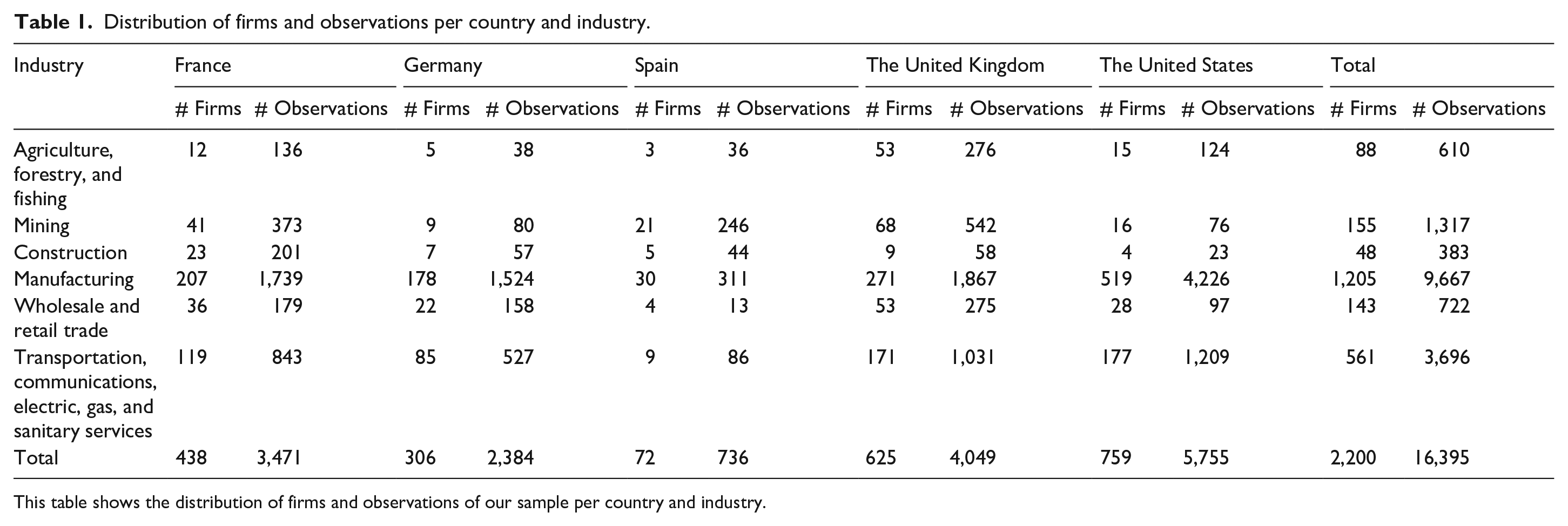
This table shows the distribution of firms and observations of our sample per country and industry.
Descriptive statistics.
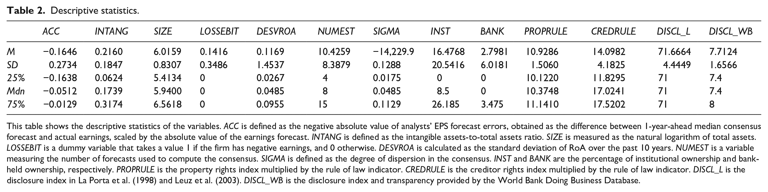
This table shows the descriptive statistics of the variables. ACC is defined as the negative absolute value of analysts’ EPS forecast errors, obtained as the difference between 1-year-ahead median consensus forecast and actual earnings, scaled by the absolute value of the earnings forecast. INTANG is defined as the intangible assets-to-total assets ratio. SIZE is measured as the natural logarithm of total assets. LOSSEBIT is a dummy variable that takes a value 1 if the firm has negative earnings, and 0 otherwise. DESVROA is calculated as the standard deviation of RoA over the past 10 years. NUMEST is a variable measuring the number of forecasts used to compute the consensus. SIGMA is defined as the degree of dispersion in the consensus. INST and BANK are the percentage of institutional ownership and bank-held ownership, respectively. PROPRULE is the property rights index multiplied by the rule of law indicator. CREDRULE is the creditor rights index multiplied by the rule of law indicator. DISCL_L is the disclosure index in La Porta et al. (1998) and Leuz et al. (2003). DISCL_WB is the disclosure index and transparency provided by the World Bank Doing Business Database.
Correlation matrix.
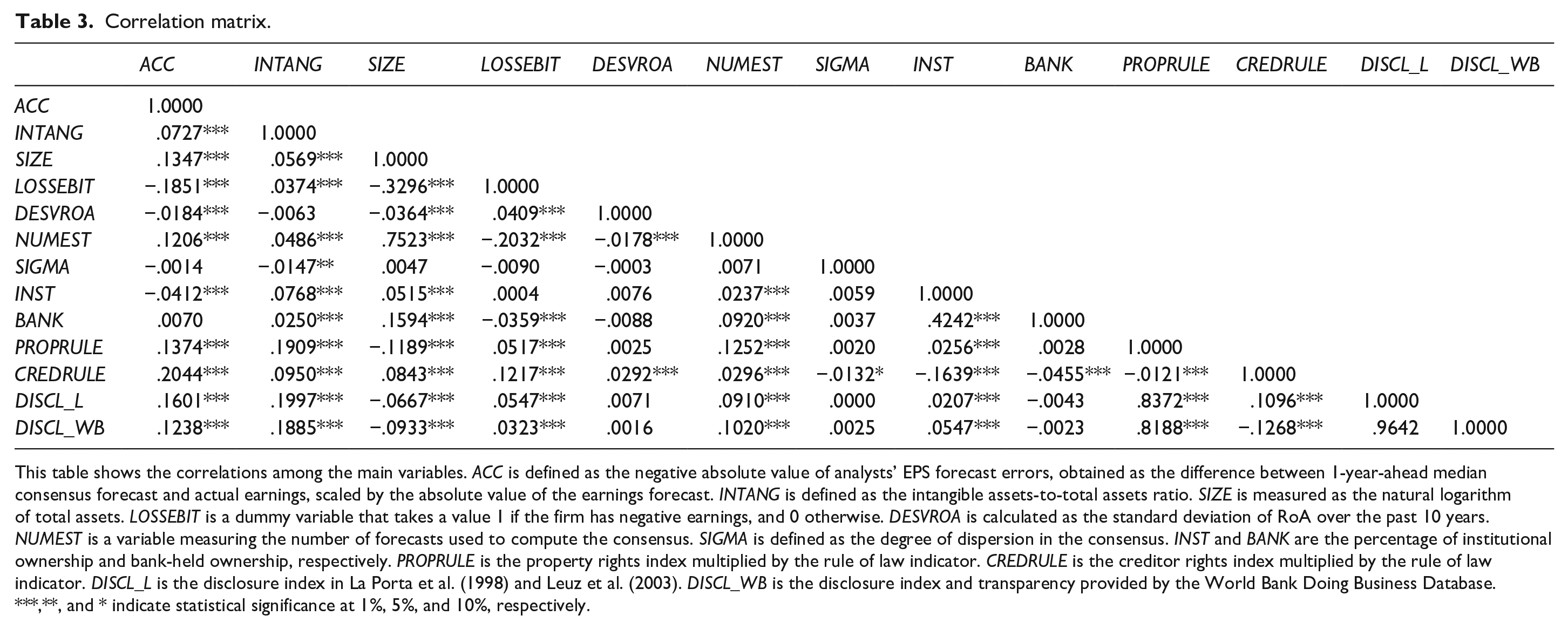
This table shows the correlations among the main variables. ACC is defined as the negative absolute value of analysts’ EPS forecast errors, obtained as the difference between 1-year-ahead median consensus forecast and actual earnings, scaled by the absolute value of the earnings forecast. INTANG is defined as the intangible assets-to-total assets ratio. SIZE is measured as the natural logarithm of total assets. LOSSEBIT is a dummy variable that takes a value 1 if the firm has negative earnings, and 0 otherwise. DESVROA is calculated as the standard deviation of RoA over the past 10 years. NUMEST is a variable measuring the number of forecasts used to compute the consensus. SIGMA is defined as the degree of dispersion in the consensus. INST and BANK are the percentage of institutional ownership and bank-held ownership, respectively. PROPRULE is the property rights index multiplied by the rule of law indicator. CREDRULE is the creditor rights index multiplied by the rule of law indicator. DISCL_L is the disclosure index in La Porta et al. (1998) and Leuz et al. (2003). DISCL_WB is the disclosure index and transparency provided by the World Bank Doing Business Database.
**, and * indicate statistical significance at 1%, 5%, and 10%, respectively.
Model specification
The basic model used to explore the relationship between analyst accuracy and firms’ intangible intensity is defined as follows:
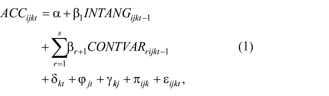
where the dependent variable is analyst accuracy for firm i, in industry j, and country k, at period t. All estimations include control variables
Our empirical strategy is likely to be affected by potential endogeneity concerns. Firms’ willingness to invest in intangible assets is likely to be endogenously determined and reverse causality is arguably possible. Although firms’ intangible intensity might logically be thought to influence the accuracy of analyst information, analyst activity (in terms of accuracy and recommendations) could also be justifiably argued to have some impact on firms’ investment policy. Hence, to avoid this potential econometric issue, in all our estimates, all firm-level control variables are lagged by 1 year to avoid simultaneity with the analyst forecast accuracy variable. 8
Finally, the basic estimation includes various alternative combinations of country-year
Our basic results are obtained using an industry-year cluster to capture correlations between different firms affected over time in the same country. We, therefore, apply the more general framework used in Petersen (2009), which avoids the need for assumptions regarding the specific form of dependence between the standard errors by employing a simultaneous two-level (industry and year) clustering approach.
9
Panel data analysis with random effects is used to account for unobservable firm-specific effects.
Empirical results
Intangible intensity and analyst accuracy
We begin by testing the impact of firms’ intangible intensity on the accuracy of analysts’ earnings forecasts. Columns 1 to 3 in Table 4 show different specifications of our basic model. In particular, Column 1 provides the estimates including country-year and country-industry fixed effects, and standard errors clustered at industry-year level. In Column 2, we show the basic estimates using country-year, industry-year, and country-industry fixed effects. The results of the estimates using only country-year fixed effects are shown in Column 3. As can be seen, this set of basic estimates provides empirical confirmation of a negative relationship between firms’ intangible investments and analyst accuracy. This is consistent with the basic argument found in the related literature associating higher intangible intensity with higher information asymmetry among company stakeholders, which causes analysts’ forecast accuracy to decrease. 10 This negative effect of intangible intensity on analyst accuracy also has economic significance. Based on the results in Column 1 of Table 4, for instance, an increase of one standard deviation in INTANG (0.1847) would result in a 2.9% decrease in the accuracy of analyst forecasts.
Intangible intensity and analyst accuracy.
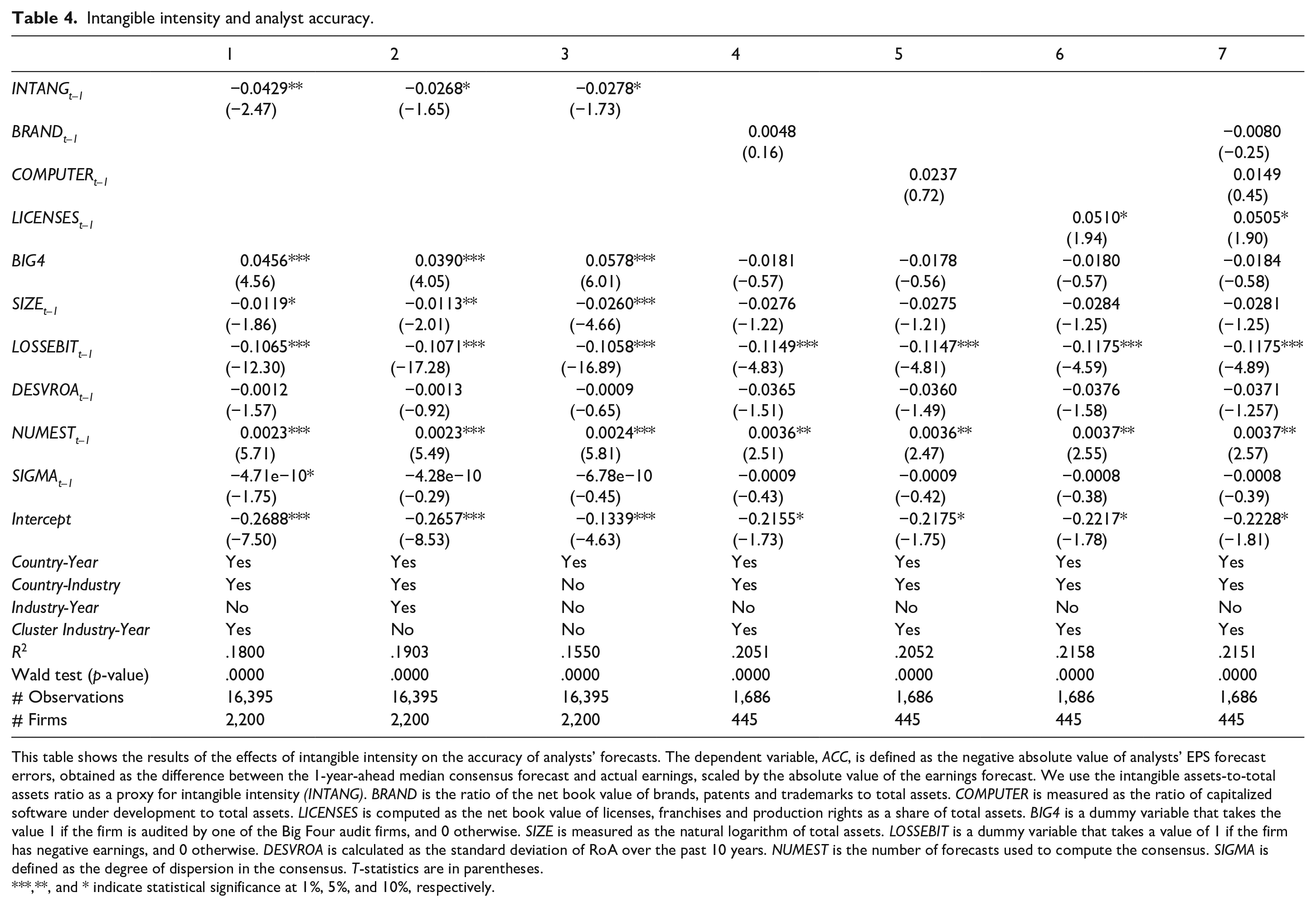
This table shows the results of the effects of intangible intensity on the accuracy of analysts’ forecasts. The dependent variable, ACC, is defined as the negative absolute value of analysts’ EPS forecast errors, obtained as the difference between the 1-year-ahead median consensus forecast and actual earnings, scaled by the absolute value of the earnings forecast. We use the intangible assets-to-total assets ratio as a proxy for intangible intensity (INTANG). BRAND is the ratio of the net book value of brands, patents and trademarks to total assets. COMPUTER is measured as the ratio of capitalized software under development to total assets. LICENSES is computed as the net book value of licenses, franchises and production rights as a share of total assets. BIG4 is a dummy variable that takes the value 1 if the firm is audited by one of the Big Four audit firms, and 0 otherwise. SIZE is measured as the natural logarithm of total assets. LOSSEBIT is a dummy variable that takes a value of 1 if the firm has negative earnings, and 0 otherwise. DESVROA is calculated as the standard deviation of RoA over the past 10 years. NUMEST is the number of forecasts used to compute the consensus. SIGMA is defined as the degree of dispersion in the consensus. T-statistics are in parentheses.
**, and * indicate statistical significance at 1%, 5%, and 10%, respectively.
In Columns 4 to 7, we replicate the basic model specification reported in Column 1 to examine the impact of different types of intangible assets on accuracy levels. The specific types of intangibles considered are as follows: (1) the ratio of brands and patents to total assets (BRANDS); (2) the ratio of computer and software development over total assets (COMPUTER); and (3) the ratio of licenses to total assets (LICENSES). We find a positive and statistically significant coefficient for LICENSES, shown in Columns 6 and 7, and no statistically significant coefficients for BRANDS or COMPUTER. The potentially higher tangibility and lower level of information risk associated with licenses (compared with the other two types of intangibles which, given their early stage of development, may be perceived as more opaque and/or risky), may enable financial analysts to achieve greater forecast accuracy. However, the size of our sample prevents us from drawing any strong conclusions from this specific set of empirical findings. 11
The remaining firm-level control variables show the expected sign overall. In Columns 1 to 3, BIG4 has a positive effect on analyst accuracy, thereby highlighting the positive role of financial reporting quality in reducing information asymmetry and thus increasing analyst accuracy. Firm size (SIZE) has a statistically significant negative impact on analyst accuracy in the first three columns. LOSSEBIT also has a statistically significant negative effect, whereby a negative income statement reduces analyst accuracy. A negative, albeit non-significant, impact on analyst accuracy is also observed for DESVROA. NUMEST, however, has a statistically significant positive coefficient suggesting that the greater the number of analysts following a firm, the higher the accuracy of their forecasts. SIGMA shows a negative coefficient indicating that lower consensus among financial analysts reduces their forecast accuracy. However, this result is statistically significant only in Column 1.
One important concern associated with our approach is the need to explain and demonstrate that the mechanism underlying our basic results is information-based. As previously stated, intangible intensity could be seen as a direct proxy for firm risk. Riskier firms (i.e., those with higher intangible intensity) are, by definition, harder to value and this volatility may hinder analysts’ ability to provide accurate estimates. However, given that investors are able to price risk, it is necessary to demonstrate that firms with comparable risk levels, but different amounts of balance sheet intangibles, differ with respect to the accuracy of their analyst forecasts. Thus, we could use our basic finding as an empirical grounding for our information-based theory and the study of whether and to what extent there are mechanisms (i.e., accounting standards rules, ownership structure, and institutional quality) that may contribute to alleviate information asymmetries would constitute a natural extension of this research.
In Table 5, we run our baseline regression across different subsamples of firms defined according to their level of risk, proxied by firm’s stock volatility, and their level of intangibility. In Panel A, we present the results when the value of the 25th percentile of risk and intangibility is used as the benchmark for our subsamples. Panels B and C report the results obtained when using the 50th and 75th percentiles, respectively. As can be seen, in all three panels, we obtain a negative and statistically significant coefficient for the variable INTANG in the subsample of firms characterized by higher risk and lower intangibility. This suggests that firms with high levels of risk (taking higher stock market volatility to be a priced risk factor) and less investment in intangible assets are those where the accuracy of analyst forecasts is least impaired as intangibility increases. In other words, among firms starting with comparable levels of stock return volatility, it is precisely those that are lower in intangible intensity that suffer most from the additional risk attached to this type of investment. This underscores the relevance of this additional source of risk, which materializes, as shown in Table 4, in lower analyst accuracy. The coefficient of INTANG in the case of firms with higher levels of both risk and intangible intensity is negative, although not significant at conventional levels. This would suggest that firms with larger amounts of balance sheet intangibles have, in fact, managed to capitalize on their intangible investments and investment strategy such that the associated risks have been already priced in. Hence, there is no room for increases in intangible assets to cause a significant reduction in analyst accuracy.
Intangible intensity and analyst accuracy across subsamples of firms with different levels of riskiness and intangibility.
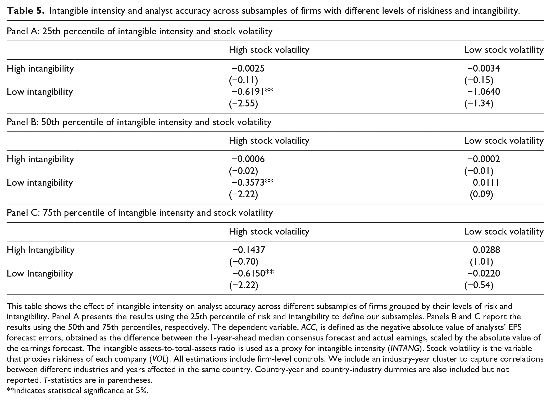
This table shows the effect of intangible intensity on analyst accuracy across different subsamples of firms grouped by their levels of risk and intangibility. Panel A presents the results using the 25th percentile of risk and intangibility to define our subsamples. Panels B and C report the results using the 50th and 75th percentiles, respectively. The dependent variable, ACC, is defined as the negative absolute value of analysts’ EPS forecast errors, obtained as the difference between the 1-year-ahead median consensus forecast and actual earnings, scaled by the absolute value of the earnings forecast. The intangible assets-to-total-assets ratio is used as a proxy for intangible intensity (INTANG). Stock volatility is the variable that proxies riskiness of each company (VOL). All estimations include firm-level controls. We include an industry-year cluster to capture correlations between different industries and years affected in the same country. Country-year and country-industry dummies are also included but not reported. T-statistics are in parentheses.
indicates statistical significance at 5%.
Intangible intensity and analyst accuracy: ownership structure and financial reporting quality
Having confirmed that larger amounts of balance sheet intangibles have a negative impact on analyst accuracy and that the mechanism underlying our basic results is information-based, the next issue for investigation is whether and how internal corporate governance mechanisms may affect the degree of the above-referred information-based mechanisms and, thereby, influence the basic relationship between intangible intensity and analyst accuracy.
The specific econometric model can be expressed as follows:
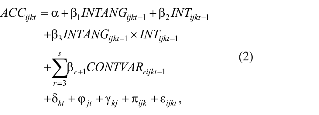
where the dependent variable is ACC; INTANG is used to proxy for intangible intensity; and INT is a vector composed of the variables that proxy for the role of institutional and bank investors in the ownership structure of each firm, namely, INST and BANK, and the measure of financial reporting quality (BIG4). The results are shown in Table 6. Column 1 describes the potential moderating role of BIG4; Column 2 shows the estimates obtained using the share of institutional investors (of all types) in the firm ownership structure (INST); Column 3 those obtained using the share of bank ownership (BANK); and Columns 4 and 5 present the estimates for different combinations of these variables to control for their moderating impact on the accuracy of analyst forecasts. According to the results shown in Table 4, the overall negative impact of intangible intensity on analyst forecast accuracy persists after controlling for the effects of financial reporting quality and ownership structure. Positive and significant coefficients are obtained for the interaction terms between our intangible intensity measure and the BIG4 dummy, and for the interaction term between INTANG and the proxy for the presence of banks in the firm ownership structure (BANK). This evidence is consistent with the claim that the negative impact of intangible intensity on analyst accuracy decreases significantly with financial reporting quality and in the presence of banks as shareholders; two factors with the potential to alleviate the information asymmetry associated with intangible assets. The interaction term INTANG × INST, although positive, is not statistically significant at conventional levels. 12
Intangible intensity and analyst accuracy: ownership structure and accounting quality.
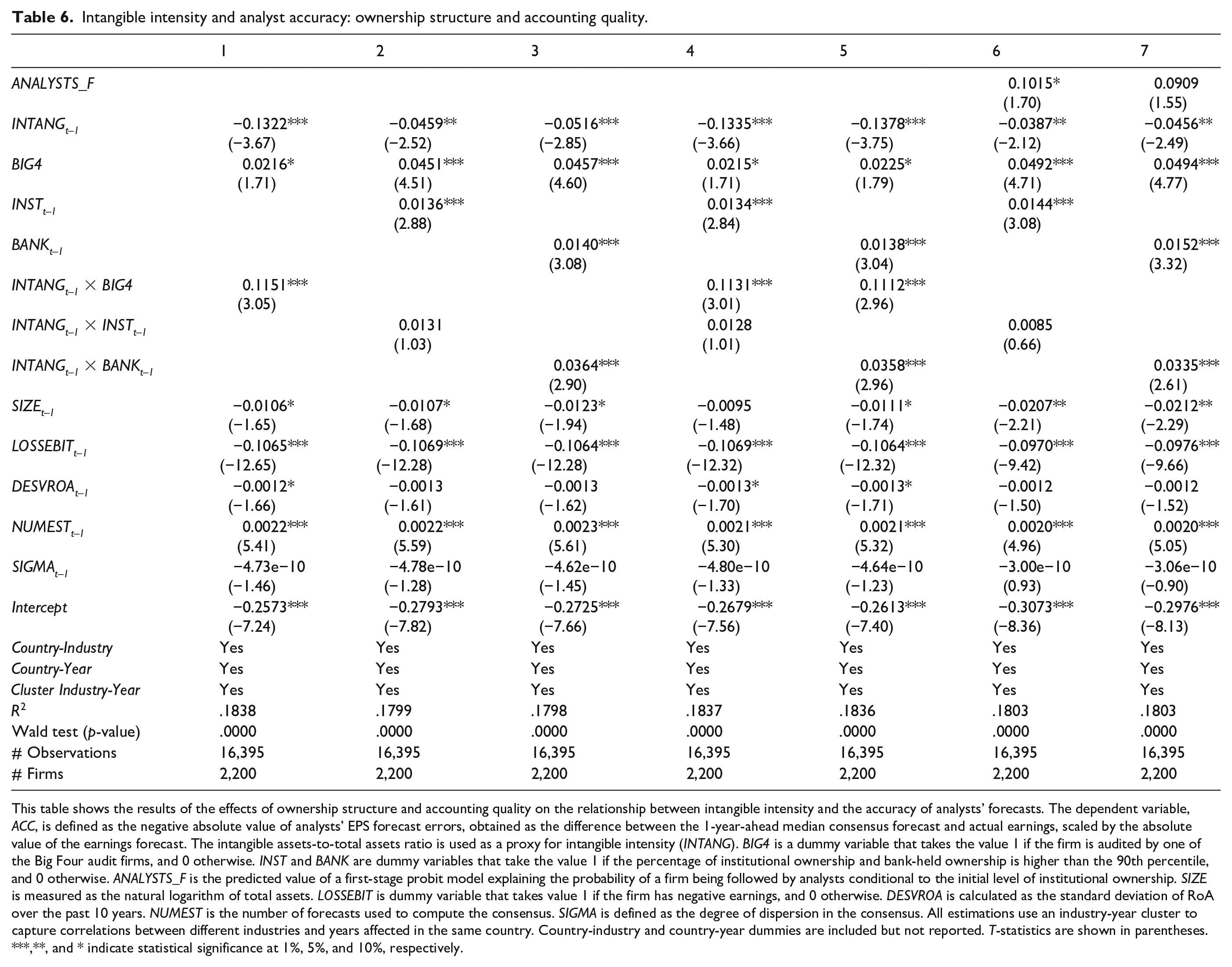
This table shows the results of the effects of ownership structure and accounting quality on the relationship between intangible intensity and the accuracy of analysts’ forecasts. The dependent variable, ACC, is defined as the negative absolute value of analysts’ EPS forecast errors, obtained as the difference between the 1-year-ahead median consensus forecast and actual earnings, scaled by the absolute value of the earnings forecast. The intangible assets-to-total assets ratio is used as a proxy for intangible intensity (INTANG). BIG4 is a dummy variable that takes the value 1 if the firm is audited by one of the Big Four audit firms, and 0 otherwise. INST and BANK are dummy variables that take the value 1 if the percentage of institutional ownership and bank-held ownership is higher than the 90th percentile, and 0 otherwise. ANALYSTS_F is the predicted value of a first-stage probit model explaining the probability of a firm being followed by analysts conditional to the initial level of institutional ownership. SIZE is measured as the natural logarithm of total assets. LOSSEBIT is dummy variable that takes value 1 if the firm has negative earnings, and 0 otherwise. DESVROA is calculated as the standard deviation of RoA over the past 10 years. NUMEST is the number of forecasts used to compute the consensus. SIGMA is defined as the degree of dispersion in the consensus. All estimations use an industry-year cluster to capture correlations between different industries and years affected in the same country. Country-industry and country-year dummies are included but not reported. T-statistics are shown in parentheses.
**, and * indicate statistical significance at 1%, 5%, and 10%, respectively.
Special attention is due to the moderating effect of bank ownership. As previously stated, reduction in the negative effect of intangible intensity on analyst accuracy in firms with a large bank presence in their ownership structure might be due to the dual role of banks as both shareholders and creditors of the firm. According to Hall (2002), intangible assets are more often financed with equity than with debt. The first reason for this has to do with adverse selection problems in the debt market, which are likely to be more severe for intangible investments. As previously argued, there is typically much greater uncertainty about returns to intangible than to tangible assets. Firms are also probably more aware than their lenders of the potential risks involved in such investments. In addition, debt financing can lead to moral hazard, given that intangible assets are more likely to encourage risk-shifting. In both cases, lenders may decide to cut credit or increase covenants in an attempt to control firms’ behavior (Jensen & Meckling, 1976; Stiglitz & Weiss, 1981). Third, intangible assets are also characterized by their low liquidation value, which would increase the cost of potential bankruptcy (Berger & Udell, 1990; Boot et al., 1991).
The dual role of banks as creditors with a significant percentage of shares in a non-financial firm may have an advantage over other types of institutional investors through privileged access to soft information about the firm’s investment and financial decisions. Traditional banking literature has confirmed the key role of financial entities in facilitating access to external funding for firms and ensuring efficient corporate investment through the establishment of close lending relationships with the debtor company (Petersen & Rajan, 1994, 1995). This is, in fact, the result of lower information asymmetry between the firm and the bank and could help to reduce the level of uncertainty traditionally associated with intangible investment strategies. Thus, from an outsider’s perspective, when it comes to issuing earnings forecasts and recommendations about the firm’s stocks, financial analysts stand to benefit substantially from reduced uncertainty enabling more accurate valuation of such firms and investments. This moderating role of bank ownership in the relationship between intangible intensity and analyst accuracy of analyst forecasts also has economic significance. Based on the results reported in Column 3 of Table 6, an increase of one standard deviation in INTANG (0.1847) of firms where banks have a strong ownership presence would mean a 2.45% increase in analyst accuracy.
At this point, it is necessary to acknowledge the potential endogeneity of the information environment, particularly as it might affect the role of financial analysts and institutional owners as internal corporate governance mechanisms with the potential to reduce information asymmetry. In this respect, it can be argued that institutional and bank investors may be inclined to demand more stocks from a firm that is being followed by analysts who are providing useful information (and even optimistic forecasts) about its future earnings. At the same time, analysts may start following, and even issuing optimistic earnings forecasts, for a firm if they see institutional demand for its stocks. The first of these issues can be addressed by including in all cases the lagged value of the proxy for the share of institutional investors in the firm ownership structure (INST and BANK). To deal with the second issue, we use a 2SLS method, where the first stage is to estimate the probability of an analyst to start following a firm. For this, we specify a probit model in which the dependent variable is a dummy which takes the value 1 if there is analyst information for the firm in a particular year, and 0 otherwise. In the second stage, we used the first-stage estimated probability as an additional explanatory variable to model the influence of institutional ownership on the accuracy of analyst forecasts. The results of the second stage are presented in Columns 6 and 7 of Table 6. ANALYSTS_F is the first-stage probability of analyst coverage, conditional to the baseline level of institutional ownership. 13 In line with previous findings, we document a negative effect of intangible intensity on analyst forecast accuracy. The results shown in Columns 3 and 5 still hold after controlling for potential endogeneity between analyst coverage and institutional ownership. We find a positive and statistically significant coefficient for the variable INTANG × BANK consistent with a weaker negative impact of intangible intensity on analyst accuracy in firms with banks as shareholders.
Intangible intensity and analyst accuracy: institutional quality
Related to the role of accounting standards and disclosure requirements, the relevance of the degree of information asymmetry related to intangible assets and its effect on the accuracy of analyst forecasts may be influenced by the effectiveness of the legal and institutional framework. We proceed, therefore, by testing the impact of the institutional environment on the relationship between a firm’s intangible intensity and the accuracy of its analyst forecasts. 14 For closer examination of this issue, we consider a set of proxies for the quality of the institutional environment in each country. As already explained, we follow previous literature by considering four measures of institutional quality: PROPRULE, CREDRULE, DISCL_L, and DISCL_WB. To assess the possible role of legal and institutional characteristics in explaining the relationship between intangible intensity and analyst forecast accuracy, we split the sample at the median values of PROPRULE, CREDRULE, DISCL_L, and DISCL_WB. The results of this analysis are shown in Table 7. Intangible intensity shows a more negative impact on analyst accuracy in the case of countries with low relative levels of institutional quality (Columns 5 to 8). More specifically, the potential of intangible intensity to increase information asymmetries and impede accurate forecasting by financial analysts is greatest in countries with poorer, weakly enforced legal protection of property and creditor rights and lax disclosure and transparency practices. Columns 1 to 4 report a negative coefficient (albeit not statistically significant at conventional levels) for the INTANG variable. These results are consistent with the higher information asymmetry found in countries offering less protection and less transparency, where financial analysts are less able to provide accurate forecasts for high intangible firms. Institutional quality could therefore be identified as another (external) mechanism for increasing analyst accuracy; especially in the case of firms whose investments are more uncertain.
Intangible intensity, analyst accuracy, and institutional quality.
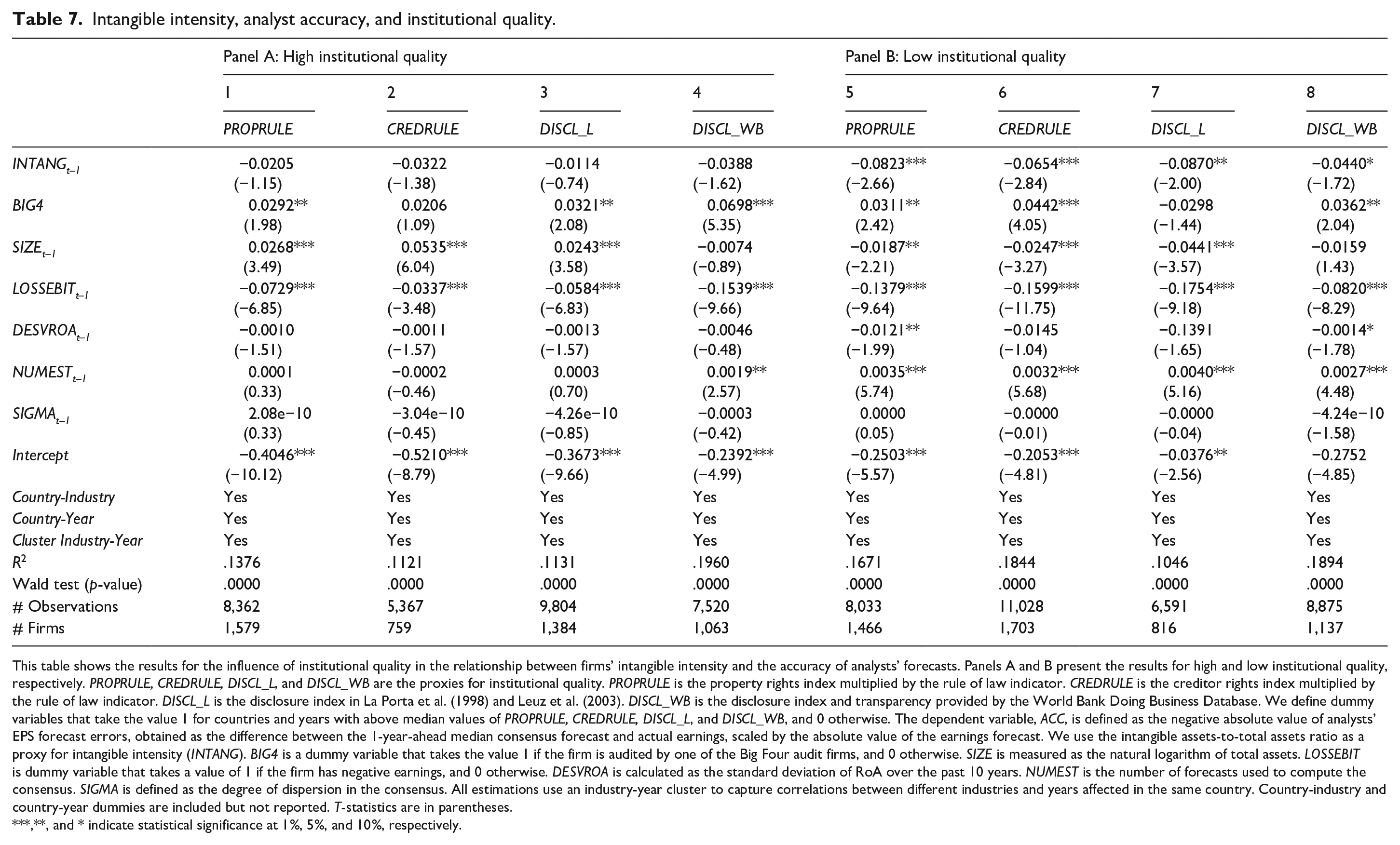
This table shows the results for the influence of institutional quality in the relationship between firms’ intangible intensity and the accuracy of analysts’ forecasts. Panels A and B present the results for high and low institutional quality, respectively. PROPRULE, CREDRULE, DISCL_L, and DISCL_WB are the proxies for institutional quality. PROPRULE is the property rights index multiplied by the rule of law indicator. CREDRULE is the creditor rights index multiplied by the rule of law indicator. DISCL_L is the disclosure index in La Porta et al. (1998) and Leuz et al. (2003). DISCL_WB is the disclosure index and transparency provided by the World Bank Doing Business Database. We define dummy variables that take the value 1 for countries and years with above median values of PROPRULE, CREDRULE, DISCL_L, and DISCL_WB, and 0 otherwise. The dependent variable, ACC, is defined as the negative absolute value of analysts’ EPS forecast errors, obtained as the difference between the 1-year-ahead median consensus forecast and actual earnings, scaled by the absolute value of the earnings forecast. We use the intangible assets-to-total assets ratio as a proxy for intangible intensity (INTANG). BIG4 is a dummy variable that takes the value 1 if the firm is audited by one of the Big Four audit firms, and 0 otherwise. SIZE is measured as the natural logarithm of total assets. LOSSEBIT is dummy variable that takes a value of 1 if the firm has negative earnings, and 0 otherwise. DESVROA is calculated as the standard deviation of RoA over the past 10 years. NUMEST is the number of forecasts used to compute the consensus. SIGMA is defined as the degree of dispersion in the consensus. All estimations use an industry-year cluster to capture correlations between different industries and years affected in the same country. Country-industry and country-year dummies are included but not reported. T-statistics are in parentheses.
**, and * indicate statistical significance at 1%, 5%, and 10%, respectively.
The economic significance of the relationship between intangible intensity and analyst accuracy in countries with different levels of institutional quality is also worth checking. Taking, for instance, the results in Column 5 of Table 7, it can be seen that an increase of one standard deviation (0.1847) in the intangible assets-to-total assets ratio (INTANG) of firms in institutionally less developed countries proxied by PROPRULE would result in a 5.55% reduction in accuracy levels. In other words, the lower information asymmetry traditionally associated with institutionally more developed environments has the potential to compensate for the negative effect of intangible assets on analyst forecast accuracy.
Intangible intensity and analyst accuracy: implications on the cost of equity
In this section, we shed additional light on the potential implications of our basic analysis from the firm-level perspective. Specifically, we empirically explore the extent to which the relationship between intangible intensity and the level of analyst accuracy could affect the cost of access to financial resources for firms. Our empirical strategy calls for a dual approach. First, we run a mediation test (Hayes, 2009, 2013; Shrout, 2011) to check the extent to which the lower analyst forecast accuracy observed for high intangible firms may act as a channel through which the cost of equity may be influenced. Next, we take the residual component of the regression explaining analyst accuracy as an explanatory variable for the cost of equity. The idea is to demonstrate that the part of accuracy of analyst forecasts not explained by intangible intensity still affects the cost of equity. This would enable us to assess the impact of the reduction in analyst forecast accuracy in terms of the cost of equity for firms.
For these empirical analyses, we construct two measures for the cost of equity based on earnings forecast data. First, following Easton (2004), we take abnormal earnings growth as constant after year t + 1 and future dividends as equal to zero. We therefore compute the cost of equity as the square root of the difference between the EPS consensus forecast for fiscal year y and the 2-year-ahead EPS consensus forecast, divided by the asset price. As an alternative, and following Cheng et al. (2006), we estimate the cost of equity deriving from expected earnings growth valuation models. Cheng et al.’s model also includes forecasted earnings per share for 1 and 2 years ahead together with a perpetual growth rate for the firms. 15
Mediation test
Previous research has suggested that information plays an important role in determining the cost of equity for firms (Francis et al., 2005; Hail, 2002; Leuz & Verrecchia, 2000 among others). W. P. He et al. (2013) confirm that information asymmetry does increase a firms’ cost of equity. This is consistent with findings in Easley and O’Hara (2004) who stated that information risk tends to increase a firm’s cost of equity. This relationship has been analyzed in depth from the perspective of firm disclosure practices. Francis et al. (2005) find that higher voluntary disclosure levels in firms belonging to industries with greater external financing lead to a reduction in the cost of equity. In accordance with this line of research, Leuz and Verrecchia (2000) and Hail (2002) provide evidence of a negative association between disclosure levels, as a mechanism to reduce information asymmetries, and the cost of capital. While previous literature examines the relationships between information and the cost of capital by investigating firm disclosure practices and the required rate of return, our study focuses on the effect of information asymmetry proxied by intangible intensity. Given the higher degree of information asymmetry in firms with large proportions of intangible assets, it would be here that one should expect to find a higher increment in the cost of equity, therefore, clearly evidencing the basic negative relationship between intangible intensity and analyst accuracy.
Reports by financial analysts, in their capacity as sophisticated agents who are better informed than the average investor, can be valuable in improving the credibility of earnings forecasts and thereby reducing information risk. W. P. He et al. (2013) find that earnings forecast dispersion increases the ex-ante cost of equity, while analyst coverage tends to decrease the rate of return demanded by investors. The main explanation, as the authors conclude, is that greater dispersion in earnings forecasts is an indication of information uncertainty, which triggers an increase in the rate of return demanded by investors. However, higher analyst coverage leads to greater information disclosure, which actually reduces the cost of equity. Given that analysts are important drivers of information, helping market participants to reduce the degree of information asymmetry among firms’ stakeholders and to properly value securities, we examine the relationship between intangible intensity and the firms’ cost of equity, completing this analysis with the potential mediator role played by analyst activity.
The results of the mediation model for all the firms of our sample are shown in Panel A of Table 8. We report the direct, indirect, and total effects of the mediation test, respectively. In Column 1, we follow Easton (2004) for the calculation of the measure of cost of equity. Column 2 reports the results using the cost-of-equity proxy defined by Cheng et al. (2006).
The effect of intangible intensity and analyst accuracy on the cost of equity: mediation and residuals analyses.
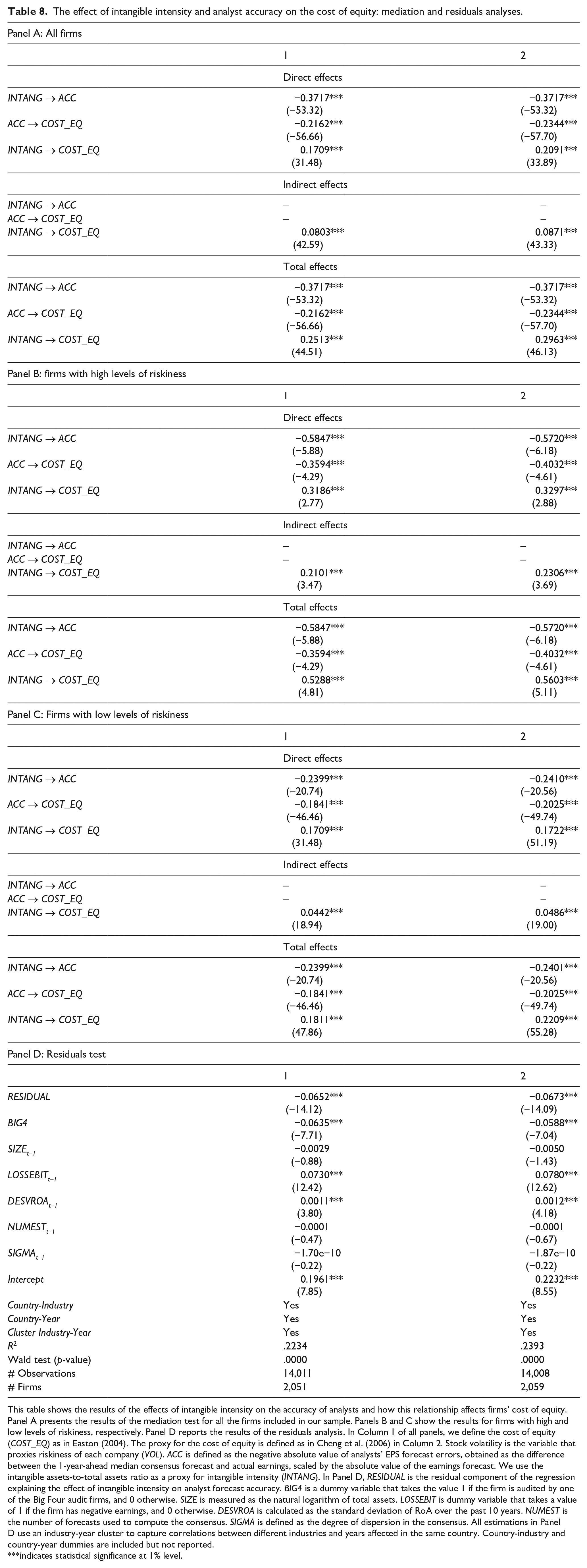
This table shows the results of the effects of intangible intensity on the accuracy of analysts and how this relationship affects firms’ cost of equity. Panel A presents the results of the mediation test for all the firms included in our sample. Panels B and C show the results for firms with high and low levels of riskiness, respectively. Panel D reports the results of the residuals analysis. In Column 1 of all panels, we define the cost of equity (COST_EQ) as in Easton (2004). The proxy for the cost of equity is defined as in Cheng et al. (2006) in Column 2. Stock volatility is the variable that proxies riskiness of each company (VOL). ACC is defined as the negative absolute value of analysts’ EPS forecast errors, obtained as the difference between the 1-year-ahead median consensus forecast and actual earnings, scaled by the absolute value of the earnings forecast. We use the intangible assets-to-total assets ratio as a proxy for intangible intensity (INTANG). In Panel D, RESIDUAL is the residual component of the regression explaining the effect of intangible intensity on analyst forecast accuracy. BIG4 is a dummy variable that takes the value 1 if the firm is audited by one of the Big Four audit firms, and 0 otherwise. SIZE is measured as the natural logarithm of total assets. LOSSEBIT is dummy variable that takes a value of 1 if the firm has negative earnings, and 0 otherwise. DESVROA is calculated as the standard deviation of RoA over the past 10 years. NUMEST is the number of forecasts used to compute the consensus. SIGMA is defined as the degree of dispersion in the consensus. All estimations in Panel D use an industry-year cluster to capture correlations between different industries and years affected in the same country. Country-industry and country-year dummies are included but not reported.
indicates statistical significance at 1% level.
We find both direct and indirect effects of intangible intensity on the cost of equity. Both the direct and indirect effects (mediated by analyst forecasting accuracy) are positive and statistically significant at conventional levels. This is consistent with the claim that higher levels of intangible assets increase the cost of financial resources for firms. Regarding the indirect effect, our results provide evidence of the mediating role played by the accuracy of analyst forecasts. 16 It emerges that analyst accuracy acts as a mechanism through which the higher levels of (information) risk associated with intangible investments are priced into the cost of equity. Moreover, and according to our main empirical findings, we provide evidence to show that higher proportions of balance sheet intangibles are negatively correlated with the accuracy of analyst forecasts.
However, one concern here could be that the overall risk of the firm is not accounted for and the mediator role of analyst accuracy may not be equally relevant for all types of firms. Hence, in Panels B and C of Table 8, we demonstrate that the effect of intangible intensity on the cost of equity mediated through analyst accuracy still holds after controlling for global risk level of the firms. To do this, in Panel B, we present the results for the subsample of firms with a level of stock volatility higher than the 75th percentile. Results in Panel C are reported for those firms whose level of stock volatility is lower the 25th percentile. As can be seen, the results of the mediation test across subsamples of firms with different global risk are consistent to those presented in Panel A for the entire sample.
Residual component
According to the basic results shown, it can be assumed that the larger the proportion of intangible assets in the balance sheet of the firm, the less accurate the earnings forecasts. Consistent with previous literature, moreover, analysts are shown to be important drivers of information, helping market participants to reduce the degree of information asymmetry and to properly value securities (Brennan et al., 1993; Francis & Soffer, 1997; Givoly & Lakonishok, 1979; Hong et al., 2000; Lys & Sohn, 1990). Hence, we specifically examine whether, once the impact of intangible intensity is removed, analyst forecasting accuracy still significantly reduces the average cost of equity.
Our empirical strategy combines a residual component analysis with panel data estimators. We regress our analyst accuracy variable on intangible intensity while controlling for the other relevant firm-characteristic factors (BIG4, SIZE, LOSSEBIT, DESVROA, SIGMA, and NUMEST). We obtain the residual component of this equation, which will be included as an additional explanatory variable for the equation explaining the cost of equity. The structural equation to be estimated is specified as follows:
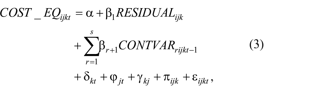
where the dependent variable is the cost of equity for firm i, in industry j, and country k, at period t, following Easton (2004) and Cheng et al. (2006).
In Panel D of Table 8, we show the empirical evidence for this analysis. Again, in Column 1, we present the results using the cost of equity measure proposed by Easton (2004). In Column 2, we show the empirical findings obtained when the cost of equity proxy is that defined by Cheng et al. (2006). In both cases, we obtain a negative and statistically significant coefficient for the RESIDUAL variable, indicating that the part of analyst forecast accuracy not explained by intangible intensity still reduces the cost of equity. This result is consistent with previous literature where it has been demonstrated that the accuracy of earnings forecasts provides a mechanism through which information asymmetries between firm insiders and outsiders are reduced (DeFond & Hung, 2007; Easley & O’Hara, 2004; Hong et al., 2000). Overall, our findings appear to indicate that, at least to some extent, it is necessary to consider that higher cost of equity could be due to intangible intensity making analysts’ assessment of the underlying firms’ financials more difficult.
Robustness tests
In further analysis, we perform additional robustness checks on our results. First, we apply alternative estimation methods. Specifically, we apply a two-stage Heckman (1979) procedure to address potential sample selection bias. We also replicate our basic set of results using a dynamic panel GMM estimator. We then check whether our results still hold after controlling for stock characteristics, identified in the traditional literature as indicators of hard-to-value and difficult-to-arbitrage (HVDA) firms. Next, we check whether successive changes in accounting standards during our time-window of interest brought about changes in corporate investment patterns and analyst behavior. We also test the extent to which specific regulatory and transparency requirements affecting some industrial sectors may play a role in explaining the relationship between intangible intensity and analyst accuracy. Finally, we check the robustness of our empirical findings to account for crisis years and alternative measures of intangible intensity.
Alternative estimation methods: two-stage Heckman (1979) and GMM estimator
The decision by analysts to release information and forecasts for a given firm is probably not taken randomly. It may be motivated by certain firm characteristics which, in turn, determine the accuracy of the earnings forecast. Given this econometric concern, we test whether our results hold when the decision of a financial analyst to start following a firm is considered, not as fully exogenous, but partially driven by specific firm characteristics. In such a setting, where observations are not randomly assigned to different groups, panel data regressions may not provide consistent estimates. Hence, we perform a two-stage Heckman (1979) regression analysis that controls for sample selection bias and endogeneity between the analyst’s decision and firm characteristics.
We specify a first-stage probit regression, where the dependent variable is a dichotomous variable that takes the value 1 if a firm is followed by financial analysts during a particular period, and 0 otherwise (ANALYSTS). The Heckman (1979) method enables us to estimate λ, which is equivalent to the inverse Mill’s ratio of the financial analyst’s decision whether or not to follow a firm. As explanatory variables, we consider the whole set of variables used to explain analyst forecast accuracy in the second stage, plus an exogenous variable to identify the first-stage decision. To obtain a consistent estimate of a firm’s probability of being followed by financial analysts, we must remove from the outcome equation at least one of the exogenous variables in the selection equation. Specifically, the first-stage equation must include an additional exogenous variable to explain the choice of the financial analyst without being directly related to the accuracy of the forecast. Following previous literature explaining the underlying motives of the analyst’s decision to start following a firm (Bhushan, 1989; Marston, 1997), we use the book-to-market ratio (BTM) as an inverse proxy of growth opportunities. In line with previous research, our intuition is that BTM affects the financial analyst’s decision to start issuing earnings forecasts for a firm but is not directly related to the accuracy of the released information. 17
The second-stage estimation is a panel data regression model, where the dependent variable is analyst forecast accuracy (ACC). In this second specification, we include the λ, the inverse Mills ratio, from the first stage as an additional independent variable for analyst accuracy. In Columns 1 to 4 of Table 9, we present the results of the Heckman’s two-stage model. Columns 1 and 3 report the first- and second-stage estimates obtained without restricting our sample of firm-year observations to firms with the firm-level control variables, while Columns 2 and 4 do include the firm-level controls. BTM appears as a significant explanatory variable in the first-stage probit regressions suggesting that firms with higher growth opportunities are the preferred choices of financial analysts.
Intangible intensity and analyst accuracy: alternative estimation methods.
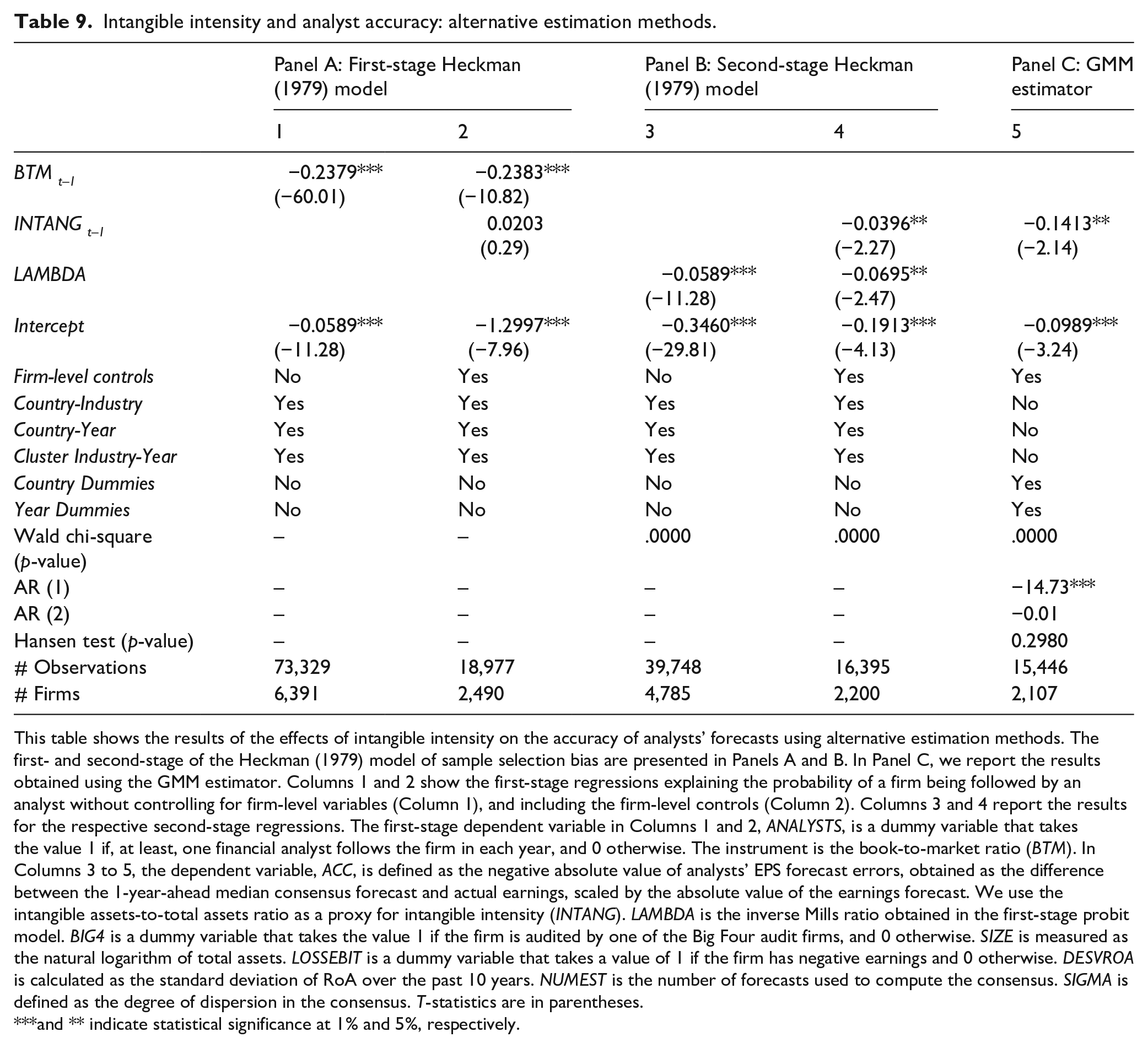
This table shows the results of the effects of intangible intensity on the accuracy of analysts’ forecasts using alternative estimation methods. The first- and second-stage of the Heckman (1979) model of sample selection bias are presented in Panels A and B. In Panel C, we report the results obtained using the GMM estimator. Columns 1 and 2 show the first-stage regressions explaining the probability of a firm being followed by an analyst without controlling for firm-level variables (Column 1), and including the firm-level controls (Column 2). Columns 3 and 4 report the results for the respective second-stage regressions. The first-stage dependent variable in Columns 1 and 2, ANALYSTS, is a dummy variable that takes the value 1 if, at least, one financial analyst follows the firm in each year, and 0 otherwise. The instrument is the book-to-market ratio (BTM). In Columns 3 to 5, the dependent variable, ACC, is defined as the negative absolute value of analysts’ EPS forecast errors, obtained as the difference between the 1-year-ahead median consensus forecast and actual earnings, scaled by the absolute value of the earnings forecast. We use the intangible assets-to-total assets ratio as a proxy for intangible intensity (INTANG). LAMBDA is the inverse Mills ratio obtained in the first-stage probit model. BIG4 is a dummy variable that takes the value 1 if the firm is audited by one of the Big Four audit firms, and 0 otherwise. SIZE is measured as the natural logarithm of total assets. LOSSEBIT is a dummy variable that takes a value of 1 if the firm has negative earnings and 0 otherwise. DESVROA is calculated as the standard deviation of RoA over the past 10 years. NUMEST is the number of forecasts used to compute the consensus. SIGMA is defined as the degree of dispersion in the consensus. T-statistics are in parentheses.
and ** indicate statistical significance at 1% and 5%, respectively.
In the second-stage model specifications, the coefficient of λ is negative and statistically significant, which suggests a negative correlation between the error terms in the selection and primary equations. These findings indicate that unobserved factors that motivate a financial analyst to start following a firm need to be considered to avoid selection bias. The negative and statistically significant coefficient of INTANG in the estimate reported in Column 4 confirms that, after controlling for potential sample selection bias and endogeneity of the financial analyst’s decision, higher intangible intensity significantly undermines the accuracy of analyst forecasts.
The second alternative econometric method to be applied is the GMM estimator. The specific aim is to address three relevant econometric issues potentially affecting our basic study of the relationship between intangible intensity and analyst accuracy: (1) unobservable firm-level heterogeneity; (2) autoregressive effects in the data describing the behavior of the dependent variables; and (3) potential endogeneity in the explanatory variables when firm-level data are used. The panel estimator controls for potential endogeneity by using instruments based on lagged values of the explanatory variables. Specifically, we apply a two-step GMM system and specify the robust estimator of the variance–covariance matrix. This is a variant of the GMM estimation method originally proposed by Arellano and Bond (1991) and Arellano and Bover (1995) and improved by Blundell and Bond (1998) that combines the difference equation with a level equation to form a system of equations for estimation purposes. The GMM system estimator exhibits higher levels of both consistency and efficiency than the difference-in-difference estimator proposed by Arellano and Bond (1991) and enables the use of time-invariant (or highly persistent) variables in our specifications. The validity of the GMM system estimator approach rests on two testable assumptions. First, for the instruments to be valid, they need to be uncorrelated with the error term. We use the Sargan statistic of over-identifying restrictions to test this assumption (where statistically insignificant values confirm the validity of the instruments). Second, the GMM system estimator requires stationarity in the post-instrumentation error terms. This implies the absence of second-order serial correlation in the first-difference residual. We employ the m2 statistic developed by Arellano and Bond (1991) to test for a lack of second-order serial correlation in the first-difference residual. An insignificant m2 statistic indicates that the model is correctly specified.
In Column 5 of Table 9, we report the results of the GMM procedure. The results obtained allow us to confirm that the negative relationship between intangible intensity and the accuracy of analyst forecasts holds after controlling for potential endogeneity among all the explanatory variables and the potential dynamics of analyst accuracy.
HVDA firms, intangible intensity, and analyst accuracy
Previous literature has documented the role of specific firm-level characteristics which make it possible to identify firms and stocks as HVDA. This particular type of firm is, by definition, more sensitive to potential cognitive bias and thus more difficult to value (Baker & Wurgler, 2006). HVDA firms are classified specifically by their level of stock volatility, market capitalization, dividends, and BTM ratio. The grounds for identifying intangible-intensive firms as HVDA firms are that intangible intensity characteristics, in conjunction with accounting regulations, complicate firm valuation (Barth et al., 2001; Hall, 2002). As previously discussed, there are also reasons to expect higher uncertainty about firm value in these than in other firms, as well as the presence of conditions that sustain stakeholder asymmetry (Aboody & Lev, 2000; Nagar, 1999; Verrecchia, 2001).
Thus, it might be useful to proceed directly to determining whether the two sets of firms (HVDA firms and firms with higher levels of intangible assets) are fundamentally similar or sufficiently different to preclude the possibility of applying existing research findings indistinctly to either. To answer this question, firms are sorted annually for the sample period based on the intangibility measure (INTANG) into 10 portfolios and values of the HVDA firm proxies (VOL or PCA 18 ) are computed. An analysis of variance (ANOVA) test is then run to test for significant between-group differences. Panel A of Table 10 summarizes the results from the parametric and non-parametric ANOVAs. Given that the analysis is performed annually, we list the maximum, minimum and average p-values, and the 10th and 90th percentiles. The fact that we find no between-group difference in means confirms that our HVDA and intangible intensity measures describe significantly different groups of firms. 19 Parametric and non-parametric tests also verified the robustness of the results.
Intangible intensity, analyst accuracy, and HVDA firms.
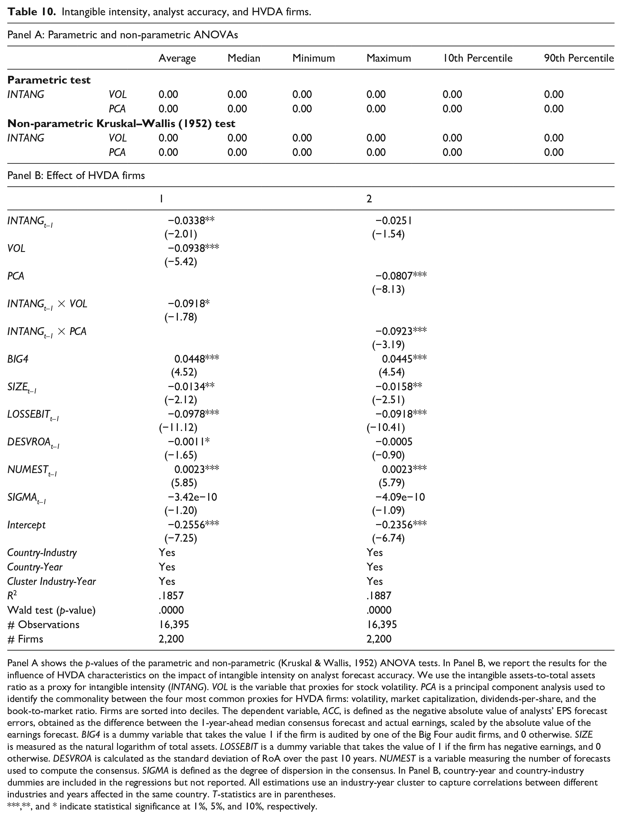
Panel A shows the p-values of the parametric and non-parametric (Kruskal & Wallis, 1952) ANOVA tests. In Panel B, we report the results for the influence of HVDA characteristics on the impact of intangible intensity on analyst forecast accuracy. We use the intangible assets-to-total assets ratio as a proxy for intangible intensity (INTANG). VOL is the variable that proxies for stock volatility. PCA is a principal component analysis used to identify the commonality between the four most common proxies for HVDA firms: volatility, market capitalization, dividends-per-share, and the book-to-market ratio. Firms are sorted into deciles. The dependent variable, ACC, is defined as the negative absolute value of analysts’ EPS forecast errors, obtained as the difference between the 1-year-ahead median consensus forecast and actual earnings, scaled by the absolute value of the earnings forecast. BIG4 is a dummy variable that takes the value 1 if the firm is audited by one of the Big Four audit firms, and 0 otherwise. SIZE is measured as the natural logarithm of total assets. LOSSEBIT is a dummy variable that takes the value of 1 if the firm has negative earnings, and 0 otherwise. DESVROA is calculated as the standard deviation of RoA over the past 10 years. NUMEST is a variable measuring the number of forecasts used to compute the consensus. SIGMA is defined as the degree of dispersion in the consensus. In Panel B, country-year and country-industry dummies are included in the regressions but not reported. All estimations use an industry-year cluster to capture correlations between different industries and years affected in the same country. T-statistics are in parentheses.
**, and * indicate statistical significance at 1%, 5%, and 10%, respectively.
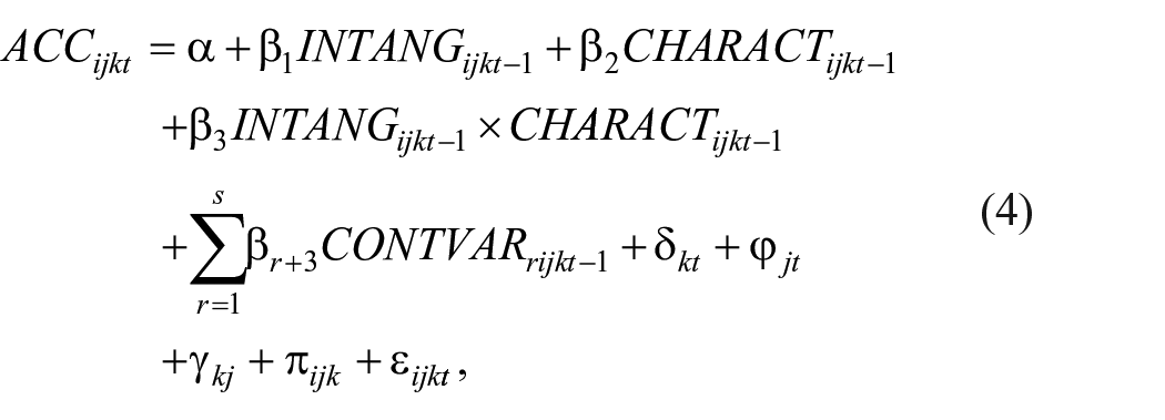
The above results enable us to state that, despite both types of firms being difficult to value, firms with high intangible intensity cannot be identified as so-called HVDA firms, and that past research findings for HVDA firms cannot therefore be directly extended to intangible-intensive firms. Thus, it is worth determining whether the observed findings for the relationship between intangible intensity and analyst accuracy still hold after controlling for the HVDA effect on accuracy (Corredor et al., 2014; Hribar & McInnis, 2012; Qian, 2009). Therefore, the model to be estimated is written as follows:
where
In addition, we find that the interaction between the two groups of firms (INTANG × CHARACT) is negative and statistically significant. This is consistent with a complementary effect between intangible intensity and the characteristics that define HVDA firms. Therefore, intangible intensity, jointly considered with other indicators of difficult valuation and arbitrage, reduces the accuracy of analyst information.
Intangible intensity, analyst accuracy, and regulations on intangible assets
Another key factor in the quality of accounting information is that of the regulatory and accounting requirements affecting intangible assets. The observation window for our sample enables us to study the effect of the implementation, in 2005, of International Financial Reporting Standards (IFRS) for European firms, which changed the treatment of intangible investments. We then extend the analysis to other changes in accounting standards, since the IFRS substantially altered the IAS 36 and IAS 38 accounting standards, and to include the IFRS 3 introduced in 2009. Thus, in this robustness section, we aim to examine whether these changes in accounting standards, which potentially affect the degrees of information asymmetry, alter analysts’ interpretation of the financials, by checking for increases or decreases in analyst accuracy. The objective of the IAS 36 (Impairment of Assets, 2004) is to establish the procedure that firms must adopt to ensure that assets are carried at no more than their recoverable amount, and to define how the recoverable amount is determined. IAS 38 (Intangible Assets, 2004) governs the recognition criteria and measurement models as well as relevant disclosures of intangible assets. Finally, IFRS 3 (Business Combinations), introduced in 2009, obliges an acquirer to recognize the identifiable intangible assets of the acquiree other than goodwill.
Financial analysts are among the major users of financial statements, as they intensively use accounting information to forecast or estimate a firm’s fundamental value (Barron et al., 2002), so an examination of how harmonization to enhance the usefulness of accounting information affects analysts in the relation with high intangible intensity is necessary. In fact, using a non-US sample, Ashbaugh and Pincus (2001) find that analyst accuracy improves after firms adopt IFRS. Lower forecast error after the adoption of IFRS because of a larger set of disclosures is also found in Hodgdon et al. (2008) and Glaum et al. (2013). In relation to the impact of IAS 38, Matolcsy and Wyatt (2006) find that capitalization of intangible assets is associated with lower earnings forecast dispersion and lower absolute earnings forecast error. André et al. (2018) score compliance with the mandatory disclosure requirements of IAS 36 and IAS 38 in European firms. They document that analysts make less dispersed forecasts and that their predictions are, in fact, more accurate. This evidence supports the argument that mandatory disclosure requirements provide insights into key accounting matters that result in more transparent financial statements.
For our specific study, we create three individual dichotomous variables that take a value of 1 if the periods are 2004–2016, 2005–2016, and 2009–2016 for the IAS rules, IFRS, and IFRS 3, respectively, and 0 otherwise. 20 The results are shown in Table 11. Columns 1, 2, and 3 show the results of the IAS, IFRS, and IFRS 3 adoption, respectively. According to these findings, the negative relationship between intangible asset intensity and analyst forecasting accuracy holds completely. However, forecast accuracy has improved for high intangible intensity firms, since the coefficient of the interaction term between the dummy variable post-adoption of the new accounting rules and intangible intensity is positive, although it is only statistically significant at conventional levels in the case of IFRS adoption. Thus, we are able to conclude that the new technical standards imposed by the IFRS accounting rules have improved the accuracy in this kind of intangible assets by enhancing disclosure requirements and, therefore, transparency. Hence, IAS/IFRS disclosure requirements have reduced information asymmetries and enhanced the ability of financial analysts to provide more accurate forecasts.
Intangible intensity, analyst accuracy, and regulations on intangible assets.
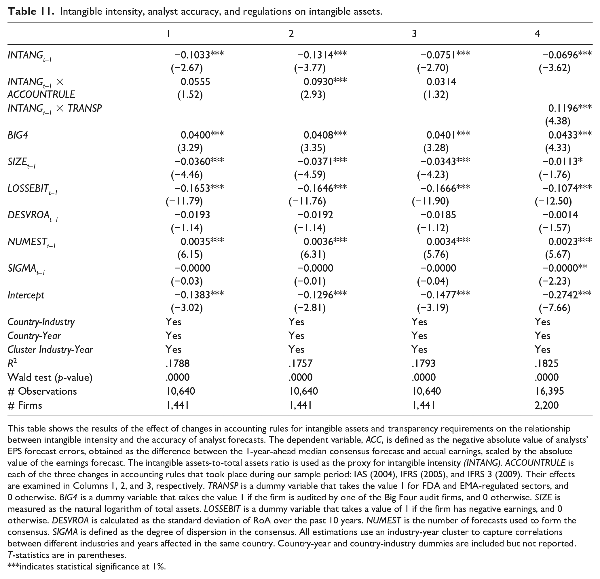
This table shows the results of the effect of changes in accounting rules for intangible assets and transparency requirements on the relationship between intangible intensity and the accuracy of analyst forecasts. The dependent variable, ACC, is defined as the negative absolute value of analysts’ EPS forecast errors, obtained as the difference between the 1-year-ahead median consensus forecast and actual earnings, scaled by the absolute value of the earnings forecast. The intangible assets-to-total assets ratio is used as the proxy for intangible intensity (INTANG). ACCOUNTRULE is each of the three changes in accounting rules that took place during our sample period: IAS (2004), IFRS (2005), and IFRS 3 (2009). Their effects are examined in Columns 1, 2, and 3, respectively. TRANSP is a dummy variable that takes the value 1 for FDA and EMA-regulated sectors, and 0 otherwise. BIG4 is a dummy variable that takes the value 1 if the firm is audited by one of the Big Four audit firms, and 0 otherwise. SIZE is measured as the natural logarithm of total assets. LOSSEBIT is a dummy variable that takes a value of 1 if the firm has negative earnings, and 0 otherwise. DESVROA is calculated as the standard deviation of RoA over the past 10 years. NUMEST is the number of forecasts used to form the consensus. SIGMA is defined as the degree of dispersion in the consensus. All estimations use an industry-year cluster to capture correlations between different industries and years affected in the same country. Country-year and country-industry dummies are included but not reported. T-statistics are in parentheses.
indicates statistical significance at 1%.
We complement our study with a further test focusing on industries subject to regulations aimed at increasing the transparency of their innovation processes. The US Food and Drug Administration (FDA), for example, is responsible for protecting and promoting public health by ensuring the safety, efficacy, and security of certain products. The EU equivalent is the European Medical Agency (EMA), whose mission it is to foster scientific excellence in the evaluation and supervision of medicines, for the benefit of the EU’s public and animal health. The FDA and EMA regulate a wide range of products, including animal and veterinary products, cosmetics, human drugs, human foods, tobacco products, and medical devices intended for human use. 21 The higher levels of transparency and supervisory requirements affecting these industries might lead us to expect a weaker relationship between intangible assets and accuracy due to the reduction in information asymmetry achieved by such regulatory measures.
To empirically test this effect, we define a dummy variable (TRANSP) that takes the value 1 for industrial sectors subject to FDA and EMA regulations, and 0 otherwise. To examine how far a specific regulation on a particular intangible asset may alter the statistical significance of our basic result on the relationship between intangible intensity and analyst accuracy, we define the interaction term between the intangible intensity proxy and the dummy for regulated industries (INTANG × TRANSP).
According to the empirical findings shown in Column 4 of Table 11, there is a positive and statistically significant coefficient on the interaction term between INTANG and TRANSP, which suggests that stricter information and transparency requirements affecting these industries also reduces information asymmetry problems, thereby removing the negative effect of intangible intensity on analyst accuracy. 22
Intangible intensity and analyst accuracy: other robustness tests
Given the increase in information asymmetry that usually accompanies periods of financial distress and in view of the serious consequences of the recent financial crisis 2007/2008, which occurred during our sample period, it might be useful to create a crisis dummy for possible inclusion as an additional control variable. By controlling for this variable, we are able to check the robustness of the estimated impact of intangible intensity on analyst accuracy. For instance, if intangible intensity is proxying for the effect of the crisis years, then, by controlling for the crisis period, we can rule out the possibility that the significant impact of intangible intensity on analyst accuracy may be due to the crisis rather than to a direct relationship between the two variables. This analysis also allows us to determine whether the crisis period has an independent impact on the level of analyst accuracy. We also check for interactions between intangible intensity and the crisis episode by creating the interaction term INTANG × CRISIS.
Following Laeven and Valencia (2018), we specifically construct two dichotomous variables to test the impact of the crisis period. First, we create a dummy which is assigned a value of 1 for the period 2007–2011 in the United States and the United Kingdom (2008–2012 in the other sample countries) and 0 for the remainder of the sample period (CRISIS1). Then, in an attempt to consider the potential impact, not only of the financial crisis but also of the sovereign debt crisis, we define another dummy variable which takes the value 1 during the period 2007–2012 in the United States and the United Kingdom (2008–2013 in France, Germany, and Spain), and 0 otherwise (CRISIS2). Columns 1 and 2 of Table 12 show the results. As can be seen, despite the significant negative impact of the financial and sovereign debt crises on analyst accuracy, the findings already reported for the association between accuracy and intangible intensity remain unaltered. This evidence confirms that intangible intensity constitutes within firms an additional source of informational asymmetry that is independent of the crisis episodes.
Intangible intensity, analyst accuracy: other robustness tests.
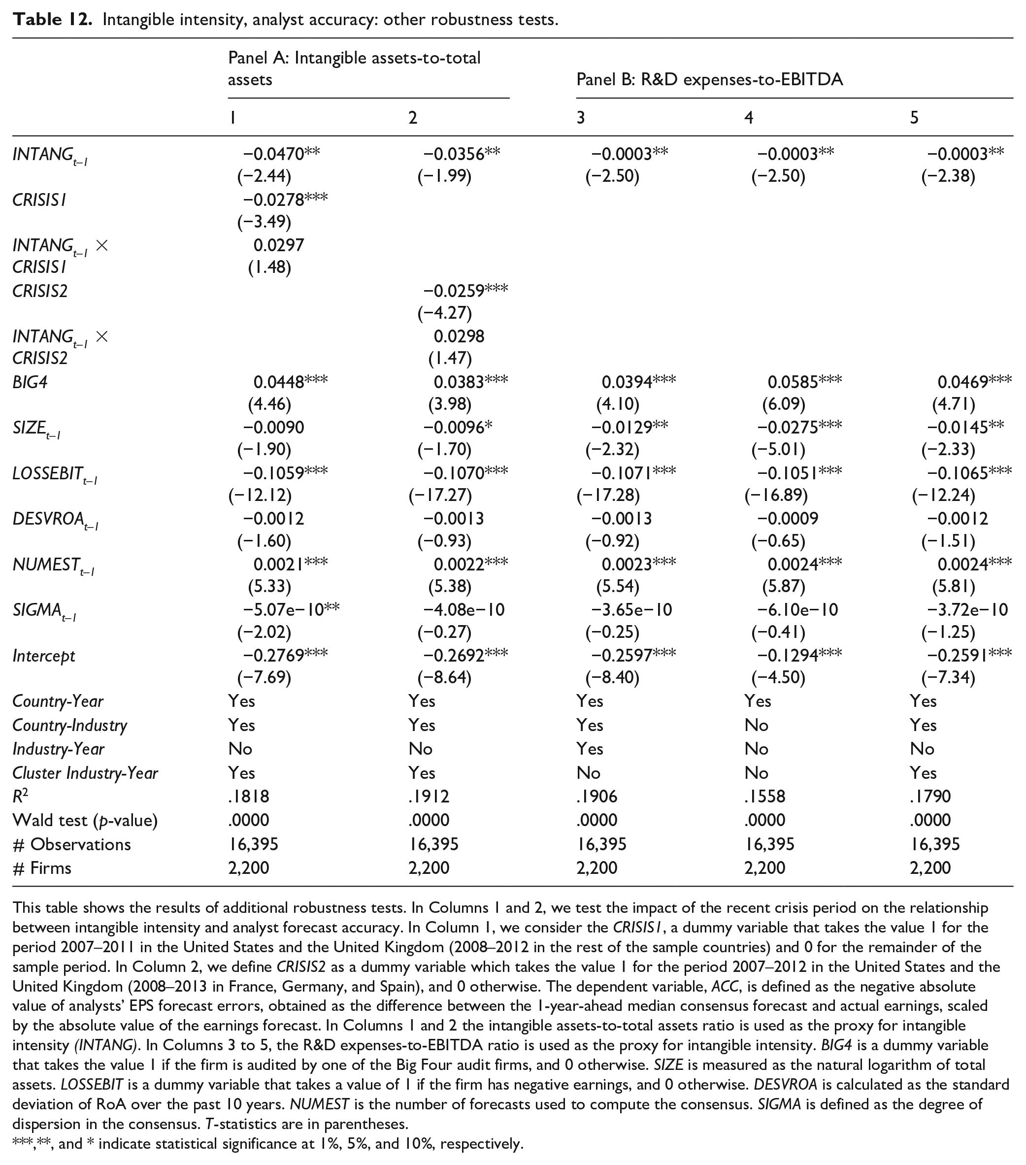
This table shows the results of additional robustness tests. In Columns 1 and 2, we test the impact of the recent crisis period on the relationship between intangible intensity and analyst forecast accuracy. In Column 1, we consider the CRISIS1, a dummy variable that takes the value 1 for the period 2007–2011 in the United States and the United Kingdom (2008–2012 in the rest of the sample countries) and 0 for the remainder of the sample period. In Column 2, we define CRISIS2 as a dummy variable which takes the value 1 for the period 2007–2012 in the United States and the United Kingdom (2008–2013 in France, Germany, and Spain), and 0 otherwise. The dependent variable, ACC, is defined as the negative absolute value of analysts’ EPS forecast errors, obtained as the difference between the 1-year-ahead median consensus forecast and actual earnings, scaled by the absolute value of the earnings forecast. In Columns 1 and 2 the intangible assets-to-total assets ratio is used as the proxy for intangible intensity (INTANG). In Columns 3 to 5, the R&D expenses-to-EBITDA ratio is used as the proxy for intangible intensity. BIG4 is a dummy variable that takes the value 1 if the firm is audited by one of the Big Four audit firms, and 0 otherwise. SIZE is measured as the natural logarithm of total assets. LOSSEBIT is a dummy variable that takes a value of 1 if the firm has negative earnings, and 0 otherwise. DESVROA is calculated as the standard deviation of RoA over the past 10 years. NUMEST is the number of forecasts used to compute the consensus. SIGMA is defined as the degree of dispersion in the consensus. T-statistics are in parentheses.
**, and * indicate statistical significance at 1%, 5%, and 10%, respectively.
Finally, in Columns 3 to 5, we use the R&D expenses-to-EBITDA ratio as a proxy for intangible intensity. In Column 3, we consider all the sets of country-year, country-industry, and industry-year fixed effects. In Column 4, the model includes only the country-year fixed effects. The results in Column 5 are the estimates from the baseline model including country-year and country-industry fixed effects and industry-year clustering. Consistently with previous results, we find a negative and statistically significant relationship between intangible intensity, proxied by the R&D expenses-to-EBITDA ratio, and the accuracy of analysts’ forecasts.
Conclusion
This article examines the relationship between firms’ intangible intensity and the accuracy of analyst forecasts. In light of the value uncertainty driven by the higher level of information asymmetry that exists between managers and external investors in this type of firm and their incentives to maintain it, our initial finding is that analyst forecast accuracy decreases significantly when a firm’s intangible intensity grows. This relationship is empirically robust to the consideration of additional firm characteristics and analyst variables as well as to different estimation techniques.
The strength of this relationship, however, varies according to the type of intangible asset. In particular, differences in the degree of tangibility associated with each type of intangible asset stress the need to control for their associated risk factors, as well as highlight the potential role of mechanisms such as accounting rules and specific regulatory requirements, to increase the level of transparency inherent to each type of investment.
The overall average negative association found between intangible intensity and analyst accuracy still holds after controlling for financial reporting quality and ownership structure. In the particular case of bank ownership, banks emerge as an effective mechanism for reducing information asymmetries in firms with higher levels of intangible intensity thereby increasing the accuracy of analyst earnings forecasts. In line with their potential for reducing information asymmetry, we also find that high-quality accounting data play a positive role in firms with larger amounts of intangible assets.
Our empirical findings are also consistent with the Law and Finance literature, which highlights the role of a country’s institutional quality in reducing information asymmetry thereby increasing the accuracy of analyst forecasts for intangible-intensive firms. Our empirical findings corroborate that, in countries with higher levels of property and creditor rights protection, stronger law enforcement, and more stringent corporate disclosure and transparency policies, the impact of intangible investments on analyst accuracy levels is less negative.
As a clear and direct implication of the negative relationship between firms’ intangible intensity and the accuracy of analyst information, our empirical analysis sheds light on the role of the accuracy of analyst forecasts as a mediating mechanism through which the higher levels of information asymmetry associated with intangible-intensive firms positively affect the corporate cost of equity.
Overall, the persistence of the negative relationship found between intangible intensity and analyst accuracy suggests that, despite the effect of various internal and external mechanisms in reducing information asymmetry, the difficulty of asset valuation is not fully removed. This, however, should not overshadow the role played by the firm’s institutional investors (particularly banks), or the strength of the country’s institutional quality, as effective mechanisms for reducing information asymmetry and, thereby, the degree of error in analyst earnings forecasts.
Footnotes
Appendix 1
Variables definitions and sources.
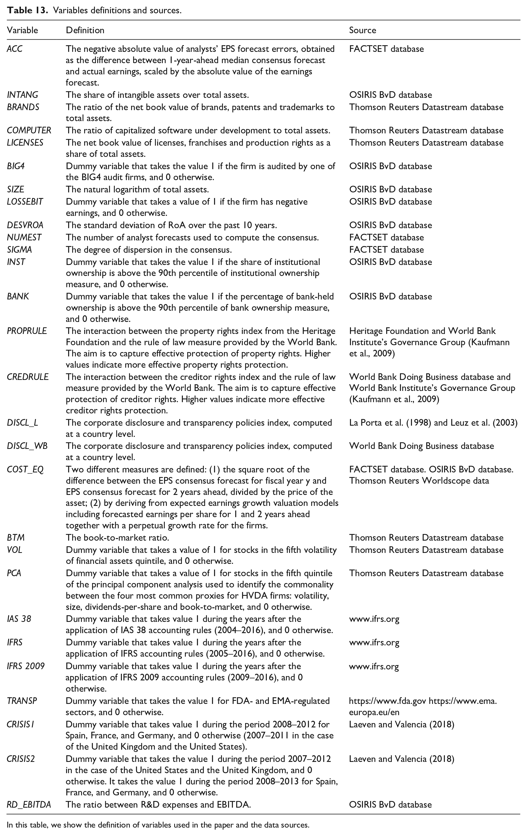
| Variable | Definition | Source |
|---|---|---|
| ACC | The negative absolute value of analysts’ EPS forecast errors, obtained as the difference between 1-year-ahead median consensus forecast and actual earnings, scaled by the absolute value of the earnings forecast. | FACTSET database |
| INTANG | The share of intangible assets over total assets. | OSIRIS BvD database |
| BRANDS | The ratio of the net book value of brands, patents and trademarks to total assets. | Thomson Reuters Datastream database |
| COMPUTER | The ratio of capitalized software under development to total assets. | Thomson Reuters Datastream database |
| LICENSES | The net book value of licenses, franchises and production rights as a share of total assets. | Thomson Reuters Datastream database |
| BIG4 | Dummy variable that takes the value 1 if the firm is audited by one of the BIG4 audit firms, and 0 otherwise. | OSIRIS BvD database |
| SIZE | The natural logarithm of total assets. | OSIRIS BvD database |
| LOSSEBIT | Dummy variable that takes a value of 1 if the firm has negative earnings, and 0 otherwise. | OSIRIS BvD database |
| DESVROA | The standard deviation of RoA over the past 10 years. | OSIRIS BvD database |
| NUMEST | The number of analyst forecasts used to compute the consensus. | FACTSET database |
| SIGMA | The degree of dispersion in the consensus. | FACTSET database |
| INST | Dummy variable that takes the value 1 if the share of institutional ownership is above the 90th percentile of institutional ownership measure, and 0 otherwise. | OSIRIS BvD database |
| BANK | Dummy variable that takes the value 1 if the percentage of bank-held ownership is above the 90th percentile of bank ownership measure, and 0 otherwise. | OSIRIS BvD database |
| PROPRULE | The interaction between the property rights index from the Heritage Foundation and the rule of law measure provided by the World Bank. The aim is to capture effective protection of property rights. Higher values indicate more effective property rights protection. | Heritage Foundation and World Bank Institute’s Governance Group (Kaufmann et al., 2009) |
| CREDRULE | The interaction between the creditor rights index and the rule of law measure provided by the World Bank. The aim is to capture effective protection of creditor rights. Higher values indicate more effective creditor rights protection. | World Bank Doing Business database and World Bank Institute’s Governance Group (Kaufmann et al., 2009) |
| DISCL_L | The corporate disclosure and transparency policies index, computed at a country level. | La Porta et al. (1998) and Leuz et al. (2003) |
| DISCL_WB | The corporate disclosure and transparency policies index, computed at a country level. | World Bank Doing Business database |
| COST_EQ | Two different measures are defined: (1) the square root of the difference between the EPS consensus forecast for fiscal year y and EPS consensus forecast for 2 years ahead, divided by the price of the asset; (2) by deriving from expected earnings growth valuation models including forecasted earnings per share for 1 and 2 years ahead together with a perpetual growth rate for the firms. | FACTSET database. OSIRIS BvD database. Thomson Reuters Worldscope data |
| BTM | The book-to-market ratio. | Thomson Reuters Datastream database |
| VOL | Dummy variable that takes a value of 1 for stocks in the fifth volatility of financial assets quintile, and 0 otherwise. | Thomson Reuters Datastream database |
| PCA | Dummy variable that takes a value of 1 for stocks in the fifth quintile of the principal component analysis used to identify the commonality between the four most common proxies for HVDA firms: volatility, size, dividends-per-share and book-to-market, and 0 otherwise. | Thomson Reuters Datastream database |
| IAS 38 | Dummy variable that takes value 1 during the years after the application of IAS 38 accounting rules (2004–2016), and 0 otherwise. | www.ifrs.org |
| IFRS | Dummy variable that takes value 1 during the years after the application of IFRS accounting rules (2005–2016), and 0 otherwise. | www.ifrs.org |
| IFRS 2009 | Dummy variable that takes value 1 during the years after the application of IFRS 2009 accounting rules (2009–2016), and 0 otherwise. | www.ifrs.org |
| TRANSP | Dummy variable that takes the value 1 for FDA- and EMA-regulated sectors, and 0 otherwise. | https://www.fda.gov https://www.ema.europa.eu/en |
| CRISIS1 | Dummy variable that takes value 1 during the period 2008–2012 for Spain, France, and Germany, and 0 otherwise (2007–2011 in the case of the United Kingdom and the United States). | Laeven and Valencia (2018) |
| CRISIS2 | Dummy variable that takes the value 1 during the period 2007–2012 in the case of the United States and the United Kingdom, and 0 otherwise. It takes the value 1 during the period 2008–2013 for Spain, France, and Germany, and 0 otherwise. | Laeven and Valencia (2018) |
| RD_EBITDA | The ratio between R&D expenses and EBITDA. | OSIRIS BvD database |
In this table, we show the definition of variables used in the paper and the data sources.
Acknowledgements
The authors thank Pablo de Andrés, Ricardo Correia, Fermín Lizárraga, Pedro Martínez Solano, Luis Muga, participants at the Fifth International Conference on Corporate Social Responsibility, Sustainability, Ethics & Governance (2018) in Santander, at the III ACEDE Workshop on Financial Economics in Murcia (2019), the Editor (Mircea Epure), and the two anonymous reviewers for the insightful and helpful comments.
Declaration of conflicting interests
The author(s) declared no potential conflicts of interest with respect to the research, authorship, and/or publication of this article.
Funding
The author(s) disclosed receipt of the following financial support for the research, authorship, and/or publication of this article: E. Ferrer acknowledges financial support from the Spanish Ministry of Economy and Competitiveness (Project ECO2016-77631-R). N. Suárez acknowledges financial support from the Spanish Ministry of Economy and Competitiveness (Project ECO2017-85356-P).