Sage Journals: Discover world-class research

Abstract

The Great Recession was the most severe economic downturn in the United States since the Great Depression. Using data from the Stanford Education Data Archive (SEDA), we describe the patterns of math and English language arts (ELA) achievement for students attending schools in communities differentially affected by recession-induced employment shocks. Employing a difference-in-differences strategy that leverages both cross-county variation in the economic shock of the recession and within-county, cross-cohort variation in school-age years of exposure to the recession, we find that declines in student math and ELA achievement were greater for cohorts of students attending school during the Great Recession in communities most adversely affected by recession-induced employment shocks, relative to cohorts of students that entered school after the recession had officially ended. Moreover, declines in student achievement were larger in school districts serving more economically disadvantaged and minority students. We conclude by discussing potential policy responses.

Keywords

Great Recession economic downturn student achievement

Introduction

December 2007 marked the onset of an 18-month economic recession that had severe and wide-ranging economic and educational consequences. During this period, now referred to as the Great Recession, the unemployment rate rose by 5 percentage points, reaching 10% by October 2009 (Evans, Schwab, & Wagner, 2019). In the wake of the Great Recession, the U.S. housing market declined dramatically, and household wealth suffered under an unprecedented shock to equity markets (Hurd & Rohwedder, 2010; Wolff, Owens, & Burak, 2011). While states and counties with the largest shares of construction employment and inflated housing stock were hardest hit by the Great Recession (Fogli, Hill, & Perri, 2015), its disproportionate effect also varied along ethnic lines. The White-Black and White-Hispanic wealth gaps increased between 2007 and 2013 (Kochhar & Fry, 2014), and negative spillovers from the economic shock onto youth outcomes, including college attendance and mental health, disproportionately affected African Americans and Hispanics (Ananat, Gassman-Pines, Francis, & Gibson-Davis, 2017; Gassman-Pines, Ananat, & Gibson-Davis, 2014).

The effect of the Great Recession on school districts was similarly pronounced, imposing constraints on state and local funding for schools (Chakrabarti & Livingston, 2013; Leachman & Mai, 2014; National Bureau of Economic Research, 2010). Evans et al. (2019) estimate that the recession reduced state and local revenues by 5%, and that educational revenues did not recover to prerecession levels until nearly 5 years after the recession. These fiscal shocks led to subsequent reductions in educational employment, with public school employment falling by 3.7%, a loss of approximately 300,000 jobs nationwide (Evans et al., 2019).

Yet, little evidence exists on the academic consequences of attending school during the Great Recession. While recent evidence documents declines in school spending nationally following the onset of the Great Recession (Evans et al., 2019), little work has examined how (and to what extent) school spending evolved differently across counties most severely affected by the recession (Shores & Steinberg, 2018). Indeed, given the importance of school inputs to student outcomes (e.g., Candelaria & Shores, 2019; Jackson, Johnson, & Persico, 2016; Lafortune, Rothstein, & Schanzenbach, 2018), the effect of the Great Recession on student academic achievement will likely depend on whether (and to what extent) students attending schools in counties differentially affected by the economic recession experienced differential declines in school spending.

In this article, we aim to fill this gap in the literature by addressing the following questions: (1) Did school spending evolve differently across schools located in counties that varied in the intensity of the economic shock of the Great Recession? (2) Was exposure to recession-induced spending declines following the onset of the Great Recession associated with declines in student achievement? (3) Were declines in student achievement following the onset of the Great Recession disproportionately concentrated in districts serving higher concentrations of low-income and minority students? This article aims to empirically assess whether (and to what extent) students who were in school during the time of the Great Recession had worse achievement outcomes than students entering school after the initial shock of the Great Recession had ended. Potential heterogeneity in changes to student achievement following the Great Recession is motivated by prior evidence that school spending has greater returns to student achievement for lower income students relative to their higher income peers (Candelaria & Shores, 2019; Jackson et al., 2016).

To address these questions, we first construct a recession intensity index that measures the extent of cross-county variation in the magnitude of the economic shock of the Great Recession. We then examine how school spending evolved in the periods before and after the onset of the Great Recession across districts located in counties that varied in the intensity of the recessionary shock to employment, and show that school spending declined significantly more in counties most adversely affected by the Great Recession—on the order of $600 per pupil per year—compared with schools located in counties least affected by the Great Recession. Notably, these differential spending declines were concentrated just in the 2-year period following the official onset of the Great Recession (i.e., the 2007–2008 to 2009–2010 period) which we define as the “exposure period”; this means that that students who attended schools located in counties differentially affected by the Great Recession were themselves exposed to differential shocks to school resources.

We then implement a difference-in-differences (DD) strategy which estimates changes in math and English language arts (ELA) achievement among students attending school during the Great Recession who were exposed to two consecutive years of annual and differential spending declines, relative to cohorts of students that entered school after this 2-year period of recession-induced spending declines. This DD strategy leverages two aspects of the data: (1) the economic shock of the recession varied across counties and (2) students in different cohorts within the same county varied in the number of years of schooling (i.e., school-age years) they were exposed to recession-induced spending declines.

We find that exposure to school spending declines following the onset of the Great Recession is associated with student math and ELA achievement declines of, on average, 0.03 standard deviations per year, which corresponds to student achievement effect sizes of approximately 0.10 sample standard deviations. The resulting achievement gap between students in counties most and least affected by the Great Recession persisted for more than 3 years after the end of the exposure period, indicating that recession-induced school spending shocks are associated with both contemporaneous and persistent declines in student achievement. Furthermore, declines in student achievement were concentrated among school districts serving more economically disadvantaged and minority students. In districts with the highest proportion of students qualifying for free/reduced-price lunch (FRPL) and in districts with the highest proportion of Black students, exposure to the recession is associated with declines in math achievement of 0.06 and 0.08 standard deviations per year, respectively (corresponding to student achievement effect sizes of 0.22 and 0.30 sample standard deviations, respectively). For ELA, we find similar results for districts with the highest proportion of Black students (0.05 standard deviations corresponding to a student achievement effect size of 0.21 sample standard deviation units). As a result, the Great Recession was associated with both aggregate declines in academic achievement and increases in achievement inequalities between poor and more economically advantaged school districts.

Notably, while we aim to isolate the recession-induced spending effect on student achievement, our empirical strategy is limited by a lack of prerecession student achievement data. This data limitation constrains us from implementing a more traditional DD strategy which would compare the achievement trajectories of cohorts of students in the periods before and after the onset of the Great Recession. We dedicate much attention in this article to explaining plausible rival hypotheses, and though we can rule out some of these, we are ultimately unable to separate the overall effect of the Great Recession on student achievement from recession-induced spending declines. Our results therefore reveal important patterns of student achievement in the wake of the Great Recession but do not provide definitive causal effects.

The article proceeds as follows. In the next section, we describe our approach for measuring county-level variation in the intensity of the Great Recession and then describe the county-level data used for the analysis. Next, we examine trends in school spending, in the pre- and postrecession periods, across counties that vary in the intensity of the Great Recession. We then discuss our empirical strategy for describing the relationship between recession-induced school resource losses during the Great Recession and student achievement declines in math and ELA. We then present our results, which include our main estimates, sensitivity analyses, and heterogeneity estimates. We conclude by discussing potential policy responses to economic shocks that adversely and heterogeneously result in student achievement declines and widening educational inequality.

Measuring Recession Intensity

We measure the intensity of the Great Recession using average annual county-level total employment data from the Quarterly Census of Employment and Wages.¹ Following Yagan (2016), we construct the following index of recession intensity:

\begin{array}{l} R e c e s s i o n_{c} = [l n (\frac{E_{c, 2010}}{E_{c, 2007}}) - \ln (\frac{E_{c, 2006}}{E_{c, 2003}})] \\ - [l n (\frac{E_{a g g, 2010}}{E_{a g g, 2007}}) - \ln (\frac{E_{a g g, 2006}}{E_{c, 2003}})] \end{array}

(1)

where $E_{c t}$ denotes the number of employed workers in county c in the Spring of academic year t, and where agg denotes total employment across the continental United States in year t. Each county’s recession intensity is measured as the change in log employment during the recessionary period (Spring 2007 to Spring 2010) relative to the county’s prerecession trend (Spring 2003 to Spring 2006). The county-specific measure of recession intensity is then normalized by subtracting the aggregate employment trend. For ease of interpretation, we convert the continuous measure of $R e c e s s i o n_{c}$ into four quartiles.

To examine whether the discretized variable $R e c e s s i o n_{c}$ accurately captures employment changes, we plot the average unemployment rate by recession intensity quartile (see Figure 1).² Figure 1 confirms that the measure of recession intensity captures meaningful geographic variation in unemployment trends beginning in Spring 2008. Note that the prerecession unemployment trends for each of the intensity quartiles are nearly identical, both in levels and in trends. Only in the postrecession period do we observe a divergence in unemployment trends by recession intensity quartile. Finally, our measure of recession intensity (i.e., $R e c e s s i o n_{c}$ ) motivates an analysis that leverages within-state, cross-county population data, since 72% of the cross-sectional variance of $R e c e s s i o n_{c}$ occurs within states. See also Appendix A, Figure A1, which displays a map of the discretized variable $R e c e s s i o n_{c}$ ³.

Figure 1.

Total expenditures, by recession intensity quartile.

Data and Sample

We construct a county-level panel data set consisting of the population of counties in the continental United States for the 2008–2009 through 2014–2015 school years. To do so, we combine data from multiple sources, including achievement information from the Stanford Education Data Archive (SEDA), demographic information from the U.S. Department of Education’s Common Core of Data (CCD) and county-level economic data from multiple sources. We describe each data source and accompanying variables below.

The SEDA data we use include estimates of average county achievement in math and ELA for nearly every county in the continental United States. These estimates are based on the roughly 300 million state accountability test scores of approximately 45 million public school students in Grades 3 through 8 during the 2008–2009 through 2014–2015 school years. Achievement data are estimated from state accountability “coarsened” proficiency data (percentages or counts of students falling into different proficiency categories, such as “Basic,” “Proficient,” and “Advanced,” which are the most commonly reported statistic available from state accountability systems), as described by Reardon, Shear, Castellano, and Ho (2017). Using a heteroskedastic ordered probit model, Reardon and colleagues show that means and standard deviations from ordered proficiency data can be recovered with little bias.

To make these test scores comparable across states (which, in almost all cases, use different standardized assessments) and across time, the achievement data are placed on a common scale using the state-level estimates from the National Assessment of Educational Progress (the “state NAEP”). This linking procedure has been described by Reardon, Kalogrides, and Ho (2017). The NAEP is a useful benchmarking tool, as it has remained relatively unchanged over time and is the same test for each state. Thus, as Reardon, Kalogrides, et al. (2017) show, it is possible to link the NAEP mean and standard deviation to the distribution of county-level achievement data estimated from state-specific standardized assessments. The SEDA data therefore provide a unique opportunity to evaluate large-scale changes in the education production function, as they allow for both within and between state comparisons of academic achievement over time. We use county-by-year-by-grade achievement scores because we leverage variation in recessionary intensity that is only available at the county level, and we use the “cohort standardized scale” because we leverage cross-cohort changes in achievement but not grade-level variation (or the linearly interpolated grade-level variation available in SEDA).⁴

To describe changes in school spending before and after the onset of the Great Recession, we construct a district-level panel data set consisting of the population of traditional public school districts in the continental United States for the 2002–2003 through 2014–2015 school years.⁵ District-level expenditure data (total, capital, and instructional) are from the CCD Local Education Agency Finance Survey (F-33). We convert all revenue and expenditure variables to real ($2013) per pupil dollars (using district enrollment totals) and eliminate outliers based on an algorithm akin to Murray, Evans, and Schwab (1998) and Berry (2007).⁶

For descriptive statistics and for heterogeneity analyses, we supplement the SEDA achievement data with district-level demographic data from the CCD that we aggregate to the county level. Demographic information includes total K–12 enrollment, total enrollment for Grades 3 to 8, proportions of Grades 3 to 8 students who are Asian, Black, Hispanic, and White, and proportions of K–12 students qualifying for FRPL. We also include the proportion of districts that are classified as urban, suburban, towns, or rural. Finally, we incorporate county-level economic data on unemployment, poverty, business establishments, and per capita income.⁷

Sample

We construct a district-to-county crosswalk and merge the school finance and SEDA achievement data. The analytic sample consists of counties with nonmissing employment, school finance, math, and ELA achievement data. This restriction yields an analytic sample that includes 2,548 counties in the United States, which is 83% of all U.S. counties for which there is achievement data, and 89,219 county-year-grade observations, which include 86% of the tested population (both traditional and charter school) in the SEDA data set.

Table 1 presents county-level descriptive statistics for the school districts included in the analytic sample. Data are shown for the 2008–2009 through 2014–2015 school years. For time-varying district characteristics, data are averaged across grades (3 through 8) and years, for the full analytic sample as well as by recession intensity quartile.

Table 1

County-Level District Characteristics, by Recession Intensity Quartile

District Characteristic	Analytic Sample	Recession Intensity Quartile
District Characteristic	Analytic Sample	Q1	Q2	Q3	Q4
Enrollment	1328.1(3826.30)	930.3 (3366.88)	1539.9 (3465.78)	1590.4 (4709.94)	1229.9 (3536.99)
Free/reduced-price lunch	0.51 (0.16)	0.57 (0.16)	0.47 (0.15)	0.50 (0.16)	0.51 (0.14)
White	0.56 (0.26)	0.46 (0.29)	0.58 (0.23)	0.56 (0.27)	0.59 (0.23)
Hispanic	0.22 (0.22)	0.29 (0.26)	0.17 (0.15)	0.22 (0.24)	0.24 (0.20)
Black	0.16 (0.17)	0.19 (0.20)	0.19 (0.16)	0.16 (0.18)	0.12 (0.13)
Asian	0.04 (0.05)	0.04 (0.06)	0.05 (0.05)	0.05 (0.04)	0.04 (0.04)
Urban	0.06	0.06	0.06	0.06	0.06
Suburban	0.23	0.14	0.30	0.28	0.15
Rural	0.52	0.60	0.47	0.48	0.55
Town	0.19	0.20	0.17	0.17	0.24
Counties	2,548	634	639	636	639

Note. Data are for the 2008–2009 through 2014–2015 school years. County-level mean (standard deviation) reported. For the geographic locale of districts (Urban, Suburban, Rural, and Town), we report the proportion of districts located in each recession intensity quartile. Enrollment is the county-level enrollment of students in Grades 3 to 8.

Table 2 presents descriptive statistics for the achievement data in our analytic sample. Data are shown for the 2008–2009 to 2014–2015 school years and are averaged across Grades 3 through 8, for the full analytic sample as well as by recession intensity quartile. Mean math and ELA achievement are precision-weighted using the inverse of the estimated standard error squared ( $1 / {\hat{σ}}^{2})$ . The use of precision weighting is motivated by the fact that the estimated standard errors for district means are, in many cases, a multiple of the estimated mean. For example, of the 89,219 county-year-grade observations available, 28,509 of those have standard errors greater than or equal to the estimated mean. Precision weighting discounts these observations. Descriptive statistics and subsequent regression models are weighted in this way, a procedure suggested by Reardon, Kalogrides, and Shores (2019).

Table 2

County-Level Achievement Outcomes, by Recession Intensity Quartile

	Analytic Sample	Recession Intensity Quartile				p From F-Test: Q4 = Q1
	Analytic Sample	Q1	Q2	Q3	Q4	p From F-Test: Q4 = Q1
Math achievement	0.02 (0.27)	−0.05 (0.28)	0.05 (0.26)	0.02 (0.28)	0.02 (0.27)	.000
English language arts (ELA) achievement	0.03 (0.24)	−0.05 (0.25)	0.06 (0.24)	0.03 (0.25)	0.05 (0.23)	.000
Counties	2,548	634	639	636	639
County * Year * Grade obs.	89,219	21,404	22,476	22,771	22,568

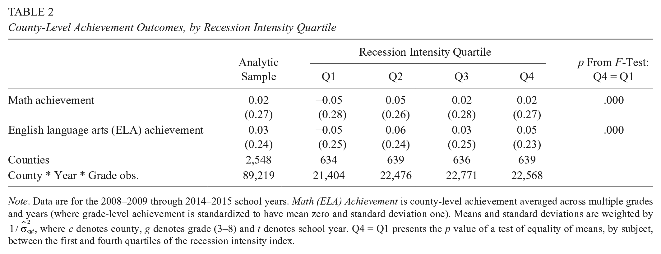
Note. Data are for the 2008–2009 through 2014–2015 school years. Math (ELA) Achievement is county-level achievement averaged across multiple grades and years (where grade-level achievement is standardized to have mean zero and standard deviation one). Means and standard deviations are weighted by $1 / {\hat{σ}}_{c g t}^{2}$ , where c denotes county, g denotes grade (3–8) and t denotes school year. Q4 = Q1 presents the p value of a test of equality of means, by subject, between the first and fourth quartiles of the recession intensity index.

School Spending Trends in the Pre- and Postrecession Periods

Figure 1 shows the trends in school expenditures, by recession intensity quartile, for the 2002–2003 through 2014–2015 school years. As has been documented elsewhere (Evans et al., 2019; Jackson, Wigger, & Xiong, 2018; Shores & Steinberg, 2018), school spending increased nationally and peaked in the 2007–2008 school year (see Figure 1). And, as we show in Figure 1, school spending increased at similar rates in the prerecession period across counties that experienced differential employment shocks following the onset of the Great Recession. Yet, in the immediate aftermath of the Great Recession (i.e., after the 2007–2008 school year), school spending evolved quite differently across schools located in counties that varied in the intensity of the recessionary shock to employment (see Figure 1, Panel B).

To directly measure how spending evolved in the pre- and postrecession periods, we calculate district-level spending trends across counties located in different recession intensity quartiles. We calculate spending trends in two ways: (1) the average annual change in district-level spending (i.e., mean spending change) and (2) the average annual rate of change in spending (i.e., spending slope).

First, we calculate the annual change in district-level spending as:

Δ S p e n d i n g_{d t} = S p e n d i n g_{d t} - S p e n d i n g_{d, t - 1},

(2)

where $S p e n d i n g_{d t}$ is per pupil expenditure (real $2013) in district d in school year t, and ∆ $S p e n d i n g_{t}$ ∈ { $Δ 2004, Δ 2005, Δ 2006, \dots, Δ 2015}$ . Then, we estimate the average annual change in district-level spending, by recession intensity quartile, as follows:

Δ S p e n d i n g_{d t} = β_{0} + β^{q} (\sum_{q = 1}^{Q} R e c e s s i o n_{i}^{q}) + ε_{d t},

(3)

where ∆ $S p e n d i n g_{d t}$ is the annual change in per pupil expenditures (real $2013) in district d (located in county i and recession intensity quartile q) in school year t and $R e c e s s i o n_{i}^{q}$ is the measure of recession intensity for county i (as described in Equation 1), which we convert into q quartiles (recession intensity Quartile 1 is the omitted reference category). We cluster standard errors at the county level (the level of recession intensity). The coefficient $β^{q}$ estimates the average annual change in district-level spending in recession intensity quartile q compared with recession intensity Quartile 1. Given the observed expenditure trends (see Figure 1, Panel B), we estimate Equation (3) separately for the following time periods: Δ2004 to Δ2008 (2002–2003 to 2007–2008); Δ2009 to Δ2010 (2007–2008 to 2009–2010); Δ2011 to Δ2013 (2009–2010 to 2012–2013); and Δ2014 to Δ2015 (2012–2013 to 2014–2015).

Next, we estimate the average annual rate of change in spending (i.e., the spending slope) by amending Equation (3) as follows:

\begin{array}{l} S p e n d i n g_{d t} = β_{0} + β^{q} (\sum_{q = 1}^{Q} R e c e s s i o n_{i}^{q} * T i m e_{t}) \\ + T i m e_{t} + μ_{d t}, \end{array}

(4)

where $S p e n d i n g_{d t}$ is per pupil expenditures (real $2013) in district d in school year t and the variable $T i m e_{t}$ is a linear time trend; all other variables are defined as in Equation (3). In Equation (4), the coefficient $β^{q}$ estimates the average annual rate of change in district-level spending (i.e., the spending slope) in recession intensity quartile q compared with the spending slope among districts in recession intensity Quartile 1. Like Equation (3), we estimate Equation (4) separately for distinct pre- and postrecession periods based on observed spending trends in Figure 1.

Table 3 summarizes these descriptive results (Table A1 summarizes spending trends in the pre- and postrecession periods separately for instructional and capital expenditures). In the 2002–2003 through 2007–2008 period—the fiscal years leading up to the official onset of the Great Recession in December 2007⁸—we find little evidence of differential spending across recession intensity quartiles, with the exception of a modest slope difference—$96.9 per pupil—among recession intensity Quartile 4 districts (relative to recession intensity Quartile 1 districts). This result confirms visual evidence from Figure 1 (Panel B); namely, districts located in counties most severely affected by the Great Recession experienced greater spending growth compared with districts in counties least adversely affected in the years prior to the onset of the Great Recession.

Table 3

Estimated Annual Change in Total Expenditures, by Time Period and Recession Intensity Quartile

	Time Period
	Δ2004 to Δ2008	Δ2009 to Δ2010	Δ2011 to Δ2013	Δ2014 to Δ2015
Panel A: Average annual change in spending
RI^{q = 2}	53.81 (42.94)	10.19 (66.59)	91.45 (67.37)	94.72 (83.09)
RI^{q = 3}	23.72 (48.09)	−333.83*** (74.04)	78.12 (63.35)	74.54 (82.51)
RI^{q = 4}	50.08 (43.43)	−567.22*** (71.68)	1.99 (64.79)	−32.60 (83.53)
	Time Period
	2003 to 2008	2008 to 2010	2010 to 2013	2013 to 2015
Panel B: Average annual rate of change in spending
RI^{q = 2}	69.20* (39.16)	20.83 (67.86)	95.08 (62.76)	73.48 (89.70)
RI^{q = 3}	34.04 (44.84)	−320.05*** (73.95)	85.85 (60.75)	41.40 (90.95)
RI^{q = 4}	96.87** (39.17)	−577.57*** (72.45)	19.65 (63.14)	−67.44 (90.13)
Counties	2,541	2,539	2,538	2,547
County * Year obs.	69,086	34,472	45,564	35,708

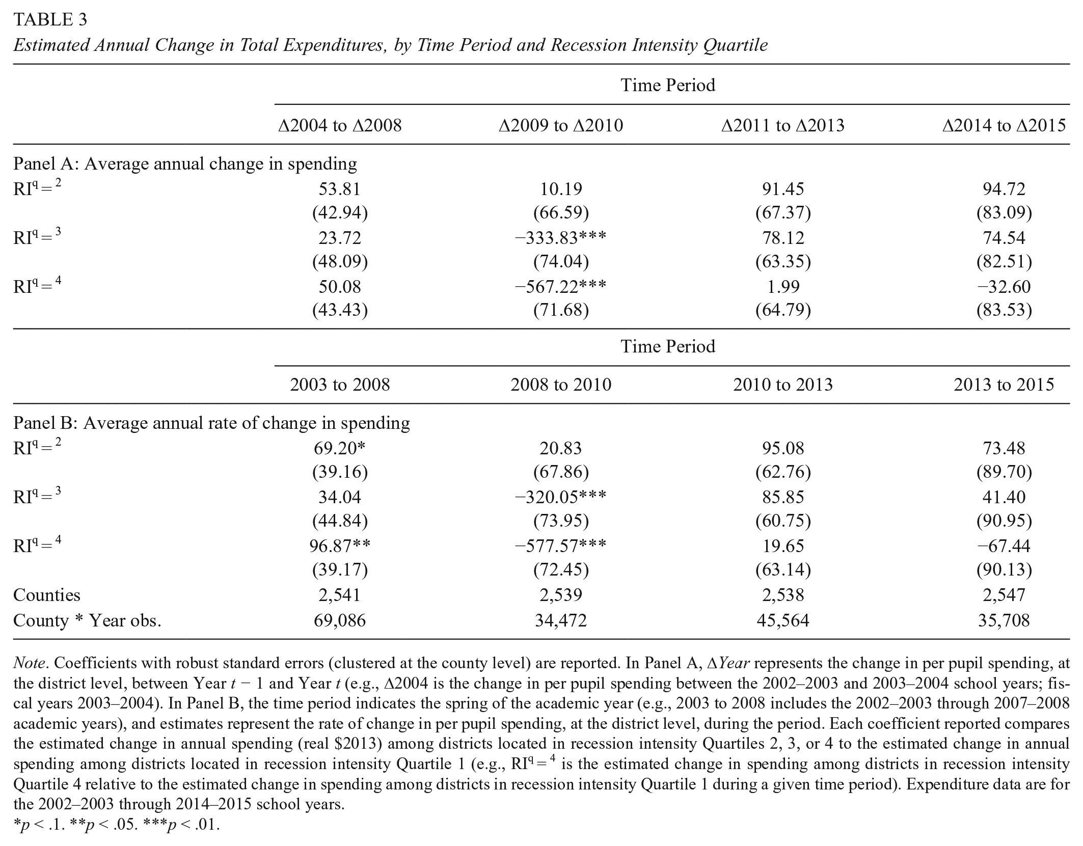
Note. Coefficients with robust standard errors (clustered at the county level) are reported. In Panel A, ΔYear represents the change in per pupil spending, at the district level, between Year t − 1 and Year t (e.g., Δ2004 is the change in per pupil spending between the 2002–2003 and 2003–2004 school years; fiscal years 2003–2004). In Panel B, the time period indicates the spring of the academic year (e.g., 2003 to 2008 includes the 2002–2003 through 2007–2008 academic years), and estimates represent the rate of change in per pupil spending, at the district level, during the period. Each coefficient reported compares the estimated change in annual spending (real $2013) among districts located in recession intensity Quartiles 2, 3, or 4 to the estimated change in annual spending among districts located in recession intensity Quartile 1 (e.g., RI^{q = 4} is the estimated change in spending among districts in recession intensity Quartile 4 relative to the estimated change in spending among districts in recession intensity Quartile 1 during a given time period). Expenditure data are for the 2002–2003 through 2014–2015 school years.

p < .1. **p < .05. ***p < .01.

Yet, following the official onset of the Great Recession, we find significant and substantive annual spending differences across recession intensity quartiles that were concentrated in the 2007–2008 through 2009–2010 period (i.e., Δ2009–Δ2010). Among recession intensity Quartile 4 districts, annual spending declined by approximately $570 per pupil (or approximately $1,140 per pupil over this period), relative to recession intensity Quartile 1 districts. Relative to instructional spending, capital spending declined the most during the exposure period, approximately $800 per pupil cumulatively, suggesting schools prioritized instructional spending in the face of fiscal shocks (see Table A1). Notably, these estimated spending losses (total, capital, and instructional) were monotonic; among recession intensity Quartile 3 districts, annual total spending declined by approximately $330 per pupil (or approximately $660 per pupil over the exposure period), relative to recession intensity Quartile 1 districts. We find no differential change in spending between recession intensity Quartile 2 and recession intensity Quartile 1 districts, those districts least adversely affected by the Great Recession.

Though spending declined among all recession intensity quartiles between the 2010 and 2013 period (see Figure 1), we find no differential change in spending across quartiles during this period (i.e., Δ2011–Δ2013 period; see Tables 3 and A1). Furthermore, during the recovery period, as spending increased among all recession intensity quartiles between years 2013 and 2015 (i.e., Δ2014–Δ2015 period), we again find no differential change in spending across quartiles (see Tables 3 and A1). Taken together, these results indicate that the economic shock of the Great Recession manifested in significant and substantive spending declines among schools located in counties most adversely affected by the Great Recession, and that these differential spending changes were concentrated just in the period following the official onset of the Great Recession—the 2008–2010 school years (Δ2009–Δ2010).

Assigning Cohorts to the Exposure Period

In the preceding section, we documented the differential spending declines among counties with different recession-induced local labor market shocks in the immediate aftermath of the Great Recession (i.e., the 2008–2010 period). This means that students whose schools were located in counties differentially affected by the Great Recession were themselves exposed to differential changes to school resources. In light of evidence that changes to school spending affect student achievement outcomes (see, e.g., Candelaria & Shores, 2019; Jackson et al., 2016; Lafortune et al., 2018; Neilson & Zimmerman, 2014), we designate the 2008–2010 period (Δ2009–Δ2010) as the exposure period.⁹ We expect that differential exposure to recession-induced changes to school spending will be correlated with differential declines in student achievement outcomes.

The SEDA provides county-level and cohort-specific test scores that can be linked to this exposure period. In Table A2, we define the 12 cohorts, based on the school year of kindergarten entry, that are available in the SEDA data and map these cohorts across grades and school years based on years of available SEDA achievement data. In Table A3, we then map these cohorts across the 2002–2003 through 2014–2015 school years (the years of school spending data), and indicate which cohorts were enrolled in school during the exposure period. Based on this mapping of cohorts across school years, we designate Cohorts 2001–2008 as having 2 years of exposure (i.e., Δ2009 and Δ2010) because they were enrolled in school in each year during the 2007–2008 through 2009–2010 school years. Cohort 2009 had 1 year of exposure (i.e., Δ2010) because they were enrolled in school in each year during the 2008–2009 and 2009–2010 school years. Cohorts 2010–2012 had zero years of exposure because the youngest of these cohorts (Cohort 2010) was first enrolled in school in the 2009–2010 school year and therefore did not experience differential changes in annual spending compared with cohorts that were in school during the 2008–2009 through 2009–2010 school years.

Table 4 summarizes this cohort-specific information for each of the 12 cohorts into the following categories: (1) years of exposure (0, 1, or 2 years, based on the mapping of cohorts in Table A3); (2) age at the start of the exposure period; and (3) cumulative life years of exposure. Two variables distinguish cohorts: years of schooling during and age at the start of the exposure period. At the same time, what is held constant between cohorts is cumulative life years of exposure. Separating years of schooling during the exposure period from life years of exposure is possible because all 12 cohorts in the SEDA data were alive during the exposure period but only a subset of cohorts attended school for at least 1 year during this time. We leverage this aspect of the data to estimate the association between school-based fiscal shocks to achievement since all cohorts experienced shocks to the family but only Cohorts 2001–2009 were enrolled in school during the exposure period and therefore experienced shocks to school resources. Having designated exposed and nonexposed cohorts, we now turn to our empirical approach.

Table 4

Years of Exposure and Achievement Data, by Cohort

Cohort	Exposure Period: Δ2009 to Δ2010
Cohort	Age at Start of Exposure Period	Years of Exposure	Life Years	Years of SEDA Achievement Data
2001	12	2	2	1
2002	11	2	2	2
2003	10	2	2	3
2004	9	2	2	4
2005	8	2	2	5
2006	7	2	2	6
2007	6	2	2	6
2008	5	2	2	5
2009	4	1	2	4
2010	3	0	2	3
2011	2	0	2	2
2012	1	0	2	1

Note. SEDA = Stanford Education Data Archive. Cohort is defined as the spring year of kindergarten entry (e.g., the 2001 cohort entered kindergarten in the 2000–2001 school year), which is calculated as the spring year of the current school year minus the grade level. Age at Start of Exposure Period is calculated as the age of students as of the 2007–2008 school year. Years of Exposure is the number of years a cohort was enrolled in K–12 schooling during the exposure period—the Δ2009 (2007–2008 to 2008–2009 years) and Δ2010 (2008–2009 to 2009–2010 years) time periods. Life Years is the number of years a cohort was alive during the Δ2009 (2007–2008 to 2008–2009 years) and Δ2010 (2008–2009 to 2009–2010 years) time periods. For Years of Achievement Data, the Exposure Period includes the 2007–2008 through 2009–2010 school years; the Postexposure Period includes the 2010–2011 through 2014–2015 school years. Achievement data are available for students in Grades 3 to 8 (see Tables A2 and A3 for cohorts linked to school resource shocks and data availability for each cohort).

Empirical Approach

We motivate our empirical approach by first describing how student achievement evolved during this recessionary period. We plot residualized math and ELA achievement scores for four groups of students (in each year of available data, 2008–2009 through 2014–2015); these four groups consist of cohorts with and without school-age exposure to the Great Recession located in counties with either the greatest or least recession-induced employment losses.¹⁰ Figure 2 highlights four empirical patterns based on the achievement trends of these four groups. First, during the 2008–09 to 2010–2011 school years, the achievement of students attending schools in counties with the greatest employment losses (i.e., Rec Q4 | Exposure = 1) declined relative to the achievement of students attending schools in counties with the least employment losses (i.e., Rec Q1 | Exposure = 1). Second, during the 2010–2011 through 2012–2013 years, and among cohorts with school-age exposure to the recession, achievement for Rec Q4 recovered faster than Rec Q1. Third, among these same cohorts, the academic achievement for both Rec Q4 and Rec Q1 declined at similar rates during the 2012–2013 to 2014–2015 period. Fourth, for cohorts with no school-age exposure to the Great Recession (i.e., Exposure = 0), we observe similar achievement trajectories for Rec Q4 (i.e., Rec Q4 | Exposure = 0) and Rec Q1 (i.e., Rec Q1 | Exposure = 0) during the 2012–2013 to 2014–2015 school year period, even as Rec Q4 had higher mean achievement relative to Rec Q1 (see Table 2).

Figure 2.

Residualized math and English language arts (ELA) achievement, by recession intensity quartile and school-age exposure.

To estimate the association between recession-induced changes to school spending and academic achievement, we rely on the fact that cohorts of students (e.g., fifth grade students in the 2008–2009 school year) within the same county varied in their years of exposure to differential school spending declines, but not in their years of exposure to the recession broadly. Estimates of the association between school spending shocks and student achievement rely on cohort-specific variation in the timing of kindergarten entry while controlling for life years of exposure to the recession. Our empirical strategy leverages the following two sources of variation to estimate this relationship: (1) within-county, cross-cohort variation in achievement as a function of cohort-specific differences in school-age years of exposure to the recession and (2) within-cohort, cross-county variation in achievement as a function of county-level variation in recession intensity. Our preferred panel-based DD takes the following form:

\begin{array}{l} Y_{i g t} = β_{0} + β^{q} (\sum_{q = 1}^{Q} R e c e s s i o n_{i}^{q} * E x p o s u r e_{g t}) \\ + δ_{i} + λ_{g t} + (λ_{g t} * X) + ε_{i g t} \end{array}

(5)

where Y_igt is math or ELA achievement in county i for students in grade g during school year t. The variable $R e c e s s i o n_{i}^{q}$ is the measure of recession intensity for county i, as described in Equation (1), which we convert into q quartiles. The variable Exposure_gt is defined either as (1) a dichotomous variable indicating whether cohorts of students had any years of school-age exposure (i.e., recession-induced shocks to school spending) or (2) a linear variable that indicates the number of school-age years of exposure for students in grade g in school year t, and equals 2 for Cohorts 2001–2008, 1 for Cohort 2009 and 0 for Cohorts 2010–2012. Because only 1 year of SEDA achievement data are available for Cohorts 2001 and 2012, we exclude these cohorts from the regression.¹¹

We model changes in achievement within counties and across cohorts within the same academic year by including county ( $δ_{i}$ ) and grade * year ( $λ_{g t}$ ) fixed effects, the latter of which flexibly control for linear and nonlinear changes in achievement (absorbing cohort-specific fixed effects). To further control for recession-induced shocks to family income and employment, as well as prerecession school spending shocks, the vector X consists of (1) prerecession (i.e., 2006) county-level economic variables, including unemployment, poverty, business establishments, and per capita income and (2) a vector of lagged prerecession county-level spending shocks (i.e., ∆ $S p e n d i n g_{i t}$ for the periods Δ2004–Δ2007).¹² Alone, these variables are collinear with the county fixed effects; however, by interacting X with grade * year fixed effects, we control for factors that may be correlated with the magnitude of the recessionary shock and the onset of the Great Recession, or the effects of prerecession spending shocks on postrecession achievement (see Figure 1 and Table 3 which detail differential spending shocks across recession intensity quartiles in the pre-and postrecession periods). Doing so is important to the extent that changes in contemporaneous achievement are correlated with prerecession levels of economic conditions or school spending shocks (Duflo, 2001, 2004; Jackson et al., 2016), and by including these variables as prerecession cross-sectional data, we avoid problems of collider bias (Elwert & Winship, 2014). Finally, to account for autocorrelation within county and within year * grade cells, we use two-way clustering for standard errors at the county and grade * year level (Bertrand, Duflo, & Mullainathan, 2004; Cameron, Gelbach, & Miller, 2011).

Estimates of $β^{q}$ from Equation (5) model changes in achievement across counties which experienced differential recession-induced spending shocks. This approach treats any changes in student achievement across the q quartiles of recession intensity as constants following the end of the exposure period (i.e., years after the 2009–2010 school year). However, Figure 2 reveals that student achievement recovered differently in the years after 2010, when the relative spending declines varied little across districts. By not accounting for differential changes in achievement, estimates of $β^{q}$ from Equation (5) will confound the recessionary shift in achievement with potentially differential rates of change in achievement. To separate the immediate shift in student achievement from any postrecession change of slope in student achievement, we extend Equation (5) as follows:

\begin{array}{l} Y_{i g t} = β_{0} + β^{q} (\sum_{q = 1}^{Q} R e c e s s i o n_{i}^{q} * E x p o s u r e_{g t}) \\ + δ^{q} (\sum_{q = 1}^{Q} R e c e s s i o n_{i}^{q} * E x p o s u r e_{g t} * Y e a r s S i n c e_{t}) \\ + γ^{q} (\sum_{q = 1}^{Q} R e c e s s i o n_{i}^{q} * Y e a r s S i n c e_{t}) \\ + δ_{i} + λ_{g t} + (λ_{g t} * X) + ε_{i g t} \end{array}

(6)

In Equation (6), YearsSince models the change of slope in achievement beginning in 2009–2010, and is defined as the number of years since the end of the exposure period (i.e., years after the 2009–2010 school year), and equals 0 in 2009 and 2010, 1 in 2011, 2 in 2012 (up to 5 in 2015). We interact YearsSince with recession and exposure variables from Equation (5). $δ^{q}$ estimates whether the linear change in achievement is different in the years since the end of the exposure period among cohorts with different years of exposure and across counties differentially affected by the Great Recession. In contrast to Equation (5), $β^{q}$ will now reflect the conditional association between recession-induced shocks to school spending and shifts in student achievement, net of any differential linear changes in achievement following the 2009–2010 school year (i.e., $δ^{q}$ ). The cumulative estimated change in student achievement in each year after recession-induced shocks to school spending ended will be a linear combination of the $β^{q}$ and $δ^{q}$ estimates. All other variables are defined as in Equation (5).

The parameter $β^{q}$ maps the association between school-age years of exposure to the recession and student achievement across q quantiles of recession intensity, conditional on county and grade * year fixed effects. The estimates are calculated as differences in school-age years of exposure to recession-induced spending shocks (i.e., exposure period) across q quantiles of the recession intensity measure; the omitted reference category is recession intensity Quartile 1 (counties least affected by the employment shock of the Great Recession). Estimates of $β^{(q = 4)}$ capture the net change in achievement between recession intensity Quartile 4 and recession intensity Quartile 1 for each additional school-age year of exposure. Estimates of $β^{(q = 3)}$ and $β^{(q = 2)}$ are also of interest. Indeed, we would expect there to be increasingly large changes in student achievement when comparing across quartiles. Thus, these estimates provide insight into the pattern of student achievement changes across quartiles of the recession intensity index. Next, we discuss the assumptions required for these estimates to have a causal interpretation and document the threats to internal validity that we can and cannot address.

We begin by describing those assumptions that are either plausible or empirically verifiable. First, for there to be a causal interpretation, this DD strategy relies on the assumption that the timing of school-age exposure to the Great Recession, for a cohort of students (e.g., fifth grade students in the 2008–2009 school year) within a given county, was random. This assumption is predicated on plausibly random assignment to birth cohort, such that the onset of the Great Recession and subsequent exposure to recession-induced school spending shocks was exogenous to the timing of age of school entry. Second, if the recessionary shock induced nonrandom sorting of students (and families) across counties, then our results could be attributed to population changes and not recessionary effects. Recent work has shown that economic shocks do not induce sorting across geographic boundaries (Autor, Dorn, & Hanson, 2016; Frey, 2009; Long-Term Unemployment, 2010; Yagan, 2016). We later show empirically that there were no substantive demographic changes across counties, by recession intensity, following the onset of the Great Recession.

Next, we describe the primary threat to internal validity necessary for a causal interpretation. In order to isolate achievement effects due to exposure to recession-induced shocks to school spending from achievement effects due to family and neighborhood shocks, the DD strategy relies on the assumption that recession-induced family shocks to student achievement are, on average, invariant across cohorts (i.e., across age). Since the unexposed comparison cohorts (i.e., the 2010–2012 cohorts) are younger than the exposed cohorts (see Table 4), it would be necessary to assume that the effect of family and neighborhood shocks on student achievement does not vary by cohort age. We later estimate cohort-specific achievement patterns for all cohorts with 2 years of exposure to recession-induced spending shocks and then discuss potential explanations for variation in these cohort-specific estimates.

In particular, cohort-specific heterogeneity may be due (in part or in combination) to (1) age-specific variation in the effect of a marginal dollar on student achievement (e.g., younger kids may benefit more/less from an additional dollar spent on schooling than older kids), (2) unobserved and uneven distribution of school spending losses across grades, and/or (3) age-specific differences in the effect of within-family resource shocks on student achievement. Because our empirical strategy relies on cross-cohort variation, we are unable to uniquely attribute cohort-specific heterogeneity in achievement to (1) to (3) above; as such, all estimates are considered associational rather than causal. Nonetheless, we present cohort-specific results and discuss how the presence (or absence) of (1) to (3) might contribute to any observed differences in cohort-specific achievement estimates.

We conclude by examining heterogeneity in the pattern of achievement trends by county-level demographic characteristics. To do this, we use CCD data from Spring 2007 (the prerecession 2006–2007 school year) to generate quartiles for the following district-level characteristics: (1) percentage of FRPL eligible students and (2) racial proportions (i.e., percentage of district students that are either Black, Hispanic, or White), for a total of four heterogeneous variables disaggregated into four quartiles. We then estimate Equation (6) by demographic quartiles to recover estimates of recession intensity by demographic changes in student achievement. These estimates allow insight into whether the estimated associations varied among counties containing schools serving higher (or lower) proportions of minority and low-income students, and whether the change in achievement following the Great Recession varied across counties containing different student populations.

Results

Estimated Changes in Student Achievement

Table 5 summarizes the main estimates of the association between exposure to recession-induced spending shocks and student academic achievement. We find that exposure to school spending shocks is associated with declines in student achievement; these results are based on the recessionary shock estimates and are relative to students in counties least affected by the Great Recession (i.e., the omitted reference category recession intensity Quartile 1). Controlling for changes in achievement following the end of recession-induced spending declines among cohorts with different years of exposure and recessionary intensity (Table 5, Panel A, columns 2 and 4), we find that students most adversely affected by the recession (i.e., $β^{q = 4}$ ) realized lower math and ELA achievement, on average, on the order of −0.026 and −0.025 standard deviations, respectively, for each additional school-age year of exposure.¹³ These declines in achievement (based on linear exposure) correspond to effect sizes in sample standard deviation units of −0.096 and −0.104 standard deviations in math and ELA, respectively.¹⁴ Furthermore, estimates of the postrecession rate of change in achievement indicate that the math and ELA achievement of students most adversely affected by recession-induced spending shocks recovered the most following the end of the exposure period (i.e., years after the 2009–2010 school year), on the order of 0.007 and 0.008 standard deviations per year, respectively.

Table 5

Estimated Changes in Student Achievement

	Math		English Language Arts
	(1)	(2)	(3)	(4)
Panel A: Linear exposure
Recessionary shift
RI^{q = 2} * Exposure	−0.001 (0.004)	−0.006 (0.011)	−0.000 (0.003)	−0.001 (0.008)
RI^{q = 3} * Exposure	−0.013*** (0.005)	−0.025** (0.009)	−0.007** (0.003)	−0.012* (0.007)
RI^{q = 4} * Exposure	−0.014*** (0.005)	−0.026** (0.010)	−0.006 (0.004)	−0.025** (0.010)
Postrecession rate of change
RI^{q = 2} * Exposure * YearsSince		0.002 (0.002)		0.001 (0.002)
RI^{q = 3} * Exposure * YearsSince		0.005*** (0.002)		0.004** (0.002)
RI^{q = 4} * Exposure * YearsSince		0.007*** (0.002)		0.008*** (0.002)
Panel B: Any exposure
Recessionary shift
RI^{q = 2} * Exposure	0.001 (0.007)	−0.010 (0.010)	0.001 (0.005)	0.001 (0.010)
RI^{q = 3} * Exposure	−0.019** (0.007)	−0.037*** (0.007)	−0.010* (0.006)	−0.013 (0.008)
RI^{q = 4} * Exposure	−0.018** (0.008)	−0.044** (0.017)	−0.008 (0.007)	−0.046** (0.020)
Postrecession rate of change
RI^{q = 2} * Exposure * YearsSince		0.004* (0.002)		0.002 (0.003)
RI^{q = 3} * Exposure * YearsSince		0.008*** (0.001)		0.004** (0.002)
RI^{q = 4} * Exposure * YearsSince		0.013*** (0.004)		0.013*** (0.005)
Counties	2,544
County * Year * Grade obs.	89,215

Note. Each column represents a separate regression. Coefficients with robust standard errors (two-way clustered at the county and grade * year levels) are reported. RI^q is an indicator for the qth recession intensity quartile; the omitted reference category is recession intensity Quartile 1 (i.e., RI^{q = 1}). In Panel A, Exposure is the number of years a cohort was enrolled in K–12 schooling in which they experienced differential annual declines in recession-induced spending following the onset of the official period of the Great Recession, and equals 2 for Cohorts 2002–2008, 1 for Cohort 2009, and 0 for Cohorts 2010–2011. In Panel B, Exposure is an indicator variable which equals 1 for Cohorts 2002–2009 with at least one year of exposure to differential annual declines in recession-induced spending following the onset of the official period of the Great Recession, and zero for Cohorts 2010–2011 with zero years of exposure to differential annual declines in recession-induced spending. YearsSince equals the number of years since the end of differential annual declines in recession-induced spending (0 in 2009 and 0 in 2010, 1 in 2011, 2 in 2012, up to 5 in 2015). All regressions control for county fixed effects, grade * year fixed effects, interactions of prerecession (2006) county-level economic characteristics—unemployment, poverty, business establishments, and per capita income—with grade * year fixed effects, and interactions of prerecession (i.e., 2002–2003 through 2006–2007) district-level spending shocks with grade * year fixed effects. See text for description of economic variables and data sources.

p < .1. **p < .05. ***p < .01

Notably, the negative association between school spending shocks and student achievement declines monotonically (in magnitude) across recession intensity quartiles. For students where the intensity of the recession was less severe (i.e., $β^{q = 3}$ ), the association between the recessionary shock to school spending and student math and ELA achievement is −0.025 and −0.012 standard deviations, respectively, and even smaller—a statistically insignificant −0.006 and −0.001 standard deviations for math and ELA, respectively—for students where the intensity of the recession was even less severe (i.e., $β^{q = 2}$ ). We further find that the postrecession rate of change estimates are also monotonic across recession intensity quartiles; students in counties most severely affected by the recession recovered more quickly than students for whom the intensity of the recession was less severe. This pattern of student achievement trends reveals that achievement was consistently lower for students located in counties more adversely affected by the recession, relative to students located in counties less adversely affected by the recession.

Figure 3 shows the cumulative change in student achievement for students located in counties differentially affected by the Great Recession. We find that the resulting achievement gap between students in counties most and least affected by the Great Recession (i.e., Rec Q4 compared with Rec Q1) persisted for more than 3 years after the end of the exposure period.¹⁵ This means that the academic achievement of students in counties most adversely affected by the Great Recession remained lower than their peers in the least affected counties during a period—2010 to 2013—when annual declines in school spending did not differ across recession intensity quartiles (see Table 3). These findings suggest that recession-induced school spending shocks are associated with both contemporaneous and persistent declines in student achievement.

Figure 3.

Cumulative changes in student achievement, by recession intensity quartile.

These results are insensitive to two tests. In the first, we reestimate Equation (6) and iteratively exclude individual cohorts (see Table A4). Though these results indicate that our estimates are not being driven by any one cohort, they cannot rule out the possibility that changes in student achievement following the onset of the recession do not interact with the age at which cohorts were first exposed to the recession. In the second, we examine whether recession intensity resulted in endogenous sorting of students. Here, we reestimate Equation (6) by replacing the dependent variable with proportions of students who are White, Black, and Hispanic (in three separate regression models; see Table A5). Results indicate that race-based student sorting following the onset of the recession likely had limited (to no) substantive effect on our main results and confirms prior evidence that individuals most affected by economic shocks tend to remain in their geographic boundaries (Autor et al., 2016; Frey, 2009; Long-Term Unemployment, 2010; Yagan, 2016).

Heterogeneity in Postrecession Student Achievement Trends

We explore two dimensions of heterogeneity. First, we ask whether declines in student achievement following the Great Recession varied among cohorts with 2 years of school-age exposure. Estimates of cohort-specific patterns in achievement for all cohorts with 2 years of exposure to recession-induced spending shocks provide descriptive information as to whether changes in achievement following school-age exposure to the Great Recession was similar across age groups. Figure 4 (and Table A4) present these results for $β^{q = 4}$ from Equation (6). We find that, for both math and ELA, changes in achievement are larger in magnitude for later cohorts (e.g., 2002 cohort) compared with younger cohorts (e.g., 2008 cohort). Specifically, math and ELA achievement increase at a linear rate of 0.011 and 0.006 standard deviation per cohort (p < .044 and .192), respectively.

Figure 4.

Estimated changes in student achievement, by cohort.

Though we find a clear pattern of cohort-specific heterogeneity in achievement trends (with a steeper gradient for changes in math than for changes in ELA achievement), these cohort-specific differences may be due (in part or in combination) to three factors. First, there may be age-specific variation in the effect of a marginal dollar on student achievement. That is, younger students may realize a bigger benefit from an additional dollar spent on their education than older students. Second, schools may have distributed resource losses unevenly across grades, for example, by shifting teachers to younger grades in response to recession-induced fiscal stress. Third, within the same family, the achievement of younger kids may suffer more (or less) than the achievement of older kids from an equivalent shock to family resources.

In Appendix C, we formalize and describe the implications for our results if these factors (individually and in combination) explain the observed cohort specific variation in estimated student achievement trends. Effectively, if the effects of equivalent shocks to family resources vary according to the age at which children experience those shocks, then the estimates shown in Table 5 are, in part, due to differential effects from the recession to families and are not wholly attributable to changes in school resources. Because the cause of age-related heterogeneity is unobserved (see Appendix C for full description), we cannot adjudicate these competing explanations for the variation in cohort effects and therefore cannot definitively attribute the observed changes in achievement to recession-induced shocks to school resources. Yet, as detailed in Appendix C, if we assume that the marginal effect of school resource shocks are larger for younger children than older children (see, e.g., Heckman & Masterov, 2007) and that the marginal effect of family resource shocks are large for younger children (see, e.g., Duncan, Yeung, Brooks-Gunn, & Smith, 1998; Duncan, Ziol-Guest, & Kalil, 2010; Votruba-Drzal, 2006), then the observed cross-cohort heterogeneity can be explained by the redistribution of spending losses away from older students to younger students following the onset of the Great Recession.

Second, we ask whether declines in student achievement were disproportionately concentrated in districts serving higher concentrations of low-income and minority students. Figure 5 presents the math achievement DD results for $β^{q = 4}$ ; Figure 6 presents the ELA achievement DD results for $β^{q = 4}$ (Table A6 summarizes results for the full specification by county-level student poverty; Table A7 summarizes results for the full specification by county-level student racial/ethnic composition).

Figure 5.

Cumulative changes in math achievement, by poverty and racial/ethnic composition.

Figure 6.

Cumulative changes in English language arts (ELA) achievement, by poverty and racial/ethnic composition.

Among counties with the highest share of low-income students—those with, on average, 72% students receiving FRPL—students most affected by the recession realized, on average, a 0.06 standard deviation decline in math achievement, compared with students least affected by the recession, for every school-age year of exposure to recession-induced shocks to school spending (see Figure 5 and Table A6). In contrast, among the most economically advantaged districts—those serving, on average, 35% students receiving FRPL—we find no adverse changes in student math achievement. For ELA, in contrast, we find no clear pattern of heterogeneous effects by student poverty (see Figure 5 and Table A6).

Next, we explore whether declines in student achievement were concentrated in districts serving higher concentrations of minority students. First, the association between recession-induced school resource shocks and student achievement was largest among counties with the highest proportion of Black students—39%, on average—with declines in achievement of 0.08 standard deviation in math (see Figure 5 and Table A7, Panel A) and 0.05 standard deviation decline in ELA (see Figure 6 and Table A7, Panel A). Second, there is no evidence that the negative association between school resource shocks and student achievement varied among counties based on the share of the Hispanic student population (see Table A7, Panel B). Finally, the estimated association between school resource shocks and student achievement was concentrated among counties with the lowest share of White students (see Table A7, Panel C, and Figures 5 and 6). Together, findings on the concentration of students by poverty and race/ethnicity suggest that achievement declines following the Great Recession were concentrated among those counties with the largest share of low-income and Black students, and that these declines in student achievement were most severe for student math achievement (with more modest declines in student ELA achievement).

Conclusion

The Great Recession, which began in December 2007, was the most severe economic downturn in the United States since the Great Depression. In this article, we examine changes in student achievement following the onset of recession-induced spending declines. We show that the onset of the Great Recession and subsequent shock to school spending was associated with significant declines in student academic achievement. First, the initial shock of recession-induced spending declines among counties with the greatest recession intensity was associated with declines in student math and ELA achievement on the order of 0.03 standard deviations (approximately 0.10 sample standard deviations). Second, school districts serving higher concentrations of low-income and minority students experienced greater declines in achievement from school-age exposure to the recession. Thus, between district achievement gaps may have widened as a result of the Great Recession.

Our findings also provide additional evidence to Jackson et al. (2018), who examine whether the academic consequences of spending losses are similar to equivalently sized spending gains. Using data from the NAEP, Jackson et al. (2018) find that a $1,000 per pupil decline in school spending reduces student achievement by, on average, 0.08 standard deviations.¹⁶ In comparison, Lafortune et al. (2018) show that increases in annual per pupil spending of $1,000 following education finance reforms increase student achievement by 0.12 to 0.24 standard deviations. Jackson et al. (2018) suggest that the difference in effect sizes for equivalent spending changes indicate that negative shocks to school spending are not as impactful as positive shocks. Results from our analysis suggest that negative shocks to school spending may be more similar in magnitude (in absolute terms) as positive shocks. Indeed, our estimates indicate that an annual decline of approximately $1,000 in per pupil spending is associated with a 0.17 standard deviation decline in student achievement,¹⁷ which is nearly the median value in the range of estimated effect sizes from Lafortune et al. (2018).

Finally, our results raise important questions about the allocation of school resources, such as class size and teacher human capital, across grades in the wake of districtwide spending declines. Our suggestive finding that the academic achievement of older students was more vulnerable to recession-induced spending shocks suggests that districts most adversely affected by the Great Recession may have distributed spending losses differently across grades, moving resources from older grades to minimize resource losses in younger grades. Understanding how districts may redistribute resources differently across schools and grades during periods of districtwide spending declines (and in the wake of recessionary events) is an important line of future research. Such insights would help researchers, policymakers, and school leaders better understand this potential source of resource inequality that has the potential to differentially affect the academic lives of students who attend schools in communities that are exposed to similar economic downturns.

Footnotes

Appendix A

Table A7

Estimated Changes in Student Achievement, by County-Level Student Racial/Ethnic Composition

	Math				English Language Arts
	Quartile 1	Quartile 2	Quartile 3	Quartile 4	Quartile 1	Quartile 2	Quartile 3	Quartile 4
Panel A: % Black
Recessionary shift: Any exposure
RI^{q = 2} * Exposure	0.047 (0.052)	0.007 (0.031)	0.008 (0.026)	−0.023 (0.024)	0.033 (0.035)	0.000 (0.013)	−0.006 (0.022)	0.020 (0.015)
RI^{q = 3} * Exposure	−0.009 (0.038)	−0.023 (0.034)	0.013 (0.031)	−0.101*** (0.017)	0.012 (0.023)	0.021** (0.008)	−0.024 (0.025)	−0.034** (0.013)
RI^{q = 4} * Exposure	−0.034 (0.023)	−0.027 (0.037)	−0.004 (0.026)	−0.078** (0.032)	−0.016 (0.025)	−0.014** (0.007)	−0.079** (0.031)	−0.052 (0.031)
Postrecession Rate of Change
RI^{q = 2} * Exposure * YearsSince	−0.008 (0.012)	0.003 (0.006)	−0.002 (0.006)	0.007 (0.005)	−0.002 (0.007)	0.004 (0.003)	0.001 (0.006)	−0.003 (0.004)
RI^{q = 3} * Exposure * YearsSince	0.004 (0.007)	0.007 (0.007)	−0.003 (0.007)	0.020*** (0.005)	0.000 (0.005)	−0.003 (0.002)	0.007 (0.006)	0.008** (0.003)
RI^{q = 4} * Exposure * YearsSince	0.017*** (0.006)	0.011 (0.007)	0.001 (0.007)	0.018** (0.004)	0.010* (0.005)	0.008*** (0.002)	0.020** (0.008)	0.011 (0.007)
Quartile mean	0.01	0.02	0.07	0.39	0.01	0.02	0.07	0.39
Counties	635	636	637	636	635	636	637	636
County * Year * Grade obs.	21,715	22,253	22,525	22,722	21,715	22,253	22,525	22,722
Panel B: % Hispanic
Recessionary shift: Any exposure
RI^{q = 2} * Exposure	−0.036*** (0.010)	−0.068*** (0.023)	0.076*** (0.014)	0.007 (0.020)	−0.018 (0.018)	−0.016 (0.025)	0.066*** (0.023)	0.003 (0.006)
RI^{q = 3} * Exposure	−0.061*** (0.015)	−0.027** (0.011)	−0.039* (0.019)	0.015 (0.022)	0.010 (0.017)	−0.025 (0.026)	−0.010 (0.016)	0.021* (0.012)
RI^{q = 4} * Exposure	−0.097*** (0.019)	−0.010 (0.008)	−0.015 (0.024)	−0.036 (0.037)	−0.048 (0.030)	−0.044* (0.022)	−0.045 (0.027)	−0.013 (0.029)
Postrecession rate of change
RI^{q = 2} * Exposure * YearsSince	0.007** (0.003)	0.018*** (0.004)	−0.009*** (0.002)	−0.003 (0.004)	0.007 (0.005)	0.005 (0.006)	−0.009 (0.005)	−0.001 (0.002)
RI^{q = 3} * Exposure * YearsSince	0.016*** (0.004)	0.003 (0.003)	0.011** (0.004)	−0.002 (0.005)	0.001 (0.004)	0.004 (0.006)	0.005 (0.004)	−0.003 (0.002)
RI^{q = 4} * Exposure * YearsSince	0.025*** (0.003)	0.005 (0.004)	0.009** (0.004)	0.010 (0.008)	0.015** (0.007)	0.011* (0.006)	0.015** (0.006)	0.004 (0.006)
Quartile mean	0.01	0.03	0.08	0.33	0.01	0.03	0.08	0.33
Counties	636	635	636	637	636	635	636	637
County * Year * Grade obs.	23,424	22,639	22,544	20,608	23,424	22,639	22,544	20,608
Panel C: % White
Recessionary shift: Any exposure
RI^{q = 2} * Exposure	−0.012 (0.020)	0.029 (0.031)	−0.011 (0.027)	−0.031* (0.017)	0.029** (0.013)	−0.013 (0.021)	−0.018 (0.026)	0.011 (0.010)
RI^{q = 3} * Exposure	−0.052** (0.020)	−0.005 (0.028)	−0.101** (0.037)	0.012 (0.036)	−0.008 (0.012)	−0.023 (0.024)	−0.086*** (0.026)	0.051*** (0.011)
RI^{q = 4} * Exposure	−0.081*** (0.020)	0.008 (0.048)	−0.037*** (0.005)	−0.035** (0.017)	−0.025 (0.033)	−0.078** (0.033)	−0.050** (0.025)	−0.009 (0.013)
Postrecession rate of change
RI^{q = 2} * Exposure * YearsSince	0.004 (0.004)	−0.006 (0.007)	0.003 (0.005)	0.012*** (0.002)	−0.007** (0.003)	0.007 (0.005)	0.005 (0.007)	0.002 (0.003)
RI^{q = 3} * Exposure * YearsSince	0.014*** (0.003)	−0.002 (0.006)	0.020** (0.007)	−0.000 (0.009)	0.000 (0.003)	0.007 (0.005)	0.021*** (0.006)	−0.009*** (0.003)
RI^{q = 4} * Exposure * YearsSince	0.023*** (0.006)	−0.001 (0.010)	0.010*** (0.003)	0.014*** (0.005)	0.002 (0.007)	0.020*** (0.007)	0.015** (0.007)	0.010*** (0.003)
Quartile mean	0.38	0.71	0.88	0.95	0.38	0.71	0.88	0.95
Counties	637	637	635	635	637	637	635	635
County * Year * Grade obs.	21,762	21,748	22,337	23,368	21,762	21,748	22,337	23,368

Note. Each column (i.e., quartile) within a panel represents a separate regression. Coefficients with robust standard errors (two-way clustered at the county and grade * year levels) are reported. RI^q is an indicator for the qth recession intensity quartile; the omitted reference category is recession intensity Quartile 1 (i.e., RI^{q = 1}). Exposure is an indicator variable which equals 1 for Cohorts 2002–2009 with at least one year of exposure to differential annual declines in recession-induced spending following the onset of the official period of the Great Recession, and zero for Cohorts 2010–2011 with zero years of exposure to differential annual declines in recession-induced spending. YearsSince equals the number of years since the end of differential annual declines in recession-induced spending (0 in 2009 and 0 in 2010, 1 in 2011, 2 in 2012, up to 5 in 2015). Quartile 1 includes counties with the lowest proportion of students of a particular racial/ethnic category (Black, Hispanic, White), and Quartile 4 includes counties with the largest proportion of students receiving of a particular racial/ethnic category. All regressions control for county fixed effects, grade * year fixed effects, interactions of prerecession (2006) county-level economic characteristics—unemployment, poverty, business establishments, and per capita income—with grade * year fixed effects, and interactions of prerecession (i.e., 2002–2003 through 2006–2007) district-level spending shocks with grade * year fixed effects. See text for description of economic variables and data sources.

p < .1. **p < .05. ***p < .01.

Appendix B

Appendix C

Acknowledgements

The authors thank Sean Reardon, Jesse Rothstein, Sharon Wolf, and participants at the Association for Education Finance and Policy conference for valuable comments on earlier versions of this article, and Cameron Anglum for excellent research assistance. The authors acknowledge funding from the Russell Sage Foundation and the William T. Grant Foundation. Authors contributed equally and are listed in alphabetical order.

Notes

Authors

KENNETH SHORES is an assistant professor at Pennsylvania State University. He studies education inequality and policy tools for its remediation.

MATTHEW P. STEINBERG is an associate professor of education policy at George Mason University. His research addresses issues of educational significance at the intersection of the economics of education and education policy, including teacher evaluation and human capital, urban school reform, school discipline and safety, and school finance.

References

Ananat

E. O.

Gassman-Pines

Francis

D. V.

Gibson-Davis

C. M.

(2017). Linking job loss, inequality, mental health, and education. Science, 356, 1127–1128.

Autor

D. H.

Dorn

Hanson

G. H.

(2016). The China shock: Learning from labor-market adjustment to large changes in trade. Annual Review of Economics, 8, 205–240.

Berry

(2007). The impact of school finance judgments on state fiscal policy. In West

M. R.

Peterson

P. E.

(Eds.), School money trials: The legal pursuit of educational adequacy (pp. 213–242). Washington, DC: Brookings Institution Press.

Bertrand

Duflo

Mullainathan

(2004). How much should we trust differences-in-differences estimates? Quarterly Journal of Economics, 119, 249–275.

Cameron

C. A.

Gelbach

J. B.

Miller

D. L.

(2011). Robust inference with multiway clustering. Journal of Business & Economic Statistics, 29, 238–249.

Candelaria

C. A.

Shores

K. A.

(2019). Court-ordered finance reforms in the adequacy era: Heterogeneous causal effects and sensitivity. Education Finance and Policy, 14, 31–60.

Chakrabarti

Livingston

(2013, September). The long road to recovery: New York schools in the aftermath of the Great Recession (Staff Report No. 631). New York: Federal Reserve Bank of New York.

Chetty

Looney

Kroft

(2009). Salience and taxation: Theory and evidence. American Economic Review, 99,1145–1177.

Duflo

(2001). Schooling and labor market consequences of school construction in Indonesia: Evidence from an unusual policy experiment. American Economic Review, 91, 795–813.

10.

Duflo

(2004). The medium run effects of educational expansion: Evidence from a large school construction program in Indonesia. Journal of Development Economics, 74, 163–197.

11.

Duncan

G. J.

Yeung

W. J.

Brooks-Gunn

Smith

J. R.

(1998). How much does childhood poverty affect the life chances of children? American Sociological Review, 63, 406–423.

12.

Duncan

G. J.

Ziol-Guest

K. M.

Kalil

(2010). Early-childhood poverty and adult attainment, behavior, and health. Child Development, 81, 306–325.

13.

Elwert

Winship

(2014). Endogenous selection bias: The problem of conditioning on a collider variable. Annual Review of Sociology, 40, 31–53.

14.

Evans

W. N.

Schwab

R. M.

Wagner

K. L.

(2019). The Great Recession and public education. Education Finance and Policy, 14, 298–326.

15.

Fogli

Hill

Perri

(2015). The geography of the Great Recession/spatial business cycles. Unpublished manuscript. Retrieved from https://economicdynamics.org/meetpapers/2015/paper_1356.pdf

16.

Fredriksson

Öckert

Oosterbeek

(2012). Long-term effects of class size. Quarterly Journal of Economics, 128, 249–285.

17.

Frey

(2009, December). The great American migration slowdown. Retrieved from https://www.brookings.edu/wp-content/uploads/2016/06/1209_migration_frey.pdf

18.

Gassman-Pines

Ananat

E. O.

Gibson-Davis

C. M.

(2014). Effects of statewide job losses on adolescent suicide-related behaviors. American Journal of Public Health, 104, 1964–1970.

19.

Heckman

J. J.

Masterov

D. V.

(2007, April). The productivity argument for investing in young children (IZA Discussion Paper No. 2725). Bonn, Germany: Institute for the Study of Labor.

20.

Hurd

M. D.

Rohwedder

(2010, September). Effects of the financial crisis and great recession on American households (No. w16407). Cambridge, MA: National Bureau of Economic Research.

21.

Jackson

C. K.

Johnson

R. C.

Persico

(2016). The effects of school spending on educational and economic outcomes: Evidence from school finance reforms. Quarterly Journal of Economics, 131, 157–218.

22.

Jackson

C. K.

Wigger

Xiong

(2018, January). Do school spending cuts matter? Evidence from The Great Recession (No. w24203). Cambridge, MA: National Bureau of Economic Research.

23.

Klopfer

J. B.

(2017, May). Labor supply, learning time, and the efficiency of school spending: Evidence from school finance reforms. Retrieved from https://www.haverford.edu/sites/default/files/Department/Economics/economics-colloquium-John-Bodian-Klopfer.pdf

24.

Kochhar

Fry

(2014). Wealth inequality has widened along racial, ethnic lines since end of Great Recession. Retrieved from https://www.pewresearch.org/fact-tank/2014/12/12/racial-wealth-gaps-great-recession/

25.

Lafortune

Rothstein

Schanzenbach

D. W.

(2018). School finance reform and the distribution of student achievement. American Economic Journal: Applied Economics, 10(2), 1–26.

26.

Lafortune

Schönholzer

(2017, October). Does new school construction impact Student test scores and attendance? (Policy brief). Retrieved from https://escholarship.org/uc/item/6504d11d

27.

Leachman

Mai

(2014). Most states still funding schools less than before the recession. Washington, DC: Center on Budget and Policy Priorities.

28.

Long-term unemployment in the Great Recession: Hearing before the Joint Economic Committee Congress of the United States, 101st Cong. 35 (2010) (testimony of Lawrence F. Katz).

29.

Murray

S. E.

Evans

W. N.

Schwab

R. M.

(1998). Education-finance reform and the distribution of education resources. American Economic Review, 88, 789–812.

30.

National Bureau of Economic Research. (2010, September). Business Cycle Dating Committee. Retrieved from http://www.nber.org/cycles/sept2010.html

31.

Neilson

C. A.

Zimmerman

S. D.

(2014). The effect of school construction on test scores, school enrollment, and home prices. Journal of Public Economics, 120, 18–31.

32.

Reardon

S. F.

Kalogrides

A. D.

(2017, June). Linking U.S. school district test score distributions to a common scale (CEPA Working Paper No. 16-09). Retrieved from https://files.eric.ed.gov/fulltext/ED580210.pdf

33.

Reardon

S. F.

Kalogrides

Shores

(2019). The geography of racial/ethnic test score gaps. American Journal of Sociology, 124, 1164–1221.

34.

Reardon

S. F.

Shear

B. R.

Castellano

K. E.

A. D.

(2017). Using heteroskedastic ordered probit models to recover moments of continuous test score distributions from coarsened data. Journal of Educational and Behavioral Statistics, 42, 3–45.

35.

Shores

Steinberg

(2018, June). The Great Recession, fiscal federalism and the consequences for cross-district spending inequality (CEPA Working Paper No. 18-14). Retrieved from https://cepa.stanford.edu/sites/default/files/wp18-14-v201807.pdf

36.

Votruba-Drzal

(2006). Economic disparities in middle childhood development: Does income matter? Developmental Psychology, 42, 1154–1167.

37.

Wolff

Owens

L. A.

Burak

(2011). How much wealth was destroyed in the Great Recession? In Grusky

D. B.

Western

Wimer

(Eds.), The Great Recession (pp. 127–158). New York, NY: Russell Sage Foundation.

38.

Yagan

(2016, September). Is the Great Recession really over? Longitudinal evidence of enduring employment impacts (Policy brief). Retrieved from https://escholarship.org/uc/item/2ws5578d

Schooling During the Great Recession: Patterns of School Spending and Student Achievement Using Population Data

Abstract

Keywords

Introduction

Measuring Recession Intensity

Data and Sample

Sample

School Spending Trends in the Pre- and Postrecession Periods

Assigning Cohorts to the Exposure Period

Empirical Approach

Results

Estimated Changes in Student Achievement

Heterogeneity in Postrecession Student Achievement Trends

Conclusion

Footnotes

Appendix A

Appendix B

Appendix C

Acknowledgements

Notes

Authors

References