
Abstract
In this article, I discuss the promise of geospatial techniques for education policy research and how increased attention to the historical context of spatial data can enhance that work. While scholarship utilizing geographic information systems has added considerable breadth to our understanding of education policy, recent geospatial studies in education policy tended to neglect long-term, historical trends. Drawing on research in geography dealing with temporality, this article discusses the critical importance of historical context for spatial analysis. Then, to illustrate this point, I use the example of education policy research on school district boundaries to suggest the benefits of extending our temporal frame when conducting geospatial educational research. Greater attention to the historical context of geospatial data can (1) help policy researchers generate new research questions, (2) enhance their use of quantitative spatial analysis techniques, and (3) deepen their understanding of the underlying causes of contemporary patterns in the distribution of educational opportunity.
Keywords
Education researchers have long been interested in space, place, and geography. After all, schools are embedded in space—the students they serve, the resources they receive, and the outcomes they produce are patterned geographically (Baker, Farrie, Johnson, Luhm, & Sciarra, 2017; Reardon, 2016). Yet, some education policy researchers have been slow to take advantage of theoretical, methodological, and technological advances helping scholars in other fields ask and answer geospatial questions (Lubienski & Dougherty, 2009; Yoon & Lubienski, 2018). Through the use of geographic information system (GIS) software, this trend has started to change in recent years. Education researchers have provided new insights on everything from how choice policies affect the paths that children travel to school to the way that attendance boundary manipulation can thwart or support desegregation (Butler, Hamnett, Ramsden, & Webber, 2007; Cobb, 2003; Gulosino & Lubienski, 2011; Lubienski, 2005; Lubienski, Lee, & Gordon, 2013; Richards, 2014; Richards & Stroub, 2015; Saporito, 2017; Saporito & Van Riper, 2016; Taylor, 2002, 2009; Zhang & Cowen, 2009).
Even as education scholars make explicit the geographic dimensions of their work, however, a gap has emerged in recent years: few geospatial studies in education consider long-term, historical trends. Some education policy researchers, of course, attend to spatial change over the course of several years (e.g., Lubienski, Gulosino, & Weitzel, 2009). On balance, however, education policy scholars leveraging GIS within their work usually focus on exploring how things are at a single moment in time, rarely attending to how they came to be that way.
This article discusses the promises of geospatial techniques for education policy research and how increased attention to the historical context of spatial data can enhance that work. It begins with a brief review of recent geospatial education policy scholarship, stressing the contributions made by researchers utilizing GIS. While the importance of this work should not be understated, I also describe the tendency for this work to neglect long-term, historical trends. Given the decades of work by geographers suggesting that inattention to time undermines spatial analysis, I argue that geospatial education researchers should give more attention to the historical context of spatial data. To illustrate this point, I then use the example of research on school district boundaries to suggest the analytic benefits of historicizing spatial data. Drawing on school districting data from Northern California over a hundred-year period, I describe how historicizing spatial data can suggest new research questions, enhance the use of quantitative spatial analysis techniques, and deepen our understanding of the underlying causes of contemporary patterns in the distribution of educational opportunity.
As scholars have long pointed out, we fail to understand phenomena when we ignore historical context (Wong & Rothman, 2009). This article suggests the benefits of historically situated analyses of education policy, using research on school district boundaries as an example. At the same time, geospatial policy research is unique because of the opportunities for collaboration that it offers. Education policy scholars do not need to work in isolation to produce historically informed geospatial work. In recent years, educational historians have constructed and analyzed large spatial data sets to deepen our understanding of topics such as school segregation. Through engagement with this work and by collaboration on contemporary policy with the historians in the education schools producing it, policy scholars can produce deeply contextualized and innovative geospatial analyses.
Contributions of GIS to Education Policy Research and the Importance of Time for Spatial Analysis
While education scholars leveraging GIS remain in the minority, some scholars have used GIS software to deepen our understanding of education policy topics such as school choice and school segregation (for reviews, see Lubienski & Dougherty, 2009; Yoon & Lubienski, 2018). Education policy research is well suited for applications of GIS that visualize the spatial components of a data set. GIS can help educational researchers, policy makers, and the general public “digest information quickly but comprehensively” (Yoon & Lubienski, 2018, p. 54). State and school district leaders can use GIS to support their decision-making processes, providing compressive and accessible information about topics such as the distribution of instructional services across an administrative unit (Bruno, 1996). The visualization of uneven geographic patterns, moreover, can help academic and popular audiences comprehend the scope of educational disparities. Schultz (2014) uses GIS to represent the uneven distribution of highly qualified teachers. A 2016 series on school finance by NPR and EdSource used thematic maps to help readers comprehend and explore variations in per-pupil expenditures by school district across the nation (Turner et al., 2016).
Researchers have also used GIS to develop new insights into the organization of educational opportunity. Sohoni and Saporito (2009), for example, used GIS to investigate the relationship between residential and school segregation. Similarly, Siegel-Hawley, Bridges, and Shields (2017) integrated maps of former, proposed, and revised school attendance boundaries in Richmond, Virginia, to examine the politics and impact of attendance-boundary rezoning and school closures. GIS has also advanced scholarship on school choice (Lubienski & Dougherty, 2009). By examining the decision making of families and individuals about schooling in response to choice reforms, the dynamics of charter school siting, and the integration of qualitative and quantitative data, GIS has allowed researchers to generate a more comprehensive view of school choice policies and their impact (Butler et al., 2007; Lubienski, 2005; Lubienski et al., 2009; Theobald, 2005; Yoon & Lubienski 2018).
While scholarship utilizing GIS has added considerable breadth to our understanding of topics such as the paths that children travel to school, recent geospatial studies in education have tended to neglect long-term, historical trends. The most recent work focused on the analysis of geospatial patterns during a single moment in time, rarely investigating how the examined spatial patterns evolved. While scholars have long pointed out the lessons that education policy makers can derive from the past, decades of research in geography suggest that historical context is particularly important for spatial analysis. Indeed, across the various intellectual traditions and subdisciplines of geography, scholars are clear: spatial analysis is incomplete without a broad temporal frame.
Geographers have not always considered attention to historical context necessary for spatial analysis. In the first half of the 20th century, Hartshorne (1939) cast geography as a science of space that need not consider time. Since the late 1960s, however, geographers have taken a different view of the role that time should play in spatial analysis. Human geographers insist that researchers cannot understand space without attending to time. Harvey (1967) lamented the neglect of the “time dimension” by an earlier generation of geographers (p. 550). He insisted that “perceptions of time cannot be ignored in geographical analysis” (1969, p. 413). According to Massey (1999), researchers simply cannot understand the complexity of the world without understanding space and time. The relationship between the two is so fundamental to human geographers that they refuse to reference them separately in their writing, embracing instead hyphenated phrases like “time-space” or “space-time” (Merriman, 2012). Spatial analyses ignoring historical context “freezes our way of thinking about the world,” another geographer explains (Merriman et al., 2012).
Research emphasizing the importance of time for studies of space are not isolated to writing by human geographers. Quantitative geographers have acknowledged the importance of time for spatial analysis since the late 1960s, focusing on strategies for incorporating temporality into spatial modeling and measuring the shifting relationship between space and time (Janelle, 1968; Merriman, 2012). According to Cliff and Ord (1975), incorporating time into spatial analysis is particularly useful for quantitative geographic work that can produce actionable research for governments and policy makers (p. 119). Environmental geographers, too, consider a broad historical perspective indispensable. Rawding (2018) contended that a “lack of historical thinking can result in static, inaccurate and potentially misleading geographies” (p. 25). Much of physical geography, Pyle (2007) pointed out, is concerned with “rates of change” only understood with respect to issues of “temporal depth and texture” (p. 123). Space and time, Couper (2004) explained of research on land forms, “lie at the heart of geomorphology” (p. 387).
Time is so important for spatial analysis that one of the most prominent issues discussed in geographic information science is GIS software’s handling of it (Peuquet, 2002; Wachowicz, 1999; Yuan, 1999). As Langran and Chrisman (1988) explained, data about the world possess thematic, spatial, and temporal components. Integrating all three components of data is a challenge within GIS. Any effort to provide a detailed and accurate measurement of one component of data, Langran and Chrisman insisted, requires a simplification of the other two. Yuan (2008) considered the integration of time and space within GIS “one of the most significant and long-standing issues” with the software that researchers must nevertheless consider, since the importance of time for spatial analysis “cannot be over-stated” (p. 169).
Traditionally, researchers have found efforts to incorporate historical data in GIS difficult because the maps produced by the software cannot easily capture spatial processes unfolding over time, especially when they are reproduced through traditional publishing techniques. After all, maps are static—they can represent only a single moment in time (White, 2010). Even a collection of maps representing different moments in time and published in sequence can fail to capture, according to Langton (1972), the process of spatial change by providing only isolated, albeit multiple, snapshots. New technologies offer some opportunities to move beyond these challenges. Online companions to traditionally published articles, with new digital platforms such as Leaflet and StoryMap, offer new opportunities for animated maps communicating change over time. Some historical geographers, moreover, have proposed techniques for analyzing temporal, thematic, and spatial data in GIS simultaneously (Mathian & Sanders, 2014). For education policy scholars, however, these new opportunities can enrich geospatial work only if researchers pursue them.
Benefits of Locating Education in Space and Time
Whether “conceptualizing social systems” or researching river bank erosion, geographers consider attention to time fundamental to spatial analysis (Couper, 2004; Massey, 1999). This work suggests, in turn, that the growing number of education scholars producing geospatial research should also consider the temporal dimensions of their spatial data. Indeed, examinations of space and time by education policy researchers can provide new analytic perspectives that will benefit how we understand the contemporary relationship among policy, space, and educational opportunity. To illustrate this point, I use the example of education policy research on school district boundaries to suggest the benefits of extending our temporal frame when conducting geospatial analysis in education policy. Educational opportunity in the United States is patterned geographically. Public school quality and resources vary across school district lines. Some work analyzing these boundaries concentrates on their efficiency (e.g., Fischel, 2009). Most examines the implications of school districting for educational disparities, especially the relationship between school district boundaries and school segregation. Scholars have repeatedly shown that changes to school district boundaries have tended to increase segregation in the metropolitan South (Bischoff, 2008; Clotfelter, 2004; Frankenberg, 2009; Frankenberg & Orfield, 2012; Frankenberg, Siegel-Hawley, & Diem, 2017; Leigh, 1997; Siegel-Hawley, 2013). Building on the insights of this work and the literature focused on legislative gerrymandering, scholars have increasingly used geospatial techniques and GIS software to assess the association between the shape of attendance boundaries and segregation on a national scale (Richards, 2014, 2017; Richards & Stroub, 2015; Saporito, 2017; Saporito & Van Riper, 2016). Greater attention to the historical context of spatial data, I contend, can enrich this work. Specifically, it can generate new research questions, enhance the use of quantitative spatial analysis techniques measuring spatial relationships, and deepen our understanding of the underlying causes of contemporary patterns in the distribution of educational opportunity.
To suggest how increased attention to historical context can enrich geospatial education policy scholarship, the following section draws on research from a geospatial history project investigating long-term trends in school districting. The project started as an attempt to trace the evolution of school district boundaries, funding, and segregation in nine Northern California counties—Alameda, Contra Costa, Marin, Napa, San Francisco, San Mateo, Santa Clara, Solano, and Sonoma—during the 19th and early 20th centuries. These counties were selected because of their economic and demographic representativeness of the state as a whole, including a rich mixture of urban, suburban, and rural communities during this period (Scott, 1985). The initial goal of the project was to locate every surviving paper map of school district boundaries in regional archives, georeference these historical maps, and reconstruct data sets based on surviving education data that could be integrated with these maps. The contributions that projects like this can make to contemporary education policy research are discussed in the next section. In discussing these lessons, I draw on the products of geospatial analysis techniques, quantitative data, and the results of traditional historical research methodologies rooted in the contextualization and close reading of archival documents (McDowell, 2002; Westhoff, 2012; Wineburg, 2001). As is the case with spatial history more broadly, this information is mostly communicated in narrative form, supplemented with explicit references to education policy research on school districting and data visualizations generated in GIS (White, 2010).
New Research Questions
Attending to long-term trends in school districting can generate new research questions, in part by bringing into view the limitations of geographic representations. For example, creating and contextualizing historical school district boundary data from California reveals that earlier boundary maps tended to misrepresent actual practices. This insight suggests how misleading decontextualized spatial data can become without care while raising, in turn, a series of new research questions about how school districting and funding policies interact in the present.
Contextualizing school district boundary maps from Northern California illustrates the interpretive problems that can accompany decontextualized interpretations of spatial data such as district boundaries. In particular, a series of historical documents from the late 19th and early 20th centuries suggests that school district boundaries in the region were less important for regulating school admission than previously understood (e.g., Fischel, 2009). In Sonoma County, for example, boundaries were of such little consequence that some officials claimed that they had never been recorded before 1895. When county superintendent E. W. Davis (1895) was asked to create a map of school district boundaries, he refused and insisted that drawing boundaries was “absolutely impossible.” In counties where the boundaries were recorded, the writing of school officials suggests that they were not actually used to regulate admission. In 1912, for example, San Jose’s superintendent described the city’s long-standing tradition of permitting children living outside San Jose to attend its schools freely (“School Department,” 1912). In the 1930s, state officials noted that early San Francisco schools did not have residency requirements, although they did segregate students by race (Mann & Oertel, 1937). In addition, from 1910 to 1930, local communities flooded county governments with requests to change district boundaries to reflect actual attendance patterns. These requests, preserved in Santa Clara and Sonoma counties, suggest that district boundaries were not consistently used to determine school attendance before this period. For example, George A. Smith petitioned to have his lands moved from Soda Springs School District to the Coyote School District. According to the petition, “Mr. Smith’s children have always attended the Coyote School” (“Petition . . . Coyote and Soda Springs,” ca. 1915). J. W. Brobant and ten other petitioners requested that the boundaries of Franklin School District be altered to include a section of Oak Grove District, where families had always attended school but boundaries had never reflected this fact (“Petition . . . Franklin,” 1918). The pattern was repeated, with local communities requesting that district boundaries be moved to reflect actual attendance patterns. For example, petitions to move the boundaries of Hamilton, Meridian, Los Gatos, Morgan Hill, Machado, Moreland, Meridian, Saratoga, Cupertino Union, Burnett, and Sebastopol school districts all referenced how boundary changes would reflect actual attendance practices in the region (“Petition . . . Burnett,” 1916; “Petition . . . Cupertino and Milliken,” 1912; “Petition . . . Grape and Pine Ridge,” 1921; “Petition . . . Guilford,” 1904; “Petition . . . Hamilton and Meridian,” 1915; “Petition . . . Michigan,” 1916; “Petition . . . Moreland and Meridian,” 1911; “Petition . . . Morgan Hill and Machado,” 1915; “Petition . . . Myker,” 1915; “Petition . . . Saratoga and Cupertino Union,” 1917; “Petition . . . Sebastopol,” 1915; “Petition . . . Union Joint and San Antonio,” 1917).
Since district boundaries were not connected to school admissions in the way that they are today, these records suggest the limits of decontextualized spatial data. In addition, efforts by families to relocate district lines at the same time that districts sought to codify them illustrate how maps can create a reality and not just reflect it. These insights provide important lessons for studies of contemporary education policies. Yoon and Lubienski (2018) pointed out that “reflexivity” about “how maps are produced, how they are interpreted (and for whom), and also how researchers are positioned in society” is crucial for geospatial scholarship in education policy. The contextualization of spatial data can cultivate that perspective. Understanding the relationship between spatial data on boundaries and actual educational practices in California during this period, for example, can provide an important insight for scholars of contemporary district borders. The imaginary lines created through school districting do not simply reflect patterns such as residential segregation but also help to create and sustain them.
This view of spatial data does not just create a theoretical perspective on the limitations of decontextualized spatial data. It also helps researchers generate concrete research questions to address. For example, surviving archival documents suggest that the push to connect district boundaries with actual attendance patterns during the 1910–1930 period coincided with changes to the organization of school funding in the region. San Jose’s superintendent insisted that the policy of admitting “outside children,” for example, was ended in response to changes in the state’s school funding system (“School Department,” 1912). District-level funding data reveal the nature of that shift: after the abolition of California’s statewide property tax in 1910, many local districts began raising a property tax to fund their schools for the first time. This rise in district funding corresponded with the spread of requests to change the boundaries of districts in Santa Clara and Sonoma counties, the two places where those records have been preserved. Standard accounts of school finance insist that schools were always funded through local property taxes before the 20th century, a perspective based on data from the Commissioner of Education (Berne & Stiefel, 1999, pp. 7–12; Brimley & Garfield, 2008, pp. 79–80; Odden & Picus, 2008, pp. 7–11; Ryan, 2010, pp. 124–125). Reconstructing and digitizing actual district-level funding data from California reveals, however, that very few districts in the region levied a property tax to fund their schools until the 1920s (Kelly, in press). Instead, most school funding came from state and county taxes that allowed money to flow among school districts. While county taxes may seem “local,” it is worth noting how geographically large counties are in western states such as California and, as a result, how often wealth was being redistributed across great distances through the use of county taxes (Carter et al., 2006). San Bernardino County in California, for example, is geographically larger than New Jersey, Connecticut, Delaware, and Rhode Island combined. County taxes, within this context, certainly were not connected to a pattern of local, community control associated with district-level taxes (Shelley, 2013). Figure 1 illustrates this pattern in the nine counties included in the project, documenting the proportion of districts raising a property tax for school funding between 1870 and 1940.
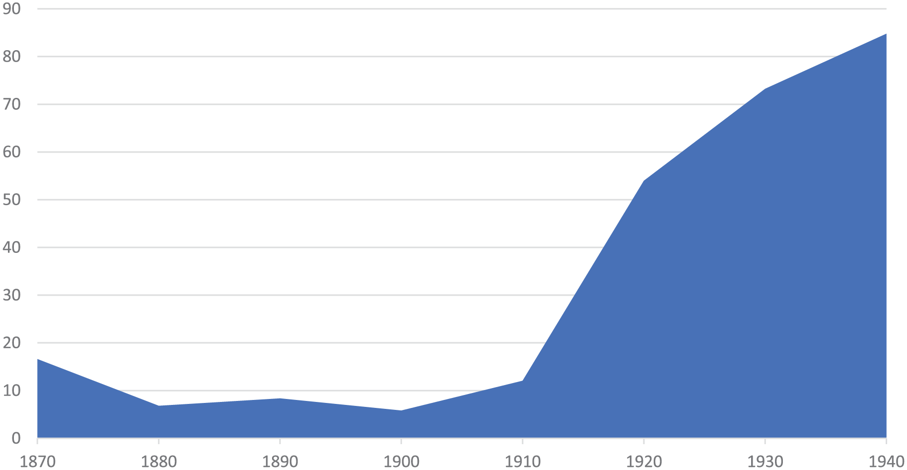
Percentage of school districts in the San Francisco Bay Area raising a district property tax, 1870–1940
Figures 2 and 3 visualize this information on a map of San Mateo and Santa Clara counties in 1890 and 1920. Only those districts shaded red raised money from district taxes to fund schools. Note how the various sizes of the districts might shape one’s perception of these data and how, at the time that these boundaries were recorded, they were not consistently being used to regulate school admissions.

School districts raising a local property tax in Marin, Napa, San Mateo, and Santa Clara counties: 1890

School districts raising a local property tax in Marin, Napa, San Mateo, and Santa Clara counties: 1920
This relationship between funding and districting policies raises a series of questions for policy researchers focused on the present. While researchers investigating school segregation often examine district boundaries, school finance scholars rarely consider how boundary manipulation through district succession and consolidation affect funding. To what extent does the degree of a state’s reliance on local financing influence the way that local communities treat their school district boundaries? To what extent do boundary changes creating uneven tax bases relate to racial segregation, and to what extent should this be acceptable practice from a legal, policy, and moral perspective? Answering these questions will help policy scholars better understand not only the spatial dimensions of school funding disparities but also the broader relationship between funding and segregation. This relationship is particularly important since researchers often argue that expanding access to school funding is one mechanism through which desegregation might increase educational opportunity (Reardon & Owens, 2014). The interplay among funding, segregation, and district boundaries is poorly understood, a point that emerges by attending to the broader historical context of spatial data.
Refining the Quantitative Geospatial Techniques Applied by Researchers
Attending to the historical context of spatial data can raise new research questions while bringing into view the importance of critical approaches to geospatial research. Incorporating a longer temporal perspective into spatial analysis can also help researchers refine the specific quantitative geospatial techniques leveraged to study contemporary policies.
Geospatial statistical methods, such as other forms of quantitative analysis, provide effective tools for applying mathematical models to study spatial relationships. As Magnus and Morgan (1999) point out with applied statistics more broadly, however, these methods on their own do not provide the theory and specific knowledge that allows researchers to generate the most impactful questions and select the best models. Here, historically contextualized spatial data can be indispensable for geospatial researchers using quantitative techniques, not only providing background knowledge that will help researchers identify appropriate models, but also helping researchers develop new measurement techniques that better capture the relationships that they aim to study.
Recent efforts to understand the relationship between school district boundaries and school segregation provide a clear example of how historicizing spatial data can support the quantitative techniques employed by geospatial education policy researchers. As more researchers use geospatial methods enabled by GIS software to study school district boundaries, some have started to investigate the extent to which the shape of attendance boundaries is associated with school segregation. In some of this work, researchers found that irregularly shaped attendance zones exacerbate racial segregation (Richards, 2014, 2017; Richards & Stroub, 2015). Other scholars examined the same geospatial data sets and found that irregularly shaped boundaries alleviate racial and income segregation in schools (Saporito, 2017; Saporito & Van Riper, 2016).
The “irregularity” of a shape is determined by comparing a given shape with some ideal shape that is not considered irregular or bizarre. The statistics enabling these comparisons are called compactness measures (Chambers & Miller, 2010). Mathematically, these measures are expressed as ratios comparing the geometric characteristics of a given shape with the characteristics of some ideal shape. Drawing on efforts to assess the irregularity of legislative districts to identify gerrymandering, Richards and Stroub (2015) used four compactness measures to assess the shape of school districts: the Polsby-Popper index, the Schwartzberg index, the convex hull index, and the Reock index. The Polsby-Popper index compares a given shape with a circle. It does this by comparing the area of a given shape with the area of a circle with a circumference that equals the original shape’s perimeter. The Schwartzberg index also compares a given shape with a circle. It does this by comparing the perimeter of a given shape to the circumference of a circle with an area that equals the original shape’s area. The Reock index also compares a shape with a circular shape. The index compares the area of a shape with the area of the smallest circle that can be drawn to enclose the entire shape (known as the minimum bounding circle). The smallest convex polygon that can be drawn around an attendance zone (a shape called the convex hull) represents the ideal compact shape assessed by the convex hull index (Young, 1988). The index compares the area of a given shape with the area of the smallest possible convex polygon that can enclose that shape. To clarify these four measures, Figure 4 displays unified school districts in 2016 with the highest and lowest index scores on each measure.

Examples of unified school districts with the highest and lowest compactness scores: 2016
Disagreement over the impact of attendance zone shape on segregation stems from differences in the way that scholars define “irregularity.” Richards and Stroub (2015)—using the Polsby-Popper index, the Schwartzberg index, the convex hull index, and the Reock index—concluded that “attendance zone boundaries are highly gerrymandered” (p. 26). In a different study, Richards (2014) compared the level of segregation created by actual attendance zones with the level expected in “natural attendance boundaries” represented by Voronoi polygons—shapes that divide space around a focal point, such as a school, in a way that “all areas within a given focal point’s polygon are closer to that focal point than to any other focal point” (p. 1127). Comparing these counterfactual boundaries with actual attendance boundaries, Richards concluded that “the gerrymandering of attendance zones generally exacerbates segregation” (p. 1119). Scholars who found that irregularly shaped boundaries alleviate racial and income segregation in schools make different assumptions about what an ideal compact shape looks like and, as a result, what measure can best assess irregularity. For example, Saporito and Van Riper (2016) combined three measures of irregularity: concavity, the Polsby-Popper index, and the convex hull index. With concavity, the ideal compact shape is any perfectly convex shape, such as a circle, rectangle, or triangle (Chambers & Miller, 2010). As is the case in the literature on legislative gerrymandering, there are multiple standardized measures of compactness developed by researchers but no universally accepted standard determining which of those methods are best (Ansolabehere & Palmer, 2016).
Research on long-term trends in school districting can provide insights into how to assess the compactness of school district and attendance zone shapes and techniques for producing new measures. For example, the history of school district boundaries in Northern California provides evidence on how boundaries were originally organized. Although early boundaries did not always determine school attendance, the original shape of districts represents a standard against which to assess the irregularity of school districts and attendance zones drawn in subsequent years. One problem with compactness measures in general is their abstract character (Ansolabehere & Palmer, 2016). An additional problem is their disconnect from the constraints imposed by higher geopolitical units and natural features. The compactness of attendance zones is shaped by the compactness of the district, county, and state within which they are located.
While researchers can control for these factors, another possible solution is to compare the compactness measures of current attendance zones and school districts with the measures assigned to shapes derived from historically contextualized studies of district boundaries. In California, school districts were originally organized in 1855 (Falk, 1968). Each civil township and incorporated city in the state were transformed into a school district by the state legislature. All future school districts and subsequent attendance zones have been created by revising these original districts. These original districts can thus serve as a reasonable, contextually appropriate benchmark for measuring compactness. Comparing four measures of compactness for current school district boundaries in Northern California with the original boundaries created in the region suggests the extent to which contemporary school district boundaries have been made irregular over time.
Along four measures of irregularity, current school districts in these counties (n = 50) are far more irregular and less compact than the original school districts created in the 1850s (n = 37). Comparing the original districts and the current districts along the four measures reveals that irregularity increased over time: Polspy-Popper index, original districts (M = .459, SD = .151) and current districts (M = .347, SD = .127); Schwartzberg index, original districts (M = .667, SD = .111) and current districts (M = .579, SD = .109); convex hull index, original districts (M = .794, SD = .143) and current districts (M = .759, SD = .092); and Reock index, original districts (M = .586, SD = .220) and current districts (M = .398, SD = .108). With all four indices, lower scores indicate greater irregularity.
The increase in irregularity assessed by the Polsby-Popper index was statistically significant, t(85) = 3.743, p < .001. The increase in irregularity assessed by the Schwartzberg index was also statistically significant, t(85) = 3.743, p < .001. The increase in irregularity assessed by the convex hull index was not statistically significant, t(85) = 5.246, p = .164. For the change in irregularity assessed by the Reock index, the assumption of homogeneity of variances was violated, as assessed by the Levene test for equality of variances (p < .001). However, running a Welch t test reveals that the increase in irregularity between original and current districts per the Reock index was statistically significant, t(48.869) = 4.781, p < .001.
The stability in the convex hull index scores between original and contemporary school districts suggests that this measure might be less sensitive to the types of changes made to school district boundaries over time, the kind of insight made possible by examining the historical context of spatial data. Multiple historical benchmarks could also be used, depending on the particular questions that researchers hope to answer. Boundaries from the 1930s, for example, could be used to assess the manipulation of boundaries during the postwar boom in California.
Extending this analysis to other regions can provide a new, contextually relevant approach to measuring district and attendance zone irregularity nationwide. Multiple measures of compactness for original districts within a region, for example, could be combined and used to create a new index for assessing district and attendance zone geography. How does the irregularity of districts or attendance zones in states with de jure segregation before Brown v. Board or Milliken v. Bradley, for example, compare with the irregularity of districts or attendance zones in more recent years?
Historicizing Spatial Data to Deepen Our Understanding of the Causes of Current Patterns
Examining the historical context of spatial data in education policy can also contribute to our broader understanding of underlying factors shaping the geospatial patterns studied by researchers. As noted here, one limitation of standard approaches to geospatial educational research is the tendency for scholars to focus on how things are, not how they got to be that way. Historicizing spatial data can help policy scholars transcend these problems, providing perspective on how particular spatial patterns emerged in the first place.
The case of research on the manipulation of district boundaries and school segregation is again instructive. Among researchers examining connections between the shape of attendance zones and segregation on a national scale, none developed a detailed explanation for the underlying causes of the patterns that they described. The reason is not that these scholars ignored questions of causality but, rather, the geospatial techniques that they employed were not sufficient, on their own, to allow them to draw such conclusions. While recent research on attendance zone irregularity included thoughtful discussion assessing potential connections between the shape of attendance boundaries and segregation, these methods did not explain how or why attendance zones developed their irregular shapes. As Richards (2014) stated clearly, spatial analysis on its own “cannot establish the intent of gerrymandering” (p. 1150). Saporito and Van Ripper (2016), too, acknowledged this limitation, discussing how their study did not “determine the intent of local school district administrators when they delineate their zones” (p. 78). Understanding intent and political process is critical to generating knowledge with the potential to transform conditions in the future.
Attending to temporal patterns can supplement this work and help researchers develop a deeper understanding of attendance zone formation. In California, for example, contemporary school district boundaries were transformed in the decades after World War II. In turn, changes to district boundaries during this period continue to determine the shape of attendance zones that can be drawn inside individual districts. In 1945, the California state legislature created the State Commission on School Districts (SCSD). The SCSD created 53 local survey committees across the state and was charged with reorganizing school district boundaries. The commission was particularly interested in school district consolidation, a long-standing goal of education reformers across the nation (Scribner, 2016; Steffes, 2011; Tyack, 1974). The reorganization process was at times slow, but the commission managed to decrease the number of school districts in the state by 57% between 1945 and 1972 (C. H. Benjamin, 1980). The records of the state and local actors involved in reorganizing district boundaries immediately after World War II have been preserved, and they reveal a great deal about the motives and intent behind changes in district boundaries during this period.
The historic record suggests that changes to school district boundaries and the irregularity in district shapes created by those changes were designed to maintain and facilitate school segregation. The SCSD created a series of documents to guide the reorganization process in the early 1950s. In its directions to local survey committees, the SCSD was explicit about the importance of using redistricting to keep students apart, rather than bring them together. While local survey committees were instructed to consider a host of factors when planning for redistricting, one consideration occupied the work of the committees more than any other: the demographic composition of a proposed district. In the guidance provided to local survey committees, the state created a series of checklists describing the most important factors to consider when creating a new district. Prominent among those were the backgrounds of the families involved and whether the new district brought together “natural groupings” of people. As the state explained in a pamphlet for local survey committees, “a sense of community membership must be preserved in the larger area proposed” (California State Commission, 1946a). In a checklist for local committees, the SCSD instructed the local survey committees to be mindful of “natural barriers” that could influence “community inclusiveness.” These “natural barriers” were social rather than geographic. Barriers related to transportation and topography were addressed in a separate category within the checklist. In a further section of the document, survey committees were instructed to make sure that any new district included people with “many common interests.” Under no circumstances should new districts, the SCSD insisted, “include sharply contrasting centers of cultural, religious, or economic interests which would probably result in discrimination against some children” (California State Commission, 1946b). Not unlike the “neighborhood unit” concept that Highsmith and Erickson (2015) identified in relation to the policies and segregationist thought facilitating school segregation in Flint, Michigan, the concept of “natural groupings” created state direction on ways to ensure that school district boundary changes maintained and exacerbated school segregation.
Surviving historical evidence suggests that the state’s instructions were carefully followed. In their reports justifying reorganization proposals, local survey committees dedicated considerable space to determining how school district reorganization could support racial and economic segregation. The San Mateo County Local Survey Committee (1949) thought primarily about “population affinities” when considering when and where school district boundaries should be redrawn and “natural groupings” that fell along racial, ethnic, and economic lines. The Santa Clara County survey committee had similar concerns when thinking about the future of school district boundaries. The committee opened its discussion of redistricting with a detailed accounting of the impact that race and ethnicity would have on district organization. The committee celebrated the “comparative freedom Santa Clara County enjoys from any racial problems” since there were only “730 Negros in the County in 1940,” with most concentrated—thanks to a host of other state policies influencing housing—in sections of the county that could become predominately non-White districts. The one concern facing the committee, it explained, was the “rather large foreign-born population which has presented some difficult problems for certain schools in the past.” While the committee was concerned that these “Portuguese, Mexican, Italian, Slavonian, or Japanese” children might not always fit together, they argued that “there is reason to believe that the problem will soon cease to have any serious effect in the schools” since “the percentage of foreign born in the county . . . is declining with each decade” (“Report of Santa Clara County Local Survey Committee,” 1948).
When they were not encouraging redistricting committees to maintain racially homogeneous districts, state officials seemed to encourage communities to use attendance boundaries to maintain segregation within districts. Indeed, the SCSD emphasized to local survey committees the role that attendance boundaries could play in ensuring that children from different backgrounds would not attend the same school, even if it otherwise made sense to put them in the same district. When a proposal for the area around Hayward seemed poised to involve the diverse community of Russell City, state officials concentrated on the difference that attendance boundaries could make for the new district. “Unification does not mean centralization of attendance,” the commissioner promised. “Quite to the contrary,” the official continued, “the ‘neighborhood’ feelings for the ‘neighborhood’ school should remain as strong under unification as at present” (Alameda-Contra Costa Counties Local Survey Committee, ca. 1949). The most studied and discussed redistricting areas involved the small number of places where African Americans were permitted to rent and purchase homes during these years. For example, in studying school districting in the area around Richmond, the local SCSD committee treated the organization of schooling in the city as a “situation deserving special consideration,” with the “situation” being the explosion of Richmond’s African American population from 270 to 14,000 between 1940 and 1945 (Alameda-Contra Costa Counties Local Survey Committee, ca. 1948; Rothstein, 2017). Since pockets of the city remained exclusively and intentionally White through a dense network of public policies, the SCSD used attendance boundaries within the district to ensure that individual schools would become racially segregated. By the 1950s, 22% of the students attending Richmond elementary schools were African American. Six of the elementary schools in the district, however, were almost completely segregated, with student populations that were >95% African American (Rothstein, 2017).
District reorganization appeared to support segregation to such an extent that state officials justified the practice and civil rights activists critiqued it. In a discussion about ways to reorganize school district boundaries involving children from diverse backgrounds, for example, one school official worried about how a proposal would “throw approximately 150 Anglo-Saxon children” into a school “entirely composed of children of Mexican extraction.” Changes like these, the official warned, would create “undesirable emotional problems on both sides” (“School Redistricting Proposal,” 1946). The tendency of education officials to “maintain separate schools by the simple device of adjusting boundary lines” under these pretenses was so widespread that a writer for the Los Angeles Sentinel cited the practice as proof that Jim Crow persisted in California (“Jim Crow Is Dying,” 1948). By 1952, the regional director of the NAACP’s West Coast branch lamented the way that “gerrymandered district lines” managed to “extend the pattern of segregation” (quoted in Brilliant, 2010, p. 234).
Any examination of boundary irregularity in California today must contend with the changes implemented during this period. Contemporary district shapes and the attendance zones drawn within them are dependent on earlier configurations. In turn, surviving historical records suggest that these configurations were deliberately manipulated to maintain segregated schooling in postwar California. Understanding the intents and motives behind the current shape of attendance zones in California then requires a significantly longer view than what a single static map can provide on its own.
Studies that historicize spatial patterns such as boundary irregularity in California can help researchers better understand the development of contemporary spatial patterns in other ways as well. The data that this research generates, for example, can allow researchers to assess how different policy shifts have affected irregularity in district and attendance zone shapes. Digitized and georeferenced district attendance zone boundary files overlaid with demographic census data could allow education policy researchers to determine how shifting jurisprudence on segregation and other policy changes have influenced the boundaries and residential patterns. How often and under what policy circumstances have changes to attendance zone and district boundaries shaped school segregation? In contrast, how often and under what circumstances have shifting residential patterns, not boundary changes, driven patterns in school segregation? Education policy research that considers the spatial and temporal context of contemporary patterns can allow scholars to answer these kinds of questions.
Conclusion: The Promise of Interdisciplinary Approaches and the Challenges of Spatial History
In recent years, geospatial techniques and methods have enhanced scholarship on education policy topics such as school choice and school district boundaries. However, Yoon and Lubienski (2018) worried that much of this work focused on the visualization of quantitative data. Gregory (2008) perhaps put it best, lamenting how this use of the software turns GIS into a program that does little more than create “bad graphs” (p. 123). A broader temporal frame can push researchers beyond this use of GIS software while enhancing the spatial analyses that they conduct. Attending to the historical context of spatial data can (1) help researchers generate new questions while developing a critical perspective on the data contained in maps, (2) provide indispensable information that can improve the geospatial measurement techniques that we use, and (3) deepen our understanding of how geography and policy have interacted over time to shape contemporary patterns in the distribution of educational opportunity. Education policy scholars do not need to complete this work on their own. Historians of education have been particularly adept at using historicized spatial data to deepen our understanding of how educational opportunity was organized in the past. K. Benjamin (2012), Dougherty (2012), Erickson (2012, 2016a, 2016b, Kitzmiller (2012), and Rury and Akaba (2014) all used GIS to generate new insights about the spatial dimensions of educational inequality in the 20th century. Scholars such as Siegel-Hawley (2016) engaged with this work to support their investigations of contemporary policies. Through more engagement with historical work and policy-focused collaboration with the historians producing it, researchers can reap the benefits of considering time and space simultaneously.
There are also clear challenges to integrating space and time in studies of education policy. The disciplinary divide between historians of education and education policy scholars can be, at times, wide (Vinovskis, 2015). Education policy scholars have not given as much attention to history as they did in the past (Wong & Rothman, 2009). Historians of education, for their part, often produce work in isolation. In an effort to understand and interpret the past on its own terms, they tend to avoid research with an explicit focus on the present. As Fraser (2015) pointed out, too many educational historians seek an audience for their work among historians across the university, instead of their colleagues across the hall.
At the same time, the nature of geospatial research offers new opportunities for transcending these challenges. Digital projects by historians can provide data and opportunities for collaboration. These “spatial history” projects often involve the time-consuming digitization of large volumes of historical data for the explicit purposes of beginning, rather than ending, the research process (White, 2010). One of the investigators of the project “Digital Harlem” quotes Thomas (2015) to define a common purpose of spatial history projects: “to open up new modes of inquiry and/or discovery” (quoted in Robertson, 2016, p. 157). This approach to spatial analysis creates new opportunities for collaboration.
By working together, policy analysts and historians can produce better geospatial work on the past and the present. Research on long-term geospatial patterns in segregation, school funding, and the distribution of economic opportunity are meaningful places for this work to start. What happens when historians and policy scholars work together to place spatial trends in a broader temporal frame? What new measures, patterns, or questions might emerge? Only by better understanding how time, space, and policy interact to shape educational opportunity can we develop a deep understanding of contemporary spatial issues in education and viable possibilities for reform in the future.