Sage Journals: Discover world-class research

Abstract

The ventriloquism aftereffect (VAE), observed as a shift in the perceived locations of sounds after audio-visual stimulation, requires reference frame (RF) alignment since hearing and vision encode space in different RFs (head-centered vs. eye-centered). Previous experimental studies reported inconsistent results, observing either a mixture of head-centered and eye-centered frames, or a predominantly head-centered frame. Here, a computational model is introduced, examining the neural mechanisms underlying these effects. The basic model version assumes that the auditory spatial map is head-centered and the visual signals are converted to head-centered frame prior to inducing the adaptation. Two mechanisms are considered as extended model versions to describe the mixed-frame experimental data: (1) additional presence of visual signals in eye-centered frame and (2) eye-gaze direction-dependent attenuation in VAE when eyes shift away from the training fixation. Simulation results show that the mixed-frame results are mainly due to the second mechanism, suggesting that the RF of VAE is mainly head-centered. Additionally, a mechanism is proposed to explain a new ventriloquism-aftereffect-like phenomenon in which adaptation is induced by aligned audio-visual signals when saccades are used for responding to auditory targets. A version of the model extended to consider such response-method-related biases accurately predicts the new phenomenon. When attempting to model all the experimentally observed phenomena simultaneously, the model predictions are qualitatively similar but less accurate, suggesting that the proposed neural mechanisms interact in a more complex way than assumed in the model.

Keywords

reference frame ventriloquism aftereffect model

Introduction

Auditory spatial perception is highly adaptive and visual signals often guide this adaptation. In the “ventriloquism aftereffect” (VAE), the perceived location of sounds presented alone is shifted after repeated presentations of spatially mismatched visual and auditory stimuli (Bertelson et al., 2006; Recanzone, 1998; Woods & Recanzone, 2004). Complex transformations of spatial representations in the brain are necessary for the visual calibration of auditory space to function correctly, as visual and auditory spatial representations differ in many important ways (Van Opstal, 2016). Here, we propose a computational model to examine the visually guided adaptation of auditory spatial representation in the VAE and the related transformations between the reference frames (RFs) of auditory and visual-spatial encoding.

We primarily examine the RF in which the VAE is induced. While visual space is initially encoded relative to the direction of eye gaze, the cues for auditory space are computed relative to the head orientation (Groh & Sparks, 1992). A means of aligning these RFs is necessary by the stage at which the visual signals guide auditory spatial adaptation. Nominally, this alignment can be achieved by either converting the visual signals to the head-centered auditory spatial representation or by transforming the auditory spatial representation into the eye-centered RF. However, other factors, like the oculomotor network driving behavior in response to the stimuli, also might play a role (Caruso et al., 2021).

Several models have been developed to describe the VAE in humans and birds. The bird models predict the VAE in the barn owls (Haessly et al., 1995; Oess et al., 2019) which cannot move their eyes and therefore their auditory and visual RFs are aligned. The existing human models mainly focus on spatial and temporal aspects of the VAE (Bosen et al., 2018; Shinn-Cunningham et al., 2005; Watson et al., 2019), not considering the different RFs. There are models of the audio-visual RF alignment for audio-visual integration (Odegaard et al., 2019; Razavi et al., 2007) and multi-sensory integration (Pouget et al., 2002) when the auditory and visual stimuli are presented simultaneously. These models apply to the ventriloquism effect which is driven by different mechanisms than the adaptation and transformations underlying the VAE (Park & Kayser, 2019, 2021).

Our experimental studies examining RF of VAE in humans and monkeys provided inconsistent results (described in detail in the following section). A mixture of eye-centered and head-centered RFs was identified for recalibration locally induced in the central region of the audio-visual field (Kopco et al., 2009) while the head-centered RF dominated when VAE was induced in the audio-visual periphery (Kopco et al., 2019). Additionally, the only other available study, in which the VAE was induced over a wide spatial area including the central region, also concluded that the RF is mixed (Watson et al., 2021). These results imply that the RF used in the VAE is dependent on the region in which the VAE is induced, possibly due to a non-homogeneity in the auditory spatial representation (Groh, 2014; Grothe et al., 2010) or due to asymmetries in the VAE generalization (Bertelson et al., 2006; Bruns & Roder, 2019). The current modeling primarily aims at identifying the neural mechanisms that underlie the mixed RF observed in the Kopco et al. (2009) and the Watson et al. (2021) studies, by implementing two specific mechanisms by which eye-centered visual signals might influence the RF of VAE, while assuming that these mechanisms act uniformly across the audio-visual field.

A secondary goal of the current modeling is to propose a mechanism to describe a new adaptive phenomenon observed in the ventriloquism study of Kopco et al. (2019) (again, described in detail in the following section). In that study, adaptation was unexpectedly induced by spatially aligned audio-visual stimuli, while no such adaptation was observed in Kopco et al. (2009).

Here, we first summarize the experimental results from Kopco et al. (2009, 2019) to explain the modeled phenomena. Then, the model is introduced and evaluated on different subsets of the Kopco et al. (2009, 2019) data. Finally, the Appendix illustrates how the model can be applied on other data by comparing the predictions of the best model fit based on the Kopco et al. data to the results of Watson et al. (2021).

Summary of Kopco et al.

The studies of Kopco et al. (2009) and (2019) induced the VAE locally in, respectively, the central or peripheral subregion of audiovisual space (Figure 1A, top). They used one initial eye fixation position on training trials and presented the discrepant audiovisual stimuli from the restricted spatial range. As the aftereffect was spatially specific, weakening outside the trained region, they could test the RF of the recalibration by shifting fixation on probe trials. Specifically, on interleaved auditory-only probe trials, they varied the initial eye position with respect to the head (which was fixed) and presented sounds from locations spanning both the same head-centered locations and the same eye-centered locations as on the training trials (see Figure 1A, bottom). The predictions of results obtained using this paradigm for central training region are illustrated in the left-hand panels of Figure 1B. If visually induced spatial plasticity occurs in a brain area using a head-centered RF, then VAE biases in perceived sound location will occur only for sounds at the same head-centered locations (in Figure 1B, blue dash-dotted line matches the red dash-dotted line). Conversely, if plasticity occurs in an eye-centered RF, then visually induced biases will occur only for sounds at the same eye-centered locations (dash-dotted cyan line is shifted to the left of the red line, staying aligned with the FP). A third possibility is that the neural mechanism involves an intermediate mixture of both RFs (a “hybrid” frame). The predicted outcomes for head- and eye-centered RFs are displayed in the bottom-left panel of Figure 1B which summarizes the potential effect as the difference between the induced bias on trials involving the training fixation and the induced bias on trials involving the non-training FP.

Figure 1.

Experimental design and results from Kopco et al. (2009, 2019). (A) Experimental design: nine loudspeakers were evenly distributed at azimuths from −30° to 30°. Two FPs were located 10° below the loudspeakers at ±11.75° from the center. On training trials, audio-visual stimuli were presented either from the central region (auditory-component at −7.5, 0 or +7.5°; Kopco et al., 2009) or peripheral region (auditory-component at 15, 22.5, or +30°; Kopco et al., 2019), while the subject fixated the training FP. The audio-visual (AV) stimuli consisted of a sound paired with an LED offset by −5°, 0°, or +5° (offset direction fixed within a session). On probe trials, the sound was presented from any of the loudspeakers while the eyes fixated one of the FPs. (B) Predicted (left-hand column) and observed (right-hand column) results for AV-misaligned training. Dash-dotted lines represent the predictions in the two RFs. Solid and dashed lines show measured across-subject mean biases in AV (green) and A-only trials (red and blue lines for respective FPs), corresponding, respectively, to the ventriloquism effect and aftereffect combined across the runs with AV-misaligned stimuli. Data from runs using V component shifted to the right and to the left are combined as no significant effect of shift direction was observed, and always plotted as if shift to the right was induced. Black lines show the differences between the respective red and blue lines, that is, differences between the biases found for the two FPs. (C) AV-aligned results: green, red, blue, and black lines as in the AV-misaligned results. Note: Error bars have been omitted for clarity. N = 7 in both experiments. All horizontal axes are plotted in head-centered RF.

The right-hand column of Figure 1B shows the experimental results from the AV-misaligned conditions (re. AV-aligned), averaged across data from runs with AV discrepancy causing a leftward and rightward VAE bias, as the difference between the two directions was not significant (note that this value is equal to the difference between the biases induced by the rightward vs. leftward shifts divided by 2). The responses to AV stimuli were always very near the visual components of the AV stimuli, in both the central and peripheral experiments (green dashed and solid lines in Figure 1B), as well as in the AV-aligned baseline (green lines in Figure 1C). The displaced V component in the AV-misaligned conditions induced a local VAE when measured with the eyes fixating the training FP (the red solid and dashed lines in Figure 1B show that maximum ventriloquism was always induced in the trained subregion of the auditory space, consistent with our predictions). The critical manipulation of these experiments was that half of the probe trials were performed with eyes fixating on a new, non-training FP (blue “+” symbol), shifted away from the training FP (red “+” symbol). The experimental data showed that, in the central experiment, moving the fixation resulted in a smaller VAE with the peak moving in the direction of eye gaze (blue vs. red dashed line), while in the peripheral experiment, only a negligible effect of the eye fixation position was observed (blue vs. red solid line).

To better visualize these results, the lower panel of Figure 1B shows data expressed as the difference between responses from training versus non-training FPs from the respective upper panels, along with the expected patterns of results for the two RFs based on the training-FP data. The head-centered RF always predicts that the effect would be identical for the two FPs. Thus, all head-centered differences (brown lines) are expected at zero. The solid and dashed yellow lines show, respectively, for the peripheral and central data, the eye-centered RF expected patterns obtained by subtracting from the red lines the same red lines shifted 23.5° to the left. Finally, the black solid and dotted lines show the actual differences between the respective red and blue data from the upper panel. For the central data, the black dashed line falls approximately in the middle between the head-centered and eye-centered predictions, showing a mixed nature of the RF of the VAE induced in this region. On the other hand, the black solid line is always near zero, showing that the RF of the VAE induced in the periphery is predominantly head-centered. The main goal of the current modeling is to examine candidate mechanisms causing these results.

While the results in Figure 1B are based on the VAE induced by AV-misaligned stimuli, Figure 1C shows the baseline data obtained in runs with auditory and visual stimuli aligned. In the central-training experiment, the responses from the two FPs were similar, unbiased at the central locations and with a slight expansive bias in the periphery (both red and blue dotted lines are near zero in the center, negative in the left-hand portion and positive in the right-hand portion of the graph). On the other hand, in the peripheral-training experiment the responses for the targets at −10 to +15° differed between the two fixations, such that the non-training FP responses fell well below the training-FP responses (compare the red and blue solid lines). Thus, the peripheral AV-aligned stimuli induced a fixation-dependent adaptation in the auditory-only responses in the central region, a VAE-like adaptation phenomenon that has not been previously reported. The black dashed and solid lines in Figure 1C, showing the difference between the corresponding red and blue data from the upper panel, highlight the FP-dependence of the peripheral data in contrast to the FP-independence in the central data. The secondary goal of the current modeling is to propose a mechanism to explain this result.

Model Description

Overview

Figure 2A shows the structure of the model. The model predicts the VAE as a function of the A-only probe azimuth and the FP location (the “response bias” vs. “probe stimulus and FP” blocks in Figure 2A). The main model component is the “auditory space representation” block that encodes the VAE biases induced by the visual ventriloquism signals (“ventriloquism” block) in head-centered coordinate frame (“HC” arrow). Additional model components, shown in gray, are optional and implement alternative mechanisms that are examined as candidates for influencing the observed RF of VAE results. The optional components “EC” arrow and “FP-dependent attenuation” block represent two different hypotheses about how EC signals might influence RF of VAE, while the “saccade-related bias” block represents biases induced when eye saccades are used as a response method. Panels B–E of Figure 2 illustrate the operation of each of the model components.

Figure 2.

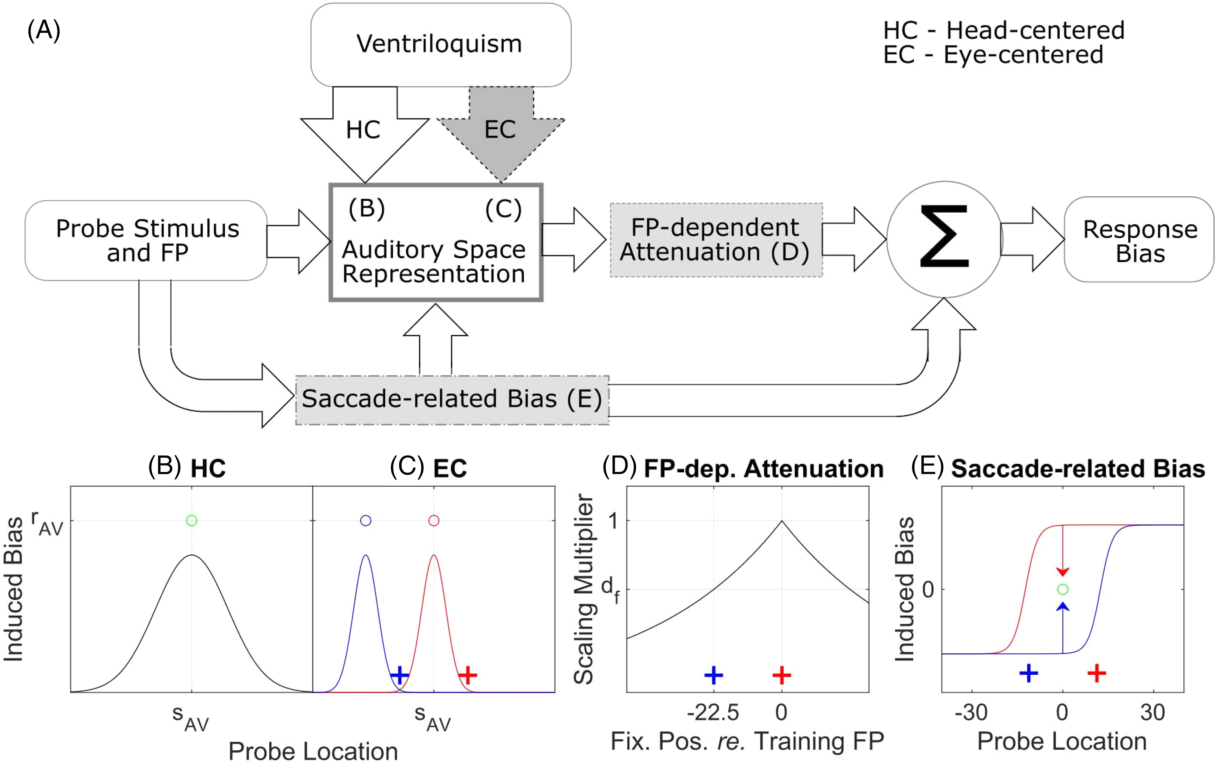
Structure of the model and illustration of its operation. (A) Block diagram of the model in which the optional model components are shown in gray. The model predicts the “response bias” for an auditory “probe location” presented while eyes fixate the location FP. The main model component is the “auditory space representation” in which biases are induced by “ventriloquism” by default in the head-centered RF (“HC” arrow). Two forms of eye-centered RF are proposed and evaluated here: (1) ventriloquism-induced biases in the eye-centered RF (“EC” arrow) and (2) “FP-dependent attenuation” of the observed VAE when eyes move away from the training FP. Finally, optional “saccade-related bias” influences the results only when saccades are used as response method. Panels B through E illustrate the operation of each of the components (see text for details).

The “auditory space representation” block assumes a continuous uniform representation of auditory space (Carlile et al., 2001) in HC frame. Its operation in the basic “HC-only” mode is illustrated in Figure 2B. The induced VAE is determined by only considering the AV stimuli used during training (3 such stimuli were used in the experiments; Figure 1A). 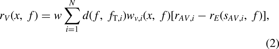For each AV stimulus, it is assumed that the induced bias (black line) is strongest at the location of the A component of the stimulus ( $s_{A V}$ ), independent of the fixation location, and that it decreases with distance from $s_{A V}$ (all in HC representation). Also, it is assumed that the overall strength of the bias is proportional to the measured ventriloquism effect at those locations ( $r_{A V}$ , represented by a green circle in Figure 2B) and the width of the neighborhood in which a given stimulus induces bias (i.e., the width of the Gaussian-shaped black line) is the same for all the AV stimuli in the HC frame. The predicted VAE is then computed simply as a sum of the effects of all the AV training stimuli. This structure of the model is consistent with the local character of VAE (Bosen et al., 2018).

The first candidate mechanism for how EC signals influence the RF of VAE assumes that the effects of ventriloquism are similar to those in the basic model but that the ventriloquism signals are in the EC RF (“EC” arrow in Figure 2A; illustrated in Figure 2C). Thus the observed effect of AV training will be constant relative to the fixation during testing (i.e., in the eye-centered coordinates). Specifically, for a training stimulus $s_{A V}$ presented while eyes fixated the “training” FP (red “+”), the VAE bias is induced at the trained location in HC frame when eyes are at the training FP during testing (red Gaussian curve) but it shifts with the eyes in HC RF when eyes move to a new non-training FP (blue “+” and the corresponding blue Gaussian). Again, the strength of the induced bias is proportional to the VE ( $r_{A V}$ represented by red and blue circles) and the width of the neighborhood is constant across the stimuli while it can be different than that for the “HC” branch (the Gaussians are narrower in panel C). This mechanism implements the hypothesized eye-centered RF as shown by cyan line in Figure 1B (Kopco et al., 2009).

The second candidate mechanism (“FP-dependent attenuation” block) assumes that the adaptation of spatial representation induced by ventriloquism is head-centered, but that the effect is multiplicatively attenuated when the eyes shift to a new FP away from the training FP (in Figure 2D, the black line has a maximum at the red training FP and decreases when eyes shift away from it, e.g., to the non-training blue FP). The attenuation is assumed to be proportional to the distance between the training and new FPs. This mechanism is motivated by the central training data in Figure 1B which shows more of an attenuation than a shift (compare red dashed vs. blue dashed data) and it might be related to FP-dependent biases observed in sound localization (Lewald & Ehrenstein, 1998; Razavi et al., 2007). Since this attenuation is dependent on the fixation location, it is also in the eye-centered RF.

Finally, the “saccade-related bias” block is an optional component that characterizes biases observed when saccades to the auditory targets are used as the response method. With it, the model proposes a mechanism that can explain the new adaptation effect observed in the no-shift peripheral-training condition (blue and red solid lines in Figure 1C). The mechanism assumes that there are a priori biases in saccade responses to auditory-only stimuli that get “corrected” by ventriloquism when aligned AV stimuli are presented on interleaved AV trials. The a priori biases are assumed to be a mixture of eye-referenced and head-referenced such that they result in hypermetric (overestimating) saccades for most stimuli except for stimuli near the median plane where they cause hypometric saccades (in Figure 2E, the red line represents this bias for the red FP, and the mirror-symmetric blue line for the blue FP). The effect of ventriloquism for aligned AV stimulus (presented, e.g., at 0°; green circle in Figure 2E) is to “correct” these a priori biases by shifting the responses toward the AV targets (arrows). The characterization of the a priori biases by sigmoidal functions (red and blue lines) was mainly chosen to be consistent with the experimental AV-aligned results from the central and peripheral experiments of Kopco et al. (red and blue lines at the non-training locations in Figure 1C). There are very few studies examining saccades to auditory targets, and their results are contradictory. This sigmoidal model is generally consistent with the results of Gabriel et al. (2010), which observed both underestimation and overestimation in saccade responses depending on the target location. Or, it is consistent with the contradictory result of (Yao & Peck, 1997), who only observed underestimation of saccade responses, when combined with overestimation in peripheral auditory localization estimates with a centrally fixed eyes (Razavi et al., 2007). Finally, a similar sigmoidal function was previously used to model visually induced spatial auditory adaptation (Zwiers et al., 2003). Importantly, here, this component only affects the predictions for the AV-aligned data, as it cancels out when considering the VAE defined as relative shifts in responses for AV-misaligned versus AV-aligned data (as shown in Figure 1B). Also, it can be simply ignored when modeling data that do not use the saccade response method, as illustrated in the Appendix which models the data of Watson et al. (2021).

There are four versions of the model evaluated here, differing by whether they include optional components “EC” arrow and “FP-dependent attenuation” subblock. The basic version of the model, referred to as “HC model”, does not include either of the optional components. Thus, it predicts that the ventriloquism signals influencing the spatial auditory representation are purely head-centered (the “HC” arrow in Figure 2A). In the “HEC model” version, the visual signals adapt the auditory spatial representation in both head-centered and eye-centered RFs (the optional “EC” arrow) such that the relative contribution of the HC and EC RFs can be arbitrary. Therefore, the HEC model reduces to the HC model if the weight of the EC path is set to zero, or it can produce predictions using only EC RF if the HC path weight is set to zero. Note that a purely EC-based version of the model was not considered as (1) the peripheral-experiment data are only consistent with a HC RF, so the model would clearly fail and (2) the HEC model could behave as such EC-only model by appropriately adjusting the relative weight, if that were the best fit to the data. The “dHC model” version only considers the “FP-dependent” attenuation component. Finally, the “dHEC model” incorporates both optional components and thus it assumes that both EC-referenced mechanisms described in the HEC and dHC models contribute to performance.

To generate the predictions, the model only uses information about the training AV stimulus locations and the average measured AV response biases for those locations. Thus, the model does not require input information about the direction of audio-visual stimulus displacement during training (whether the visual stimuli were shifted to the left, right, or aligned with the auditory stimuli). Instead, it only uses the information about where the training occurred and what the resulting ventriloquism effect was, and it assumes that there is a direct relation between the observed ventriloquism effect and aftereffect. Supporting this assumption, a comparison of the VE and VAE data at the trained locations (corresponding green and red lines in Figure 1B) shows that the VAE is approximately a half of VE at these locations in the experimental data. This allows the model to be applied to any VAE data in which the FP locations, A-component locations and AV disparities are manipulated during training. Additionally, the model can also be used to predict results of experiments for which VE values were not measured, for example, assuming that the ventriloquism capture is nearly complete, as illustrated in the Appendix simulation.

Detailed Specification

The following model specification applies to the most general dHEC model version, with the differences applying to the reduced versions described as needed (all variables in the model use the head-center representation and are in the units of degrees, unless specified otherwise).

Equation 1 describes the predicted bias in responses $\hat{r}$ to a given auditory stimulus at location s and for eyes fixating the location f as a ventriloquism-induced adaptation in auditory spatial representation $r_{V}$ combined with the optional saccade-related bias $r_{E}$ :

\hat{r} (s, f) = r_{V} (s, f) + r_{E} (s, f) .

(1)

The ventriloquism-induced adaptation is defined as:

r_{V} (x, f) = w \sum_{i = 1}^{N} d (f, f_{T, i}) w_{v, i} (x, f) [r_{A V, i} - r_{E} (s_{A V, i}, f)],

(2)

where

w \in [0, \infty]

is a free scaling parameter specifying the relative weight of the ventriloquism adaptation, d is the FP-dependent attenuation of the aftereffect in the dHC and dHEC models (Eq. 8), N is the number of combinations of training locations and FPs (in the current experiments,

N = 3

for 3 locations and 1 training fixation). For the

i

-th combination, there is a training FP

f_{T, i}

, training location azimuth

s_{A V, i}

, and the AV response bias

r_{A V, i}

obtained from the experimental data (e.g., the green data in Figure 1). The differences

r_{A V, i} - r_{E} (s_{A V, i}, f)

represent the disparity between the AV response biases and the saccade-related bias at the training locations (note that the

r_{E}

value only affects the AV-aligned data in the current simulations).

w_{v, i} (x)

is the strength with which the disparity at the

i

-th (training location × FP) combination adapts the spatial representation at the location x. In the HEC and dHEC models, this value is a weighted sum of the adaptation strengths in head-centered and eye-centered RFs, defined as:

w_{v, i} (x, f) = (1 - w_{E}) w_{v H, i} (x) + w_{E} w_{v E, i} (x, f),

(3)

where

w_{E} \in [0, 1]

is a parameter determining the relative weight of the EC-referenced contribution

w_{v H, i}

versus the HC-referenced contribution

w_{v E, i}

(in the HC and dHC models,

w_{E} = 0

). Weights

w_{v H, i}

(Eq. 4) and

w_{v E, i}

(Eq. 5) use normalized Gaussian functions centered at the training locations as a measure of the influence of

i

-th training location on target at location x, differing only in that the later uses the EC frame (all values are relative to the FP):

w_{v H, i} (x) = G (x, s_{A V, i}, σ_{H}, s_{A V}),

(4)

w_{v E, i} (x, f, f_{T, i}) = G (x - f, s_{A V, i} - f_{T, i}, σ_{E}, s_{A V} - f_{T}) .

(5)

In Eqs. (4) and (5), the bold typeface represents vectors of the length N. The normalized Gaussian dependence is defined by using normal probability density function

φ with a mean of μ

and standard deviation of

σ

G (x, μ, σ, S) = \frac{φ (\frac{x - μ}{σ})}{\sum_{i = 1}^{N} φ (\frac{S_{i} - \bar{S}}{σ})} .

(6)

In Eqs. (4) and (5), the parameters

σ_{H}

and

σ_{E}

represent the width of the influence of the ventriloquism at individual training locations, respectively, for the two RFs.

w_{v H, i}

(Eq. 4) is always centered on the

i

-th training location in the HC RF, whereas

w_{v E, i}

(Eq. 5) is centered on the

i

-th training location in the EC RF.

f_{T, i}

is the training fixation location (when

f = f_{T}

, the two RFs are aligned). Finally, the Gaussian functions are normalized (Eq. 6) such that the maximum

w_{v H, i}

w_{v E, i}

after summing across the (training FP×location) combinations equals 1.

The FP-dependent attenuation of the aftereffect is defined as

d (f, f_{T}) = d_{f}^{| f - f_{T} | / K},

(7)

which for

d_{f} < 1

is a decreasing function of the separation between

f_{T}

and f such that when the current fixation f is at the training FP

f_{T}

d = 1

, and when they are separated by K (which in the current study equal to the separation between the training and non-training FP locations),

d = d_{f}

. Note that the exact form of this dependence cannot be evaluated for the current data as only one training and one non-training fixation were evaluated.

The saccade-related bias at a specific location x for eyes fixating the location f is modeled as a sigmoidal function

r_{E} (x, f) = h (\frac{2}{1 + \exp (- k (x + c f))} - 1),

(8)

where the free parameters

h, k,

and c determine, respectively, the height, the slope, and the zero-crossing location (which equals

- c f

) of the sigmoid representing the hypometric and hypermetric biases in the saccades to auditory targets. This component, which was specifically proposed to explain the newly observed adaptation induced by the AV-aligned stimuli, can be omitted for experiments in which responses other than saccades were used. And, even in the current study, it only influences the AV-aligned predictions as it cancels out when considering the relative effect of a misaligned-AV training versus the aligned-AV training, as used here to evaluate the RF of VAE.

Simulation Methods

Stimuli

The complete data set used in the simulations consists of the AV-aligned and AV-misaligned data for the central and peripheral training regions shown in Figure 1B–C. Note that the AV-misaligned data were obtained from data with V-component shifted to the right and to the left in the original data of Kopco et al. (2009, 2019) by collapsing them across the shift direction, as no significant difference between the directions was observed. Also, the data were collapsed across the runs with training FP on the left and right, and they are always shown with the training FP on the right, the non-training FP on the left, and with the V-component shifted to the right (as in Figure 1). The training FP and non-training FP data, as well as their difference were used (blue, red, and black lines in Figure 1). Thus, the resulting complete data set contained 108 A-only across-subject mean and standard deviation stimulus-response data points ([9 azimuths] × [2 FPs + FP difference] × [2 AV conditions] × [2 training regions]); the corresponding AV training stimuli (green lines in Figure 2) were used as model parameters. In different simulations, subsets of these data were used, as described below.

Including the difference data in the current simulations was critical as that measure was the most sensitive for distinguishing between the contributions of the different RFs (as shown in the simulation results below). However, when the model is applied to other data in which it is not the difference that indicates the RF, then the difference values can be omitted (as illustrated in the Appendix).

Model Fitting and Evaluation

Four simulations were performed, each on a different subset of the data set: central simulation using central AV-misaligned data (dashed lines in the Figure 1B), peripheral simulation using peripheral AV-misaligned data (solid lines in the Figure 1B), no-shift simulation using just the AV-aligned data from both central and peripheral experiments (dashed and solid lines in the Figure 1C), and all data simulation using all data points.

Each simulation (except one) was performed by fitting the four models to the corresponding subset of the data using a two-step procedure. First, a systematic search through the parameter space was performed, using all combinations of 10 values for each parameter, listed in Table 1. Second, the best 100 parameter combinations in terms of weighted MSE were used as starting positions for non-linear iterative least-squares fitting procedure (Matlab function lsqnonlin) which, again, minimized the weighted MSE. The parameter values for the best of these fits were chosen as the optimal values listed in Table 2 and used in the result figures.

Table 1.

Range and increments of free parameters used in systematic search through the parameter space during model simulations.

Parameter	Range		Increments
Parameter	min	max	Increments
$h, w$	0	2	linear
$k$	0.01	20	quadratic
$c$	0	1.5	quadratic
$w_{E}$	0	1	linear
$σ_{H}$ ,σ_E	1	20	linear
d_f	0	1	linear

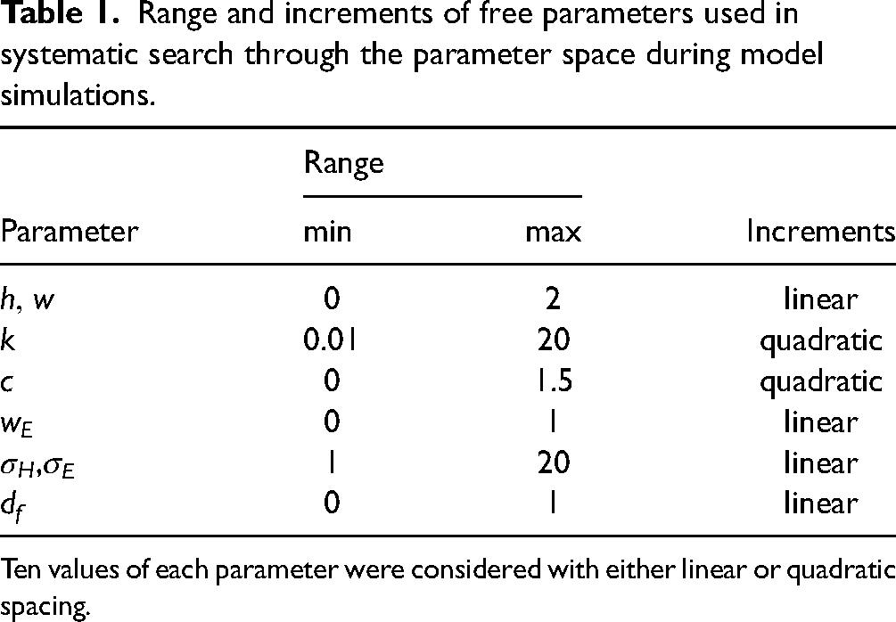
Ten values of each parameter were considered with either linear or quadratic spacing.

Table 2.

Fitted model parameters and model performance for each simulation.

Data set	Model	AICc	ΔAIC	MSE	h	k	c	w	$w_{E}$	$σ_{H}$	$σ_{E}$	$d_{f}$
Central AV-misaligned (Figure 3A)	HC	142.3	17.4	7.08	-	-	-	0.37	-	20.73	-	-
	HEC	137.7	12.7	4.48	-	-	-	0.46	0.31	21.43	5.36	-
	dHC	125.3	0.4	3.33	-	-	-	0.49	-	17.10	-	0.66
	dHEC	124.9	-	2.43	-	-	-	0.49	0.19	20.13	2.79	0.72
Peripheral AV-misaligned (Figure 3B)	HC	107.6	-	1.96	-	-	-	0.53	-	12.29	-	-
	HEC	112.8	5.2	1.84	-	-	-	0.54	0.05	12.02	4.50	-
	dHC	111.0	3.3	1.96	-	-	-	0.53	-	12.29	-	1.00
	dHEC	116.9	9.3	1.84	-	-	-	0.54	0.05	12.02	4.50	1.00
AV-aligned (Figure 3C and D)	HC	182.2	-	1.39	1.32	0.21	0.96	1.19	-	12.18	-	-
All (Figure 4)	HC	450.6	15.3	3.44	0.74	0.48	1.11	0.46	-	14.94	-	-
	HEC	441.0	5.7	3.01	0.75	0.44	1.08	0.50	0.14	14.52	4.49	-
	dHC	439.6	4.3	3.04	0.74	0.47	1.12	0.51	-	14.44	-	0.84
	dHEC	435.3	-	2.80	0.75	0.44	1.09	0.52	0.11	14.67	3.73	0.88

AICc and MSE were calculated on the data used in each simulation.ΔAIC is the increase in AICc for a given model re. the model with the lowest AICc. The underlined model names indicate the model version with substantial evidence of better fit to the data (i.e., rounded up ΔAIC smaller than 2).

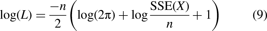
To compare the models’ performance while accounting for the number of parameters used by each model, we computed the Akaike information criterion AICc (Burnham & Anderson, 2004; Taboga, 2017) for each optimal fit, defined as:

AICc = - 2 \log (L + 2 K + 2 K \frac{K + 1}{n - K - 1},

(8)

\log (L) = \frac{- n}{2} (\log (2 π) + \log \frac{SSE (X)}{n} + 1)

(9)

where n is the number of experimental data points, K is the number of fitted parameters, and

SSE (X)

is the sum of squares of errors across the data points (i.e., differences between predictions and across-subject mean data

x_{i}

) weighted for each data point by the inverse of its across-subject standard deviation

\frac{1}{S D (x_{i})}

. In general, the model with the lower AICc is considered to be a better fit for the data. We use the rule that the model with the lower AICc is substantially better than an alternative model only if the rounded-up value ΔAIC is larger than 2.

Results

Four model evaluations were performed, each on a different subset of the data. The results of the 4 evaluations are summarized in Table 2, which shows for each simulation and model the fitted parameter values and the model's performance measured using the AICc criterion and the weighted MSE.

Central AV-Misaligned Data

Central Data simulation only fitted the central-training data from the AV-misaligned conditions (dashed lines from Figure 1B). For the mixed RF observed in these data, the simulation examined whether the eye-referenced contribution is more consistent with the eye-referenced shift in adaptation region mechanism (HEC model) or the FP-dependent attenuation mechanism (dHC model).

Figure 3A presents the results of this simulation, by showing the experimental data (now with SEM error bars) and the fitted models (lines), separately for the training FP (top panel), non-training FP (middle panel), and their difference (bottom panel). For the experimental data, the first notable observation is that the error bars on the FP-difference plots (black data in the bottom panel) are much smaller than those for the individual FPs (red and blue in top and central panels). Therefore, the critical evaluation of the current models was performed on the difference data.

Figure 3.

Model evaluation in simulations on different subsets of the data set. Model predictions (lines) and experimental data (symbols) for central AV-misaligned simulation (A), peripheral AV-misaligned simulation (B), and the central and peripheral AV-aligned simulation (shown, respectively, in the left-hand and right-hand columns of panel C). Top and middle rows: Across-subject mean biases (±SEM) and model predictions for the two FPs separately. Bottom row: Differences between the biases (±1 SEM) for the two individual FPs and corresponding differences between the model predictions from the middle and lower rows.

The top and middle panels show the data and model predictions for the two FPs separately. All the models capture the basic profile of the adaptation (note that the differences among model predictions tend to be smaller than the spread in the data). For the training FP (top panel) all the models peak at 0°, while the data peak at −7.5°. The HC model (beige) gives the worst predictions, while the dHC model (green) is closer to the data than the HEC model (magenta), in particular for the three left-most azimuths. For the non-training FP (middle panel), the HEC model captures the left-most triplet values better than the other models. However, this improved non-training FP prediction results in the non-training FP values being larger than the corresponding training-FP values (magenta line in the middle panel is above the magenta line in the top panel), causing the difference prediction (bottom panel) to have a negative undershoot, not observed in the data.

The top and middle panels also illustrate the functioning of the model for the AV-misaligned data for which only the Auditory space representation, Ventriloquism signals in HC and EC frames, and FP-dependent attenuation model components play a role. The dHC prediction (green line) in the middle panel is simply a scaled-down version of the prediction from the top panel, while the HEC prediction (magenta) has two Gaussian components that are horizontally aligned and combined in the top panel, while one of them is shifted to the left in the middle panel. The dHEC model (purple) combines these two mechanisms to obtain predictions that tend to be closest to the data.

The bottom panel offers the most direct evaluation of the models with respect to the hypothesized mechanisms. The HC model's prediction (beige) is fixed at zero, while the remaining three models fit the data better, confirming that eye-referenced signals contribute to the ventriloquism adaptation in central region (the improvement vs. HC model in terms of AICc ranges from 4.7 to 17.4). Further, the HEC model's AICc is worse by 12.3 compared to the dHC model, providing a strong evidence that the mixed RF observed behaviorally is driven by FP-dependent attenuation (dHC), not by ventriloquism signals in the EC RF (HEC). The HEC model (magenta) underestimates the central data for targets at azimuths around 0° while it predicts a negative deviation at azimuths around −20°, not observed in the data, which the dHC (green) model does not predict. Finally, the dHC and dHEC models are comparable in terms of the AICs (difference of 0.4), while the dHEC model (purple) has the lowest MSE error, indicating that the EC-referenced shift in adaptation region mechanism might have a minor additional contribution to the adaptation effect. Note that the simulation of Watson et al. (2021) data in the Appendix uses this dHEC model.

Peripheral AV-Misaligned Data

Peripheral data simulation fitted only the peripheral-training data from the AV-misaligned conditions (solid lines in Figure 1B). Table 2 shows that the HC model was indeed the best in terms of AICc and the EC-related parameters indicate a low contribution of the EC-related components in the extended models dHC/HEC ( $d_{f} = 1$ and $w_{E} = 0.05$ ). The top and middle panels of Figure 3B show that the models captured the observed ventriloquism from individual FPs well, except for the two left-most points, for which the effect appears to be negative, which the current models cannot predict as Gaussians are used to describe the local character of the VAE. The bottom panel of Figure 3B shows that, in agreement with the data, all four models produced almost identical predictions of approximately 0° difference, confirming that the RF in this experiment was largely head-centered.

Central & Peripheral AV-Aligned Data

This evaluation focused on the AV-aligned data, examining the hypothesis that the saccade-related bias combined with auditory space representation adapted in HC RF are sufficient to explain the newly observed adaptation exhibited by training-region-dependent differences in the AV-aligned data (Figure 1C). That is, it was predicted that the HC model incorporating the saccade-related bias component can accurately describe the baseline data.

Figure 3C presents the results of the HC model evaluation in a layout similar to panels A and B. However, here, both the central (left-hand column) and peripheral (right-hand column) data were fitted in one simulation. First, comparison of the error bars in the top and middle columns to the respective columns of panels A and B shows that the raw A-only responses have even much larger across-subject variability than the AV-misaligned data (which are referenced to the AV-aligned data). However, even here, computing the difference between the two FPs (bottom panel), reduces the variability dramatically. Also, the difference figure shows that the newly observed adaptation is as strong as the ventriloquism effect in this study, reaching 2–3° (compare the peaks of the black data in panel C to the red and blue peaks in panels A and B).

The HC model (beige line) captures the basic features of the AV-aligned data. Specifically, it mostly fits within the error bars for the individual FP data (red and blue), showing the FP-independent expansion of the central data (left-hand column) and the FP-dependent responses for the three central locations in the peripheral data (right-hand column). Considering the differences (bottom), the model simultaneously accounts for the null effect for the central data and the increased FP-difference in the peripheral data, suggesting that the combination of saccade-related biases and ventriloquism-mechanism correction of these biases might be underlying the newly observed adaptation. However, note that the peripheral difference data peak at 7.5° while the model prediction peaks at 0°, indicating that the interactions are more complex than those assumed here (note that without the saccade-related bias component, all these predictions would be near 0°).

All Data

In the final evaluation, the four models were fitted to all data, combining the AV-aligned and AV-misaligned data from central and peripheral experiments (solid and dotted lines from Figure 1B and C). The evaluation examined whether the model predictions, which were accurate on separate data subsets, will also be accurate when the subsets are combined, and whether the conclusions drawn on the subset simulations will generalize to the combined data. Figure 4 presents the results of this simulation using a layout similar to Figure 3. Overall, the model predictions in this simulation are less accurate than in the separate data set simulations (previous sections), mostly following the same trends as observed there. For the AV-misaligned data, the training-FP and non-training FP predictions are fairly accurate for peripheral data (top and middle row of Figure 4B), again with the exception that the current model cannot predict the negative bias at the left-most locations. On the other hand, the predictions for the central data show larger departures, especially for the 0–15° locations and non-training FP (middle panel of Figure 4A), for which the bias in data is reduced more than the models predict. Also, for the central training-FP data, the model predictions peak at 0° for all the models while the data peak is shifted to the left (top panel of Figure 4A). However, overall, the different models produce very similar predictions when considering the FPs separately, especially when compared to the individual differences in the data (across-subject variability in top and middle panels of Figure 4A–B).

Figure 4.

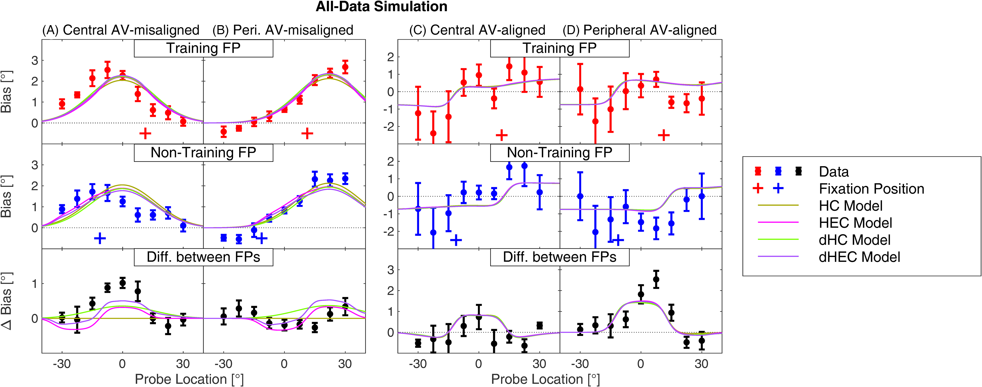
A model evaluation performed on all data combined. The layout, color scheme, and other aspects as in Figure 3.

The FP-difference plots in the bottom panels of Figure 4A–B allow us to focus on the differences between models. They show that the models tend to underestimate the FP-difference in the central AV-aligned data, in particular at azimuths near 0°, while they overestimate the FP-difference in the peripheral data, especially at azimuths 15–22.5°. This pattern of results is caused by the largely linear operation of the model, which causes that the peripheral-data and central-data predictions are approximately identical when aligned with respect to the training region (i.e., the individual lines in the right-hand panel, when shifted to the left by 23.5°, are almost identical to the lines in the left-hand panel). Then, to minimize the error for both central and peripheral data, the models’ predictions are approximately in the middle of these two data sets. However, even with this constraint, the dHC and dHEC models perform significantly better than the HC and HEC model in terms of AICc (Table 2), again supporting the conclusion that the FP-dependent attenuation mechanism is the most likely mechanism causing the mixed RF observed for the central data, while the HEC mechanism only has a small contribution.

Finally, the predictions for the AV-aligned data (Figure 4C–D) are again less accurate than when these data were considered separately (Figure 3C) and with very small differences among the models, confirming that the main mechanism allowing accurate predictions is the saccade-related bias. Focusing on the FP-difference panels (bottom row), the models do qualitatively capture that the biases are larger for the middle targets in the peripheral (panel D) than in the central (panel C) region. This less accurate prediction is caused mainly by the fact that the parameter w needs to be large in order for the combination of saccade-related bias and ventriloquism adaptation to produce accurate predictions (it is more than 1 in the AV-aligned simulation), while it is only around 0.5 in the simulations involving AV-misaligned data (this simulation, as well as the Central and Peripheral AV-misaligned simulations in Table 2).

Discussion

This study introduced a model of the RF of the VAE and evaluated it on data from three previous studies. The model considers two forms of eye-centered signals influencing the auditory space representation: ventriloquism signals in eye-centered RF and FP-dependent attenuation. The main evaluation of the model, performed on the central-training data from Kopco et al. (2009), found the FP-dependent attenuation mechanism to be the main eye-centered mechanism that caused the mixed RF reported in that study. And, this model can also correctly predict the data from Watson et al. (2021), simulated in the Appendix. This result suggests that the auditory space representation is natively head-centered, that is, that the visual ventriloquism signals are primarily converted to the HC frame before affecting the auditory spatial representation. The main contributor to the observed mixed RF is then the FP-dependent attenuation of the adaptation. While this mechanism is computationally very simple, only dependent on the relative location of the current testing FP re. training FP, it is not immediately obvious how the mechanism is implemented neurally. One possibility is that the visual representation of the training FP is adapted due to the eyes fixating mostly on that location during the training, this resulting in a stronger VAE from that location. Another option is that it is related to the saccade response method used in the current study, which would need to be adapted beyond the saccade-related biases considered here. However, given that the current modeling is also consistent with the results of Watson et al. (2021), this interpretation is not likely.

For the peripheral-training data from Kopco et al. (2019), the current modeling confirmed that the RF of VAE is only head-centered. This is consistent with the central-data results suggesting that the ventriloquism adaptation is only in the HC RF, but it is not clear why the FP-dependent attenuation is not observed here. One possible explanation is that the attenuation only affects the results when the induced adaptation causes a mixture of hypermetric and hypometric saccade adaptation (which was the case for the central training, but not for the peripheral training). Alternatively, it might be related to the character of the auditory spatial representation. For example, if that representation is not uniform as assumed here, then it might be affected differently when training is in the center versus in the periphery.

The model was also able to explain a new form of auditory space adaptation induced by AV-aligned stimuli in Kopco et al. (2019). To this end, it proposed a specific form of interaction between saccade-related bias and the ventriloquism adaptation which assumes that the VAE measured by saccades is influenced by the motor representations guiding the saccades to AV and/or auditory targets. This mechanism cannot be directly verified as currently available data are not consistent in terms of whether saccades to auditory targets are predominantly hypermetric or hypometric (Gabriel et al., 2010; Yao & Peck, 1997), while even less is known about saccades to misaligned AV targets (while those are typically assumed to have a small effect; (Caruso et al., 2021)). Additionally, eye-gaze-direction-dependent biases in sound localization have been previously observed even when saccades are not used for responding (Lewald & Ehrenstein, 1998; Razavi et al., 2007), and these likely also influence the measured saccade biases. To tease these contributions apart, future studies need to assess the RF using response methods other than saccades (Kopco et al., 2015; Lewald & Ehrenstein, 1998).

Finally, when the AV-aligned and AV-misaligned data from both studies were combined, the model predictions became less accurate, likely due to the limited linear interactions of the model components considered here. However, the model evaluation on the combined data still qualitatively supported the conclusions obtained in the separate evaluations, suggesting a dominant role of the FP-dependent attenuation. To accurately predict all the data, the model could be extended by (1) a plausible mechanism that results in FP-dependent attenuation only when the training region covers the midline (to correctly predict both the central and the peripheral AV-misaligned data) and (2) adaptive AV-condition-dependent strength of the ventriloquism component (w parameter needs to be around 0.5 for the AV-misaligned data and more than 1 for the AV-aligned data).

The current model only uses the responses on AV training trials to predict the ventriloquism adaptation, independent of the size of the audio-visual disparity or of whether the disparity results in hypometric or hypermetric saccades. And it assumes that the ratio of observed VAE to the effect is constant, in our studies at approximately 0.5 (for the AV-misaligned data). With this simple assumption the model can also be applied to predict the results of other VAE studies, even those in which the ventriloquism effect was not measured (as the ventriloquism effect is typically near complete, as illustrated here in Figure 1), and those that did not use saccades for responding (the optional saccade-related bias component of the model can be simply omitted), as illustrated in the Appendix.

The basic assumption of the model is that the VAE can be induced locally, in a Gaussian-shaped neighborhood around the auditory component of the AV stimulus (Figure 2B). With this assumption, the model fits both the central and peripheral AV-misaligned data more accurately than, for example, the triangular neighborhood of Bosen et al. (2018). However, there are two aspects of the model that can be improved. First, for the central data, the training resulted in asymmetrical adaptation that was shifted away from the training FP. A FP-dependent scaling of the adaptation could describe this asymmetry. Interestingly, note that if this asymmetry was implemented, that would make the training-FP model predictions shifted even more towards the non-training FP predictions, thus making the contribution of the HEC component even smaller than currently reported. Second, for the peripheral training, the locally induced aftereffect resulted in a small negative aftereffect in the hemifield opposite to the training hemifield. Replacement of the Gaussian by a more complex function, like a difference of Gaussians, could describe this effect (Marr & Hildreth, 1980). Also, some studies have reported stronger generalization within than across hemifields or stronger generalization on the side of the visual component versus the opposite side (e.g., Bertelson et al., 2006; Bruns & Roder, 2019). Incorporating these results could further enhance the accuracy of the current model predictions.

The neural mechanisms of the VAE and its RF are not well understood. Cortical areas involved in VAE likely include Heschl's gyrus, planum temporale, intraparietal sulcus, and inferior parietal lobule (Michalka et al., 2016; Van Der Heijden et al., 2019; Zatorre et al., 2002; Zierul et al., 2017). Multiple studies found some form of hybrid representation or mixed auditory and visual signals in several areas of the auditory pathway, including the inferior colliculus (Zwiers et al., 2004), primary auditory cortex (Werner-Reiss et al., 2003), the posterior parietal cortex (Duhamel et al., 1997; Mullette-Gillman et al., 2005, 2009), as well as in the areas responsible for planning saccades in the superior colliculus and the frontal eye fields (Schiller et al., 1979; Wallace & Stein, 1994). In the current model, the saccade-related component likely corresponds to the saccade-planning areas. The auditory space representation component likely corresponds to the primary or the higher auditory cortical areas, or the posterior parietal areas.

There is growing evidence that, in mammals, auditory space is primarily encoded based on two or more spatial channels roughly aligned with the left and right hemifields of the horizontal plane (Groh, 2014; Grothe et al., 2010; Mcalpine et al., 2001; Salminen et al., 2009; Stecker et al., 2005). Considering such an extension might improve the current model's ability to predict the central and peripheral data simultaneously. However, importantly, such opponent-processing model cannot easily model the locally induced adaptation in the current central data, as the hemispheric adaptation would always influence a whole hemifield. Thus, as a minimum, it would require a third, central channel, as proposed, for example, by Dingle et al. (2012).

While most recalibration studies examined the aftereffect on the time scales of minutes (Radeau & Bertelson, 1974, 1976; Recanzone, 1998; Woods & Recanzone, 2004), recent studies demonstrated that it can be elicited very rapidly, for example, by a single trial with audio-visual conflict (Wozny & Shams, 2011). If it is the case that the adaptive processes underlying the VAE occur on multiple time scales, as also suggested in several models of slower VAE (Bosen et al., 2018; Watson et al., 2019), then an open question is whether the RF is the same at the different scales or whether it is different. The current results are mostly applicable to the slow adaptation on the time scale of minutes, while the RF on the shorter time scales has not been previously explored (even though the Kopco et al. data might have a transitory component as well sing the training and testing trials were interleaved there). However, note that the Watson et al. (2021) data only show mixed RFs at shorter time scales of training (up to 70 s), while training with duration of 140 s resulted in no evidence of the mixed RF, largely consistent with the current conclusions of the dominant role of the head-centered RF of VAE. Future experimental and modeling studies need to address these temporal aspects of the RF of VAE.

Footnotes

Acknowledgments

The authors thank Piotr Majdak for his comments on an early version of this manuscript.

Data Availability Statement

All data and code are available on GitHub:

Declaration of Conflicting Interests

The authors declared no potential conflicts of interest with respect to the research, authorship, and/or publication of this article.

Funding

The authors disclosed receipt of the following financial support for the research, authorship, and/or publication of this article: This work was supported by the Slovak Scientific Grant Agency VEGA (Grant no. 1/0350/22) and EU Danube Region Strategy grant ASH (Grant Nos. APVV DS-FR-19-0025, WTZ MULT 07/2020, 45268RE).

ORCID iD

Norbert Kopčo

Appendix

To illustrate that the current model can be applied to data other than Kopco et al. (2009, 2019), this section evaluates the model on the data of Watson et al. (2021), to our knowledge the only other study that examined the RF of the VAE. This study used a different experimental paradigm to evaluate the RF and came with a conclusion that the RF is a mixture of eye- and head-centered frames, similar to the central-training experiment of Kopco et al. (2009).

The experimental design of Watson et al. (2021) is illustrated in Figure 5A–C, using a layout similar to Figure 1. Similar to the Kopco et al. (2009, 2019) studies, Watson et al. (2021) presented audio-visual stimuli from multiple locations while also manipulating the training FP. They used a much larger AV discrepancy (20°), did not have an AV-aligned condition, and their training and testing blocks were separate, implying a much larger time between the training and testing compared to the interleaved training and testing trials in Kopco et al. Also, they examined different time scales of adaptation (ranging from 35 to 140 s), and their conclusions of mixed RF of VAE are based on averaging across those time scales (as also used here), even though the data show a trend suggesting that at a large time scale the RF of VAE is only head-centered. In Figure 5A–C, the red “+” signs represent the training FP, the horizontal location of the green squares represents the horizontal location of the A component of the AV stimuli in the HC frame, and the vertical location represents the offset of the V component re. the A component (dotted connections link the combinations of FP and AV stimuli used in a given condition). Note that the design was symmetrical, also using the −20° discrepancy (i.e., for each [red “+” × green square] combination in Figure 5A–C, there was also a combination of the FP and AV stimulus symmetrical around 0°). In the Eye-Head-Consistent condition (Figure 5A), the FP was fixed at 0° and the AV stimuli were presented with the A-component at −50° to +30° (in 10° steps) and the V-component offset by +20°. Thus, the stimulation was consistent in both HC and EC RFs. In the Eye-Consistent condition (Figure 5B), the A-component was fixed at −20°, while the FP and V-component moved congruently from −30° to +30°. Thus, the visual signals were always at 0° in the EC RF (consistent with the A-component at −20° in the HC RF), but the AV disparity varied from trial to trial. Finally, in the Head-Consistent condition (Figure 5C), the FP and V-component moved congruently from −30° to +30°, while the A-component was always −20° to the left of the V-component. Thus, the visual signals in HC were always displaced by 20° from the A-component in the HC RF, but the visual signals in EC RF provided inconsistent information since they were always at 0°.

The performance was evaluated in a test block in which the FP was at 0° and the A-only signals were presented from the range of −30° to +30°. The bias and gain in the linear fit to the responses was estimated, and the difference between biases obtained in this fit for the −20° versus +20° AV displacement was the main indicator of the RF of VAE. This difference, shown as bars in Figure 5D, was the largest when the ventriloquism signals were consistent in both RFs (Eye-Head-Consistent condition), while it was reduced when the visual signals were consistent in only one RF (Eye-Consistent and Head-Consistent conditions), indicating that visual signals need to be consistent in both RFs to achieve maximum VAE, and thus that the RF is mixed.

Since the training region in the Watson et al. study was mostly overlapping with the central training region of Kopco et al. (2009), we selected dHEC model, the best-performing model from the central data evaluation, and generated the predictions of that model (without the saccade-related bias component) using the model parameters obtained in the simulation (Table 2). Purple lines in Figure 5A–C show the predictions of the model, exhibiting biases that decrease approximately linearly with target azimuth and have one or multiple peaks (Watson et al. do not report the corresponding data). Linear fits to these predictions were computed and the bias difference for the −20° versus +20° AV displacement was determined for each condition, shown by the purple line in Figure 5D. The results show that the dHEC model overestimated the measured bias differences mainly for the Eye-Head-Consistent condition. This difference might be caused by the differences in the experimental design. Specifically, the Watson study used a much larger AV disparity of 20° and a much larger training-to-testing delay (separate blocks vs. interleaved trials in Kopco et al.) which likely caused that the resulting aftereffect was weaker. However, most importantly, the dHEC model correctly predicts that the Eye-Consistent and Head-Consistent bias would be weaker than the Eye-Head-Consistent bias. Thus, it can be concluded that the Watson et al. (2021) results are consistent with the results of the current modeling, suggesting that the mechanism causing the apparent mixed RF of VAE is mainly the FP-dependent attenuation, not the visual signals in EC RF. However, since Watson et al. introduced the VAE broadly not locally, and the resulting adaptation was largely linear, it is difficult to use these data to distinguish between the mechanisms driving the EC contributions.

References

Bertelson

Frissen

Vroomen

De Gelder

(2006). The aftereffects of ventriloquism: Patterns of spatial generalization. Perception and Psychophysics, 68(8), 428–436. https://doi.org/10.3758/BF03193687

Bosen

A. K.

Fleming

J. T.

Allen

P. D.

O’Neil

W. E.

Paige

G. D.

(2018). Multiple time scales of the ventriloquism aftereffect. PLoS ONE, 13(8), 1–20. https://doi.org/10.1371/journal.pone.0200930

Bruns

Roder

(2019). Spatial and frequency specificity of the ventriloquism aftereffect revisited. Psychological Research, 83(7), 1400–1415. https://doi.org/10.1007/s00426-017-0965-4

Burnham

K. P.

Anderson

D. R.

(2004). Multimodel inference understanding AIC and BIC in model selection. Sociological Methods & Research, 33(2), 261–304. https://doi.org/10.1177/0049124104268644

Carlile

Hyams

Delaney

(2001). Systematic distortions of auditory space perception following prolonged exposure to broadband noise. Journal of the Acoustical Society of America, 110(1), 416–424. https://doi.org/10.1121/1.1375843

Caruso

V. C.

Pages

D. S.

Sommer

M. A.

Groh

J. M.

(2021). Compensating for a shifting world: Evolving reference frames of visual and auditory signals across three multimodal brain areas. Journal of Neurophysiology, 126(1), 82–94. https://doi.org/10.1152/jn.00385.2020

Dingle

R. N.

Hall

S. E.

Phillips

D. P.

(2012). The three-channel model of sound localization mechanisms: Interaural level differences. The Journal of the Acoustical Society of America, 131(5), 4023–4029. https://doi.org/10.1121/1.3701877

Duhamel

J.-R.

Bremmer

Benhamed

Graf

(1997). Spatial invariance of visual receptive fields in parietal cortex neurons. Nature, 389(6653), 845–848. https://doi.org/10.1038/39865

Gabriel

D. N.

Munoz

D. P.

Boehnke

S. E.

(2010). The eccentricity effect for auditory saccadic reaction times is independent of target frequency. Hearing Research, 262(1-2), 19–25. https://doi.org/10.1016/j.heares.2010.01.016

10.

Groh

J. M.

(2014). Making space: How the brain knows where things are. Harvard University Press.

11.

Groh

J. M.

Sparks

D. L.

(1992). Two models for transforming auditory signals from head-centered to eye-centered coordinates. Biological Cybernetics, 67(4), 291–302. https://doi.org/10.1007/BF02414885

12.

Grothe

Pecka

Mcalpine

(2010). Mechanisms of sound localization in mammals. Physiological Reviews, 90(3), 983–1012. https://doi.org/10.1152/physrev.00026.2009

13.

Haessly

Sirosh

Miikkulainen

(1995). A model of visually guided plasticity of the auditory spatial map in the barn owl. In Moore

JD.

& Lehman

(Eds.), Seventeenth annual meetings of the cognitive science society (pp. 154–158). Erlbaum.

14.

Kopco

Lin

I. F.

Shinn-Cunningham

B. G.

Groh

J. M.

(2009). Reference frame of the ventriloquism aftereffect. Journal of Neuroscience, 29(44), 13809–13814. https://doi.org/10.1523/JNEUROSCI.2783-09.2009

15.

Kopco

Loksa

Lin

I. F.

Groh

Shinn-Cunningham

(2019). Hemisphere-specific properties of the ventriloquism aftereffect. The Journal of the Acoustical Society of America, 146(2), EL177–EL183. https://doi.org/10.1121/1.5123176

16.

Kopco

Marcinek

Tomoriova

Hladek

(2015). Contextual plasticity, top-down, and non-auditory factors in sound localization with a distractor. Journal of the Acoustical Society of America, 137(4), EL281–EL287. https://doi.org/10.1121/1.4914999

17.

Lewald

Ehrenstein

W. H.

(1998). Auditory-visual spatial integration: A new psychophysical approach using laser pointing to acoustic targets. Journal of the Acoustical Society of America, 104(3), 1586–1597. https://doi.org/10.1121/1.424371

18.

Marr

Hildreth

(1980). Theory of edge detection. Proceedings of the Royal Society of London. Series B, Biological Sciences, 207(1167), 215–217. https://doi.org/10.1098/rspb.1980.0020

19.

Mcalpine

Jiang

Palmer

A. R.

(2001). A neural code for low-frequency sound localization in mammals. Nature Neuroscience, 4(4), 396–401. https://doi.org/10.1038/86049

20.

Michalka

S. W.

Rosen

M. L.

Kong

Shinn-Cunningham

Somers

D. C.

(2016). Auditory spatial coding flexibly recruits anterior, but not posterior, visuotopic parietal cortex. Cerebral Cortex, 26(3), 1302–1308. https://doi.org/10.1093/cercor/bhv303

21.

Mullette-Gillman

O. A.

Cohen

Y. E.

Groh

J. M.

(2005). Eye-centered, head-centered, and complex coding of visual and auditory targets in the intraparietal sulcus. Journal of Neurophysiology, 94(4), 2331–2352. https://doi.org/10.1152/jn.00021.2005

22.

Mullette-Gillman

O. A.

Cohen

Y. E.

Groh

J. M.

(2009). Motor-related signals in the intraparietal cortex encode locations in a hybrid, rather than eye-centered, reference frame. Cerebral Cortex, 19(8), 1761–1775. https://doi.org/10.1093/cercor/bhn207

23.

Odegaard

Beierholm

U. R.

Carpenter

Shams

(2019). Prior expectation of objects in space is dependent on the direction of gaze. Elsevier Cognition, 182, 220–226. https://doi.org/10.1016/j.cognition.2018.10.011

24.

Oess

Ernst

M. O.

Neumann

(2019). Computational investigation of visually guided learning of spatially aligned auditory maps in the colliculus. Proceedings of the International Symposium on Auditory and Audiological Research, 16(7), 149–156. https://doi.org/10.1101/2020.02.03.931642

25.

Park

Kayser

(2019). Shared neural underpinnings of multisensory integration and trial-by-trial perceptual recalibration in humans.. eLife, 8(e47001), 1–24. https://doi.org/10.7554/eLife.47001

26.

Park

Kayser

(2021). The neurophysiological basis of the trial-wise and cumulative ventriloquism aftereffects. The Journal of Neuroscience, 41(5), 1068–1079. https://doi.org/10.1523/JNEUROSCI.2091-20.2020

27.

Pouget

Deneve

Duhamel

J. R.

(2002). A computational perspective on the neural basis of multisensory spatial representations. Nature Reviews Neuroscience, 3(9), 741–747. https://doi.org/10.1038/nrn914

28.

Radeau

Bertelson

(1974). The after-effects of ventriloquism. Quarterly Journal of Experimental Psychology, 26(FEB), 63–71. https://doi.org/10.1080/14640747408400388

29.

Radeau

Bertelson

(1976). The effect of a textured visual field on modality dominance in a ventriloquism situation. Perception and Psychophysics, 20(4), 227–235. https://doi.org/10.3758/BF03199448

30.

Razavi

O’Neill

W. E.

Paige

G. D.

(2007). Auditory spatial perception dynamically realigns with changing eye position. Journal of Neuroscience, 27(38), 10249–10258. https://doi.org/10.1523/JNEUROSCI.0938-07.2007

31.

Recanzone

G. H.

(1998). Rapidly induced auditory plasticity: The ventriloquism aftereffect. Proceedings of the National Academy of Sciences of the United States of America, 95(3), 869–875. https://doi.org/10.1073/pnas.95.3.869

32.

Salminen

N. H.

May

P. J.

Alku

Tiitinen

(2009). A population rate code of auditory space in the human cortex. PLoS One, 4(10), 1–9. https://doi.org/10.1371/journal.pone.0007600

33.

Schiller

P. H.

True

S. D.

Conway

J. L.

(1979). Effects of frontal eye field and superior colliculus ablations on eye movements. Science, 206(4418), 590–592. https://doi.org/10.1126/science.115091

34.

Shinn-Cunningham

B. G.

Kopco

Martin

T. J.

(2005). Localizing nearby sound sources in a classroom: Binaural room impulse responses. Journal of the Acoustical Society of America, 117(5), 3100–3115. https://doi.org/10.1121/1.1872572

35.

Stecker

G. C.

Harrington

I. A.

Middlebrooks

J. C.

(2005). Location coding by opponent neural populations in the auditory cortex. PLoS Biology, 3(3), e78. https://doi.org/10.1371/journal.pbio.0030078

36.

Taboga

(2021). "Normal distribution - Maximum likelihood estimation." Lectures on probability theory and mathematical statistics. Kindle Direct Publishing, Online Appendix. Retrieved from https://www.statlect.com/fundamentals-of-statistics/normal-distribution-maximum-likelihood.

37.

Van Der Heijden

Rauschecker

J. P.

De Gelder

Formisano

(2019). Cortical mechanisms of spatial hearing. Nature Reviews Neuroscience, 20(10), 609–623. https://doi.org/10.1038/s41583-019-0206-5

38.

Van Opstal

(2016). The auditory system and human sound-localization behavior (1st ed., pp. 1–22). Elsevier.

39.

Wallace

M. T.

Stein

B. E.

(1994). Cross-modal synthesis in the midbrain depends on input from cortex. Journal of Neurophysiology, 71(1), 429–432. https://doi.org/10.1152/jn.1994.71.1.429

40.

Watson

D. M.

Akeroyd

M. A.

Roach

N. W.

Webb

B. S.

(2019). Distinct mechanisms govern recalibration to audio-visual discrepancies in remote and recent history. Scientific Reports, 9(1), 1–12. https://doi.org/10.1038/s41598-019-44984-9

41.

Watson

D. M.

Akeroyd

M. A.

Roach

N. W.

Webb

B. S.

(2021). Multiple spatial reference frames underpin perceptual recalibration to audio-visual discrepancies. PLoS One, 16(5), 1–21. https://doi.org/10.1371/journal.pone.0251827

42.

Werner-Reiss

Kelly

K. A.

Trause

A. S.

Underhill

A. M.

Groh

J. M.

(2003). Eye position affects activity in primary auditory cortex of primates. Current Biology, 13(7), 554–562. https://doi.org/10.1016/S0960-9822(03)00168-4

43.

Woods

T. M.

Recanzone

G. H.

(2004). Visually induced plasticity of auditory spatial perception in macaques. Current Biology, 14(17), 1559–1564. https://doi.org/10.1016/j.cub.2004.08.059

44.

Wozny

D. R.

Shams

(2011). Recalibration of auditory space following milliseconds of cross-modal discrepancy. Journal of Neuroscience, 31(12), 4607–4612. https://doi.org/10.1523/JNEUROSCI.6079-10.2011

45.

Yao

Peck

C. K.

(1997). Saccadic eye movements to visual and auditory targets. Experimental Brain Research, 115(1), 25–34. https://doi.org/10.1007/PL00005682

46.

Zatorre

R. J.

Bouffard

Ahad

Belin

(2002). Where is ‘where’ in the human auditory cortex? Nature Neuroscience, 5(9), 905–909. https://doi.org/10.1038/nn904

47.

Zierul

Roder

Tempelmann

Bruns

Noesselt

(2017). The role of auditory cortex in the spatial ventriloquism aftereffect. Neuroimage, 162, 257–268. https://doi.org/10.1016/j.neuroimage.2017.09.002

48.

Zwiers

M. P.

Van Opstal

A. J.

Paige

G. D.

(2003). Plasticity in human sound localization induced by compressed spatial vision. Nature Neuroscience, 6(2), 175–181. https://doi.org/10.1038/nn999

49.

Zwiers

M. P.

Versnel

Van Opstal

A. J.

(2004). Involvement of monkey inferior colliculus in spatial hearing. The Journal of Neuroscience, 24(17), 4145–4156. https://doi.org/10.1523/JNEUROSCI.0199-04.2004

Toward a Unified Theory of the Reference Frame of the Ventriloquism Aftereffect

Abstract

Keywords

Introduction

Summary of Kopco et al.

Model Description

Overview

Detailed Specification

Simulation Methods

Stimuli

Model Fitting and Evaluation

Results

Central AV-Misaligned Data

Peripheral AV-Misaligned Data

Central & Peripheral AV-Aligned Data

All Data

Discussion

Footnotes

Acknowledgments

Data Availability Statement

Declaration of Conflicting Interests

Funding

ORCID iD

Appendix

References