Sage Journals: Discover world-class research

Abstract

Speech and music both play fundamental roles in daily life. Speech is important for communication while music is important for relaxation and social interaction. Both speech and music have a large dynamic range. This does not pose problems for listeners with normal hearing. However, for hearing-impaired listeners, elevated hearing thresholds may result in low-level portions of sound being inaudible. Hearing aids with frequency-dependent amplification and amplitude compression can partly compensate for this problem. However, the gain required for low-level portions of sound to compensate for the hearing loss can be larger than the maximum stable gain of a hearing aid, leading to acoustic feedback. Feedback control is used to avoid such instability, but this can lead to artifacts, especially when the gain is only just below the maximum stable gain. We previously proposed a deep-learning method called DeepMFC for controlling feedback and reducing artifacts and showed that when the sound source was speech DeepMFC performed much better than traditional approaches. However, its performance using music as the sound source was not assessed and the way in which it led to improved performance for speech was not determined. The present paper reveals how DeepMFC addresses feedback problems and evaluates DeepMFC using speech and music as sound sources with both objective and subjective measures. DeepMFC achieved good performance for both speech and music when it was trained with matched training materials. When combined with an adaptive feedback canceller it provided over 13 dB of additional stable gain for hearing-impaired listeners.

Keywords

Feedback cancellation deep learning speech perception coloration effect howling

Introduction

Speech and music are two types of sounds that have been widely used in studies of auditory perception (Fastl & Zwicker, 2007; Darwin, 2009; Roederer, 2009; Moore, 2013). Speech provides a natural and effective means of communication while music enhances social interactions, brings pleasure, and conveys emotions. Both speech and music perception are important for hearing-impaired people, but devices such as hearing aids are designed primarily to improve speech perception, with less focus on music perception.

Both speech and music are highly non-stationary and have a large dynamic range. The level of speech ranges from about 30 dB sound pressure level (SPL) for a whisper to about 85 dB SPL for a shouted voice, the level of normal conversation being about 60 dB SPL (Zhang & Hansen, 2007; Moore et al., 2008). The level of live music can be as low as 30 dB SPL while the peak levels can reach 115–120 dB SPL, depending on the type of instruments and on whether amplification is used (Hockley et al., 2012; Chasin & Hockley, 2014; Moore, 2022). Speech and music also differ in many other ways. One is that speech often contains silent pauses, typically before and after stop consonants (Brady, 1965), while music can contain long passages without any pauses. A second is that speech can be recursively predicted, as shown by a well-known speech production model (Atal & Schroeder, 1970; Saito et al., 1970; Makhoul, 1975; Quatieri, 2006), while music usually cannot be modeled in this way. A third is that music often contains components that are stable over tens or hundreds of milliseconds, while the fundamental frequency of voiced speech usually changes rapidly over time. These different characteristics of speech and music make it difficult to develop a unified approach to signal processing in hearing aids.

It is common to use different strategies when processing speech and music for both normal-hearing (NH) and hearing-impaired listeners. Noise suppression based on time-frequency analysis is often used to reduce noise and improve speech quality for NH and hearing-impaired listeners and to improve speech intelligibility for hearing-impaired listeners (Zheng, Zhang, et al., 2022). It would be useful to reduce noise when listening to music in noisy situations such as in a car, bus, or train. However, single-channel noise suppression methods such as spectral subtraction generally rely on the estimation of the noise characteristics during pauses in the speech, and the lack of pauses in much music makes this approach problematic. Dynamic range compression for hearing aids may also need to depend on the type of sound, because of differences between speech and music in characteristics such as dynamic range, frequency range, and spectral shape (Chasin & Russo, 2004; Kirchberger & Russo, 2016; Moore, 2022).

The paper focuses on another aspect of signal processing that is used in hearing aids, namely acoustic feedback cancellation. A hearing aid is a closed-loop system because of the acoustic transfer function $f (t)$ from the receiver to the microphone, as shown in Figure 1. The function $f (t)$ is also known as the acoustic feedback path. When the gain of a hearing aid is high, the signal getting from the receiver to the microphone can lead to instability and a squealing or howling sound called acoustic feedback. For a time-invariant closed-loop system, Nyquist (1932) showed that instability occurs at a specific frequency if and only if two conditions are satisfied: the loop gain is 1 or more and the loop phase is an integer multiple of $2 π$ .¹ These well-known instability criteria provide clear guidelines for developing approaches to maintaining the stability of a closed-loop system. For example, phase modulation (Nielsen & Svensson, 1999) and frequency shifting (FS) (Schroeder, 1964) are aimed at preventing the loop phase condition from being met, while gain-control approaches (Patronis, 1978; Foley, 1989; Waterschoot & Moonen, 2010) are aimed at preventing the loop gain condition from being met. A third type of approach, namely adaptive feedback cancellation (AFC) (Bustamante et al., 1989; Kates, 1991; Hellgren, 2002; Spriet et al., 2005; Guo et al., 2012; Lee et al., 2017), is to estimate the acoustic feedback signal and then subtract it from the microphone signal. If the feedback path between the receiver and microphone can be perfectly estimated, the acoustic coupling disappears and the close-loop system becomes equivalent to a stable open-loop system. In practice, the feedback path is never perfectly estimated.

Figure 1.

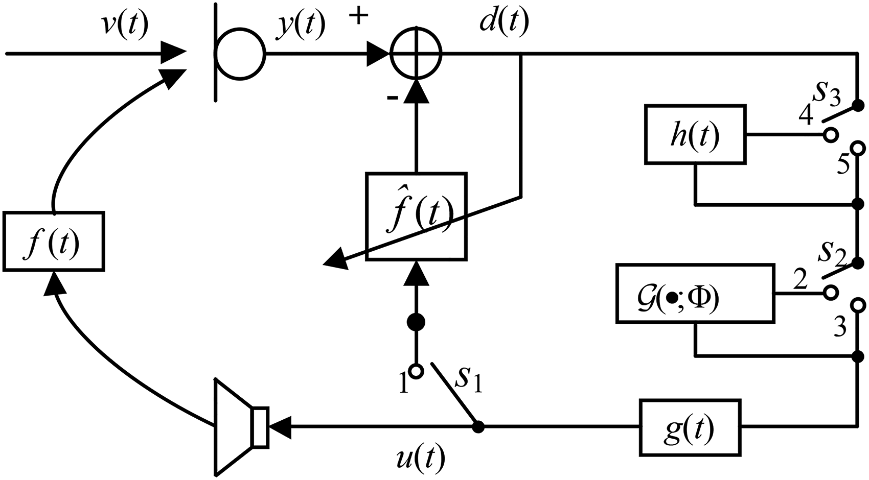
Signal flowchart of a hearing aid. There are three interlinked switches, $s_{1}$ , $s_{2}$ , and $s_{3}$ . When $s_{1}$ is not connected with 1, $s_{2}$ is connected to 3, and $s_{3}$ is connected to 5, so no signal processing is used to avoid instability. When $s_{1}$ is connected to 1, AFC is turned on. When $s_{3}$ is connected to 4, FS and/or gain-control approaches are used. When $s_{2}$ is connected to 2, DeepMFC is used for feedback control. AFC: adaptive feedback cancellation; FS: frequency shifting.

Different types of approaches often have different underlying assumptions, and the performance of a given approach may be poor when the assumptions are not satisfied or are poorly approximated. When Schroeder (1964) theoretically and experimentally studied the additional stable gain (ASG; the amount by which the gain can be increased before instability occurs) provided by FS, the intended application was in public address systems, for which it was assumed that feedback was caused only by the reverberant sound field. However, for hearing aids, the direct sound from the receiver to the microphone and early reflections from nearby surfaces are usually dominant. Because FS does not require any assumptions about the type of sound source, it works for both speech and music, although music quality may be somewhat degraded because annoying beats are often produced when open-fit hearing aids are used and the sound reaching the eardrum is a mixture of sound leaking through the open fitting and sound produced by the hearing aid (Moore, 2016).

For AFC, it is often assumed that the feedback path between the receiver and microphone is time-invariant or only slowly time-varying (Bustamante et al., 1989; Kates, 1991; Guo et al., 2012). When the feedback path changes rapidly, for example, when the hearing-aid user moves close to a reflecting surface, it takes some time to track this change and howling may occur during the convergence stage. Although the convergence rate can be improved by properly choosing the step size when recursively updating the filter coefficients of the AFC (Rotaru et al., 2012), instability may still occur for a short time.

AFC systems suffer from bias in the estimation of the feedback signal when the sound source is spectrally colored (Kates, 1991; Hellgren, 2002; Spriet et al., 2005; Guo et al., 2012). This is especially serious when the sound source is music, since the AFC may cancel steady tones instead of removing the feedback signal. However, speech is also a spectrally colored signal, leading to problems with estimation bias. To deal with this, speech can be spectrally flattened (whitened) with a time-varying low-order infinite impulse response filter, using a speech-production model (Quatieri, 2006). This approach called the prediction error method (PEM) was combined with an AFC method (PEM–AFC) by Spriet et al. (2005). When the sound source was speech, PEM–AFC performed much better than AFC approaches without whitening, in terms of convergence rate, estimation bias, and the amount of ASG. However, as demonstrated by Guo et al. (2013), PEM–AFC did not outperform AFC approaches without whitening when the sound source was music. This may be because music cannot be whitened using the prediction error method of Spriet et al. (2005).

Gain-control-based feedback suppression approaches (Patronis, 1978; Foley, 1989; Waterschoot & Moonen, 2010) detect howling components in the first stage and gain reduction is then applied to subbands containing howling components. The performance of gain-control approaches depends on the accuracy of howling detection (Waterschoot & Moonen, 2010). This leads to problems with music, since the tonal components in music may be identified as howling components, resulting in gain reductions at many frequencies and a degradation of sound quality.

A deep-learning framework for feedback control called DeepMFC was recently proposed by Zheng, Wang et al. (2022). DeepMFC was primarily intended to reduce the artifacts associated with feedback reduction when a system was working with a gain just below the maximum stable gain, a state referred to as a marginally stable gain. These artifacts include spectral coloration, whereby the gain is higher than desired at frequencies where the gain is only slightly below the maximum stable gain, and short whistles occurring when the feedback path changes. However, DeepMFC also increased the maximum stable gain. Unlike the above-mentioned approaches, DeepMFC is data-driven. DeepMFC was shown to outperform non-data-driven approaches in terms of objective and subjective measures when the sound source was speech. In DeepMFC, the complex spectrum of the microphone signal is mapped directly to the complex spectrum of the receiver signal using a pre-trained deep complex neural network denoted $G (∙, Φ)$ with the structure proposed by Tan & Wang (2020), as shown in Figure 1. The receiver signal is then obtained using the overlap-add or overlap-save method. Because of this direct mapping, the ASG produced by DeepMFC cannot be measured or calculated directly. However, it was shown by Zheng, Wang et al. (2022) that DeepMFC did not significantly reduce scores based on the objective measure ”perceptual evaluation of speech quality” (PESQ)² (Rix et al., 2001), even when the gain margin in decibels³ decreased from about $3$ dB to $- 5$ dB. It was not evaluated how well DeepMFC works when the sound source was music.

This paper had three purposes. The first was to evaluate DeepMFC in simulated closed-loop systems with measured feedback paths for both music and speech using different models trained with different materials and using both objective and subjective measures. The second was to estimate the ASG provided by DeepMFC using the hearing-aid speech quality index version 2 (HASQI-V2) proposed by Kates & Arehart (2014) and the hearing-aid audio quality index (HAAQI) proposed by Kates & Arehart (2016). The third purpose was to clarify the way in which DeepMFC works.

Methods

DeepMFC Models

Zheng, Wang et al. (2022) proposed a data-driven feedback control approach, called DeepMFC. Using both objective metrics and listening tests DeepMFC was shown to perform better than several effective and representative approaches, including FS, AFC, and PEM–AFC, when training was done using speech in background noise and the sound source for testing was speech in quiet or in noise. For the present paper, a DeepMFC model with the same architecture as in Zheng, Wang et al. (2022) was retrained, because we found that performance was improved when the length of the simulated feedback paths was increased from about 3 ms to about 15 ms. The model that was re-trained with speech is denoted DeepMFC(1). In total, 10,000 feedback paths with lengths randomly selected from 200 to 300 samples for the sampling rate of 16 kHz were simulated. When training DeepMFC(1), the WSJ0-SI84 speech corpus (Paul & Baker, 1992) was used. In total, 40,000 utterances spoken by 76 speakers were randomly selected and each utterance was mixed with a noise clip randomly chosen from the DNS-Challenge data set (Reddy et al., 2021) at a signal-to-noise ratio randomly selected from 5, 10, 15, and 20 dB. Each noisy mixture was used together with one randomly selected simulated feedback path to generate the closed-loop receiver signal when the closed-loop system performed in marginal stable gain states (Zheng, Wang, et al., 2022). The corresponding open-loop receiver signal with the same clean utterance as the sound source was generated and paired with the closed-loop receiver signal. Note that the training target was clean speech. Thus, DeepMFC(1) was intended both to control feedback and to reduce noise. In total, 40,000 paired speech signals were included in the speech training data set. The paired speech validation data set was generated using 2400 utterances spoken by the same speakers as for the training data set. For both the speech training and validation data sets, the duration of each utterance was cut to 4 s. Note that DeepMFC(1) becomes a deep noise reduction (DeepNR) model when each noisy mixture is used as the receiver signal and paired with its corresponding clean speech to create the training data set. Zheng, Wang et al. (2022) showed that DeepNR performed worse than DeepMFC(1) in handling feedback. Although DeepNR suppressed howling components, it did not solve the coloration problem effectively. Thus DeepNR will not be discussed further in this paper.

A second DeepMFC model, denoted DeepMFC(2), was trained to control feedback when the sound source was music. For this purpose, the sound sources used for the training and validation data sets were taken from the synthesized Lakh data set, denoted Slakh, provided by Manilow et al. (2019). Slakh was designed for the evaluation of music source separation approaches, and its first version, Slakh2100, had 2100 instrumental pieces with a total duration of about 145 hours. In total, 80,000 clips randomly cut from Slakh2100 were used as the source signals for training. One simulated feedback path was randomly selected and used together with each clip to generate the closed-loop receiver signal. The corresponding open-loop receiver signal with the same music clip was generated and paired with the closed-loop receiver signal. In total, 80,000 paired clips were included in the music training data set. The paired music validation data set was generated in the same way as the paired music training data set, using 2400 clips randomly cut from Slakh2100. For both the training and validation data sets, each music clip was cut to 4 s.

A third DeepMFC model, denoted DeepMFC(3), was trained to appropriately process either speech or music. While DeepMFC(1) was primarily intended for feedback control, it also had the effect of reducing background noise. As denoising may seriously degrade music quality, only clean speech $v (n)$ was used for training and validation of DeepMFC(3). A randomly selected speech clip was used together with one randomly selected simulated feedback path to generate 40,000 pairs for training and 2400 pairs for validation. These materials were combined with the training and validation materials used for DeepMFC(2) to train the DeepMFC(3) model. Because the DeepMFC(3) model was trained using both speech and music, it was expected that this model would achieve intermediate performance for both speech and music, while DeepMFC(1) might perform better for speech and DeepMFC(2) might perform better for music.

Comparison Control Approaches, Stimuli, and Procedure

Feedback Control Approaches

In addition to the three DeepMFC models, three more traditional feedback-control methods, FS, PEM–AFC, and their combination, denoted FS+PEM–AFC, were implemented and evaluated. As demonstrated by Zheng, Wang et al. (2022), performance was improved when DeepMFC was combined with PEM–AFC when the gain margin in decibels was set to be negative. For completeness, we also evaluated the combination of two traditional approaches and DeepMFC, specifically FS+DeepMFC and PEM–AFC+DeepMFC. In summary, the following 10 feedback-control approaches, including five single-stage and five two-stage approaches were used and compared:

FS: the approach proposed by Schroeder (1964) was used with a frequency shift of 10 Hz.

PEM–AFC: the approach proposed by Spriet et al. (2005) was used. The fixed step size of the normalized least mean square algorithm for updating the feedback path was set to 0.005. To improve its performance for music, when estimating the feedback path a time-invariant high-pass 3-tap finite impulse response (FIR) filter was applied to the output signal of PEM–AFC $d (t)$ and the receiver signal $u (t)$ , with filter coefficients 1, $- 1.8$ , and 0.81, as proposed by Hellgren (2002). It should be emphasized that this FIR filter was used only to improve the estimation of the feedback path; it was not applied to the signals themselves. As in Lee et al. (2017), the filter length of PEM–AFC was set to 100, using a sample rate of 16 kHz. Two initialization methods were assessed. For one, the initial feedback path was obtained by averaging several measured feedback paths. This is denoted PEM–AFC; for the other, the coefficients of the initialized feedback path were all set to 0. This is denoted PEM–AFC(0).

DeepMFC(1): this model was expected to give the best performance when the source was speech, because it suppresses noise and reduces feedback problems simultaneously.

DeepMFC(2): this model was expected to give better performance than DeepMFC(1) when the source was music.

DeepMFC(3): this model was expected to give moderate performance for both speech and music.

PEM–AFC+FS: the output signal from PEM–AFC was further processed using FS. As shown by Guo et al. (2013) and Zheng, Wang et al. (2022), FS improved the performance of PEM–AFC when the gain margin in decibels was negative.

FS+DeepMFC(1): after performing FS the signal was further processed using DeepMFC(1) when the source was speech. While DeepMFC(1) was not trained using signals with FS, it has been shown that DeepMFC is robust to both linear and non-linear processing of the signal (Zheng, Wang, et al., 2022).

PEM–AFC+DeepMFC(1): after performing PEM–AFC, the signal was further processed using DeepMFC(1) when the source was speech.

FS+DeepMFC(3): after performing FS the signal was further processed using DeepMFC(3) when the source was music. Note that DeepMFC(2) was not used. Although preliminary experiments showed that it achieved better performance than DeepMFC(1) for music, DeepMFC(2) gave worse performance than DeepMFC(3) for music. This may have occurred because Slahk2100 (Manilow et al., 2019) contains only instrumental pieces, while the test materials contained both musical instruments and singing voices.

PEM–AFC+DeepMFC(3): the output from PEM–AFC was further processed using DeepMFC(3) when the source was music.

All the above-mentioned approaches were run using the simulated closed-loop system shown in Figure 1. By changing the status of the three switches, one or various combinations of feedback control approaches could be implemented. When

s_{1}

is not connected to 1, and

s_{2}

and

s_{3}

are connected to 2 and 5, respectively, only DeepMFC is used for feedback control. When

s_{1}

is connected to 1, PEM–AFC is turned on. When

s_{3}

is connected to 4 instead of 5, FS is used in the feedforward path. When

s_{2}

is connected to 3 instead of 2, DeepMFC is by-passed.

Stimulus Generation

When training all DeepMFC models, only simulated feedback paths were used. The simulation method was the same as described by Zheng, Wang et al. (2022). When testing the various feedback-control approaches, only feedback paths measured using a hearing aid (Lee et al., 2017)⁴ were used in the simulated closed-loop system. In this way, the feedback paths used for testing were unseen during training. The length of each measured feedback path was 263 samples using a sampling rate of 16 kHz.

It is well known that better performance of deep-learning approaches is often achieved when the source for the test, $v (t)$ , is included in the training stage. To avoid this, utterances spoken by the remaining seven unseen speakers in the WSJ0-SI84 corpus were randomly chosen as the source signals to test the DeepMFC models when the source was speech. The duration of each utterance in the WSJ0-SI84 corpus was $<$ 10 s, so several utterances were concatenated to form 30-s utterances. Twelve such utterances were used for testing. When the source was music, 12 clips of music downloaded from a music player app were used as $v (t)$ in Figure 1. These 12 clips included four genres, Jazz, Classical, Choir, and Pop, and each type contained three clips. For both speech and music, the duration of each source in the test stage was 30 s.

With the measured feedback paths and different types of sound sources, the feedback-control approaches were run one by one in the closed-loop systems and the receiver signals were recorded for objective and subjective measures. To measure performance with different prescribed gains, the value $K$ in the forward path, with $g (t) = K δ (t)$ , was increased to give gain margins in decibels ranging from $- 14$ to 0 dB in 0.5 dB steps and from 0 to 4 dB in 1 dB steps.

For each approach, $12 \times 33 = 396$ speech utterances and 396 music samples were used for evaluation, because the number of speech utterances or music clips was 12 and the number of $K$ values was 33.

Objective Quality Assessment

Objective quality measures often give inconsistent results when applied to speech and music signals (Torcoli et al., 2021). For that reason, separate measures are needed for speech and music. The wideband PESQ metric proposed by Rix et al. (2001) is often used to evaluate the quality of unprocessed and processed speech signals for NH listeners, because PESQ scores are usually highly correlated with subjective scores for speech quality for these listeners. Note that PESQ was originally designed to measure speech quality in the context of speech coding, but it has since been used to assess the influence of more types of distortions, including noise (Hu & Loizou, 2007), reverberation (Naylor & Gaubitch, 2010), and acoustic feedback (Schepker et al., 2020). However, the PESQ metric is not designed to take into account the effects of hearing loss or of hearing-aid signal processing. Here, in addition to PESQ, the HASQI-V2 (Kates & Arehart, 2014) was used to evaluate speech quality, while the HAAQI (Kates & Arehart, 2016) was used to evaluate music quality. HAAQI scores are more highly correlated than HASQI-V2 scores with subjective ratings of music sound quality (Kates & Arehart, 2016).

The HASQI-V2 and HAAQI metrics can be used to simulate both NH and hearing loss. Both require the audiometric thresholds of the simulated listener to be entered. If the audiometric thresholds are specified as 0 dB hearing level (HL) at all frequencies, the metrics use a model of auditory processing to give estimates of sound quality for listeners with NH. If some of the audiometric thresholds are specified as $>$ 0 dB HL, corresponding to a hearing loss, the auditory model is modified so as to take into account some of the typical consequences of hearing loss, such as reduced frequency selectivity (Glasberg & Moore, 1986) and reduced compression in the cochlea (Moore et al., 1996). The two metrics give the option of applying frequency-dependent gain to compensate for the reduced audibility produced by the hearing loss, based on the National Acoustic Laboratories’ nonlinear fitting procedure-Revised (NAL-R) method (Byrne & Dillon, 1986). That option was used here because Arehart et al. (2010, 2011) showed that speech or music filtered using the NAL-R method based on individual thresholds yielded the highest quality for hearing-impaired listeners. Note that both the reference signal and the processed signal were filtered using the NAL-R method when calculating HASQI-V2 and HAAQI values. The software for calculating HASQI-V2 and HAAQI scores was used with the default setting that a signal with a root-mean-square (RMS) value of 1 has a level of 65 dB SPL. Each signal was normalized to have an RMS value of 1, so the effective input level was 65 dB SPL. The NAL-R recommended gains are suitable for this level.

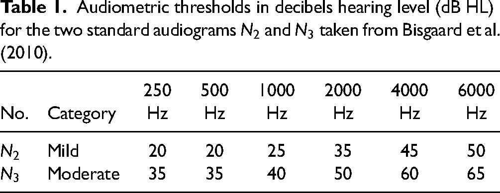
Only mild and moderate hearing losses were simulated. Bisgaard et al. (2010) divided standard audiograms into two groups: a flat and moderately sloping group, and a steeply sloping group. The first group included seven audiograms characterizing different degrees of hearing loss, while the second group had three audiograms with different degrees of hearing loss. Here, two standard audiograms $N_{2}$ and $N_{3}$ with mild and moderate sloping hearing loss, respectively, were used, as shown in Table 1. Note that HASQI-V2 and HAAQI only require as input the audiometric threshold at six frequencies: 250, 500, 1000, 2000, 4000, and 6000 Hz.

Table 1.

Audiometric thresholds in decibels hearing level (dB HL) for the two standard audiograms $N_{2}$ and $N_{3}$ taken from Bisgaard et al. (2010).

No.	Category	250 Hz	500 Hz	1000 Hz	2000 Hz	4000 Hz	6000 Hz
$N_{2}$	Mild	20	20	25	35	45	50
$N_{3}$	Moderate	35	35	40	50	60	65

For each approach and each type of source, an average score for each objective quality measure was calculated across all clips for a specific value of the gain margin, giving 33 average scores for speech and 33 average scores for music.

Subjective Quality Assessment

Paired comparisons were used to estimate subjective preference scores. This was done separately for speech and music signals. Fifteen participants with self-assessed NH were tested. Their ages ranged from 20 to 52 years. All were native Chinese speakers. Since the experiment involved listening to stimuli presented at safe sound levels, in accordance with local regulations, no ethical approval was required.

For speech, the conditions that were compared were: unprocessed, PEM–AFC, DeepMFC(1), and PEM–AFC+DeepMFC(1), giving six pairs. For music, the conditions that were compared were: unprocessed, PEM–AFC, DeepMFC(3), and PEM–AFC+DeepMFC(3), again giving six pairs. Gain margins of 0, $- 5$ and $- 10$ dB were used.

Stimuli were presented diotically via headphones (Sennheiser HD202, Wedemark, Germany). The levels of all stimuli were adjusted to give the same peak level, and the overall level was adjusted separately for each participant until it was judged to be at the most comfortable level. Each participant was asked to compare all six pairs of approaches using a gain margin of 0 dB. For the negative gain margins, only conditions that did not lead to instability were tested. Thus, three pairs of approaches (PEM–AFC versus DeepMFC, PEM–AFC versus PEM–AFC+DeepMFC, and DeepMFC versus PEM–AFC+DeepMFC) were compared using a gain margin of $- 5$ dB, and one pair of approaches (DeepMFC versus PEM–AFC+DeepMFC) was compared using a gain margin of $- 10$ dB.

Each participant was presented with five pairs of utterances for each pair of approaches and each gain margin and selected one of the three options after the presentation of each pair: first better, second better, or equal. The order of presentation of the approaches within a pair was random. When approach A was selected as the better one, one point was assigned to approach A, and zero to approach B, and vice versa. When equal was selected, “equal” was assigned one point. The points were summed for each approach and the total was divided by 75 and multiplied by 100 to obtain a preference score as a percentage.

Results

Speech Quality for Simulated NH Listeners

Figures 2 and 3 show the PESQ and HASQI-V2 scores, respectively, assuming NH listeners for HASQI-V2. Among the feedback-control approaches, only AFC-based approaches explicitly estimate the feedback path. When the feedback path is simulated and time-invariant, as here, the ASG in decibels resulting from the use of AFC can be computed by subtracting the maximum stable gain without AFC from that with AFC. For other types of feedback-control approaches, the ASG is more difficult to determine, because the maximum stable gain with feedback control cannot be computed directly. 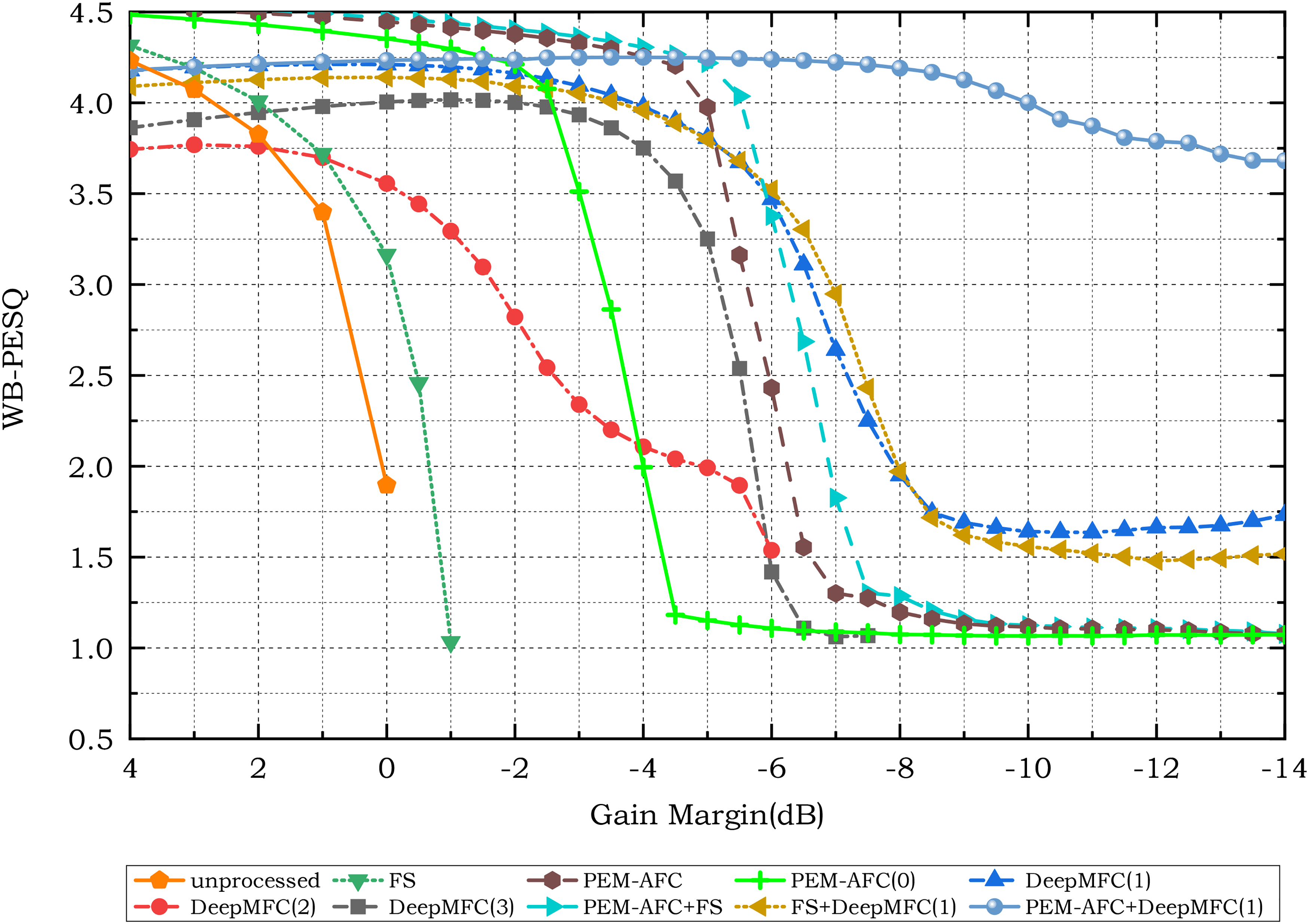To estimate the ASG of the different feedback-control approaches, the gains giving a PESQ score $> 3.0$ or a HASQI-V2 score $> 0.8$ were chosen as corresponding approximately to the maximum stable gain and were used to estimate the ASG.⁵ Lee et al. (2017) also used the HASQI-V2 score to determine the maximum stable gain of feedback-control approaches and also used 0.8 as the criterion value. Table 2 presents the estimated ASG in decibels for the different feedback-control approaches for speech. When the HASQI-V2 score was <0.8 for all gain margins, the estimated ASG in decibels is not shown.

Figure 2.

Wideband perceptual evaluation of speech quality (WB-PESQ) scores for unprocessed and processed speech using different feedback-control approaches.

Figure 3.

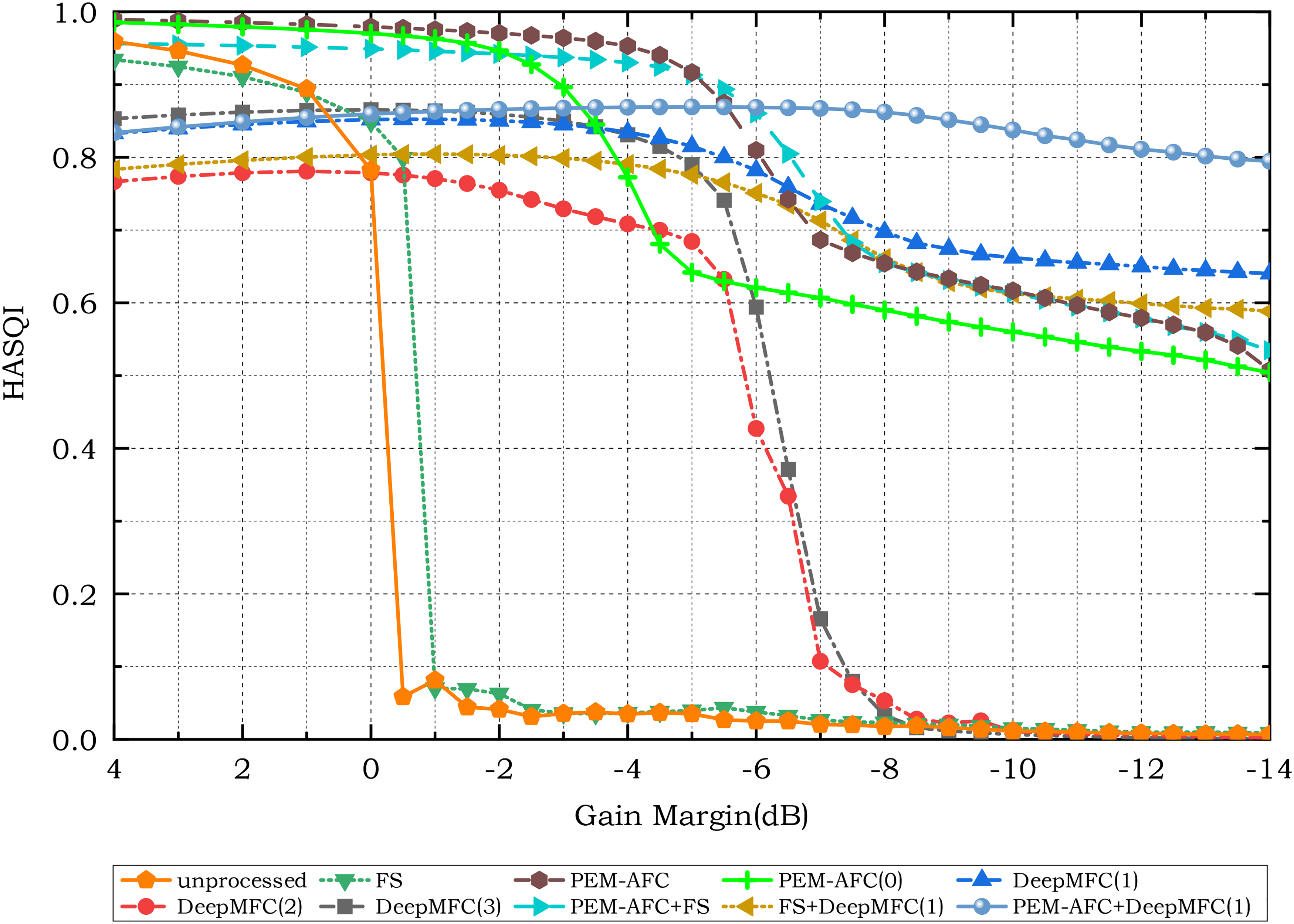
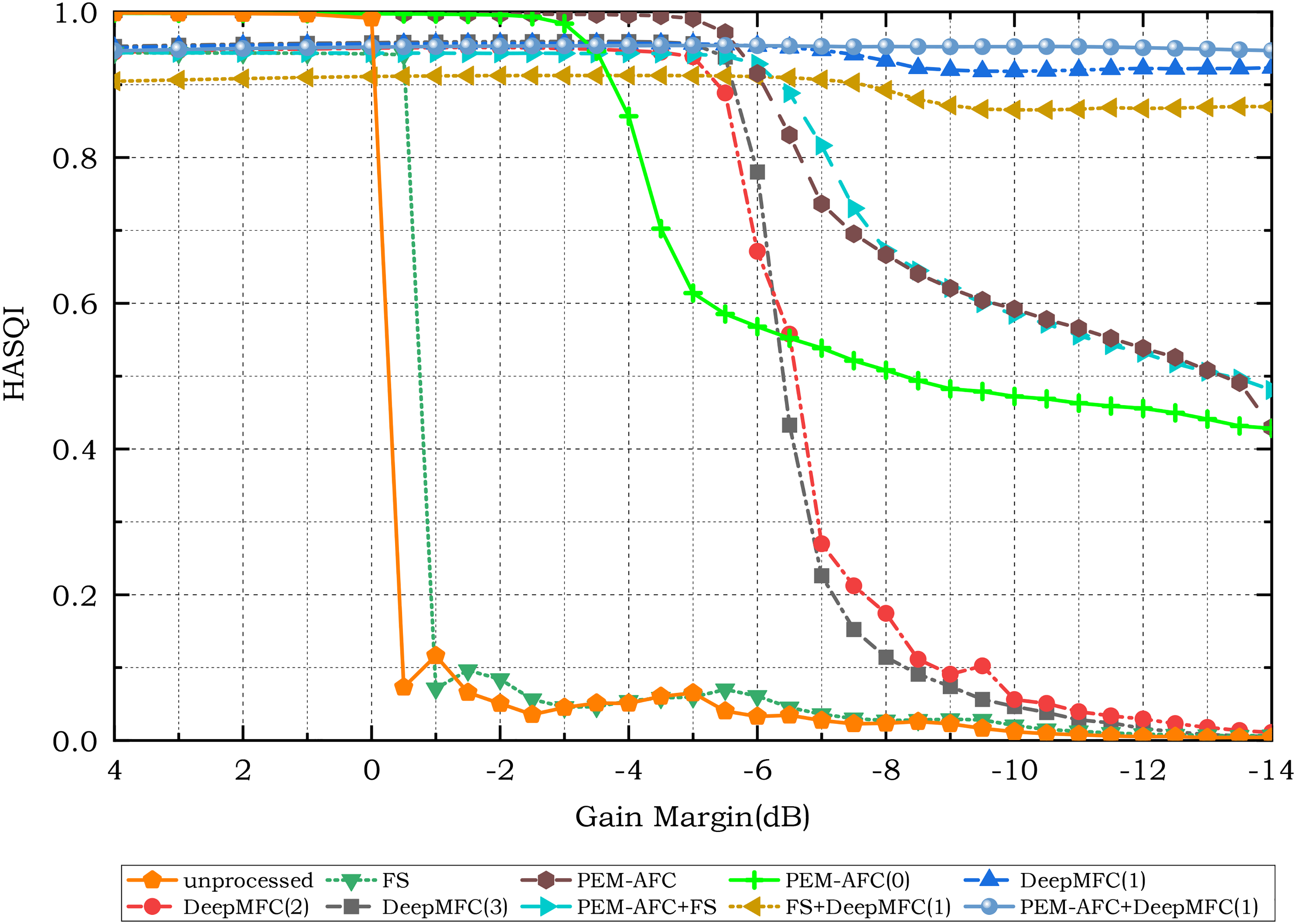
Hearing-aid speech quality index version 2 (HASQI-V2) scores for unprocessed and processed speech using different feedback-control approaches, assuming normal-hearing listeners.

Table 2.

Estimated ASG (in dB) of the feedback-control approaches using the HASQI-V2 score for speech. The estimated ASG using the WB-PESQ score is shown in brackets for the simulated NH listeners.

Approach	NH	Mild (N2)	Moderate (N3)
Unprocessed	−1.0 (−1.0)	0.0	−1.0
FS	0.0 (0.0)	0.5	0.5
PEM–AFC	6.0 (5.5)	6.5	6.5
PEM–AFC(0)	3.5 (3.0)	4.0	4.0
DeepMFC(1)	5.0 (6.5)	8.5	14.0
DeepMFC(2)	−(1.5)	5.5	5.5
DeepMFC(3)	4.5 (3.0)	5.5	5.5
PEM–AFC+FS	6.5 (6.0)	7.0	7.0
FS+DeepMFC(1)	−(6.5)	7.0	14.0
PEM–AFC+DeepMFC(1)	13.0 (14.0)	14.0	14.0

ASG: additional stable gain; HASQI-V2: hearing-aid speech quality index version 2; WB-PESQ: wideband perceptual evaluation of speech quality; NH: normal hearing; FS: frequency shifting; PEM: prediction error method; AFC: adaptive feedback cancellation.

Without any feedback control, both WB-PESQ and HASQI-V2 scores worsened dramatically when the gain margin in decibels changed from positive to negative values, because the system became unstable and howling occurred. With FS alone, the ASG was about 0 dB⁶, consistent with the theoretical analysis of Zheng et al. (2016) and the experimental results of Berdahl & Harris (2010). For PEM–AFC, which was initialized by averaging several measured feedback paths, the ASG was about 6 dB, which is 2 to 3 dB higher than the ASG for PEM–AFC(0). This indicates that appropriate initialization of the AFC is important. The combination of FS and PEM–AFC improved the ASG relative to PEM–AFC alone, but the improvement was <1 dB.

Of the three versions of DeepMFC, DeepMFC(2) performed the most poorly; the HASQI-V2 score was lower than the criterion value of 0.8 for all gain margins. This indicates that using only music clips for training was not sufficient to give substantial ASG for speech. The combination of FS and DeepMFC(1) did not markedly affect the ASG, while the combination of PEM–AFC and DeepMFC(1) yielded the highest ASG of 13 to 14 dB. DeepMFC(1) yielded the highest ASG among the individual feedback control approaches.

Speech Quality for Simulated Hearing-Impaired Listeners

Figures 4 and 5 show the HASQI-V2 scores for simulated hearing-impaired listeners with mild (N2) and moderate (N3) hearing loss, respectively. The same threshold as used for the simulated NH listeners, 0.8, was used to determine the maximum stable gain of the different feedback-control approaches for the simulated hearing-impaired listeners. Comparison of Figures 4 and 5 with Figure 3 shows that for almost all of the feedback-control approaches the maximum stable gain increased with increasing hearing loss, as can also be seen from Table 2. For example, the maximum stable gain for DeepMFC(1) increased from 6 dB for the simulated NH listeners to 8.5 dB for the listeners with simulated mild hearing loss (N2) and to over 14 dB for the listeners with simulated moderate hearing loss (N3). For the latter, DeepMFC(1) alone performed very well, and combining it with PEM–AFC led to only slightly higher HASQI-V2 scores. In contrast, for both the simulated NH listeners and simulated listeners with mild hearing loss, the combination of PEM–AFC and DeepMFC(1) led to a much higher maximum stable gain than for either method alone. The finding that HASQI scores were higher for simulated hearing-impaired listeners than for simulated NH listeners is consistent with the results presented by Kates & Arehart (2022). As explained by Kates & Arehart (2022), these higher scores may have occurred because the simulated hearing-impaired listeners were less sensitive than the simulated NH listeners to signal degradations such as increased gain at certain frequencies (coloration), owing to the simulated reduced frequency selectivity of the former. Also, for the simulated hearing-impaired listeners, some distortion spectral components would have had levels below the hearing threshold, and thus would not be perceived (Tan & Moore, 2008).

Figure 4.

Hearing-aid speech quality index version 2 (HASQI-V2) scores for unprocessed and processed speech using different feedback-control approaches, assuming hearing-impaired listeners with mild hearing loss (N2).

Figure 5.

Music Quality for Simulated NH Listeners

Figure 6 shows the HAAQI scores for simulated NH listeners for the unprocessed and processed music signals using the different feedback control approaches. HAAQI scores were generally lower than HASQI scores and so a lower criterion, 0.6, was chosen as the threshold indicating the maximum stable gain for each approach. Informal listening tests confirmed that music quality was relatively high when the HAAQI score was above 0.6. Table 3 shows the estimated ASG in decibels of each feedback-control approach for music. When the HAAQI score was <0.6 for all gain margins, the estimated ASG is not shown.

Figure 6.

Hearing-aid audio quality index (HAAQI) scores for unprocessed and processed music signals using different feedback control approaches for simulated normal-hearing listeners.

Table 3.

As Table 2 but for music.

Approach	NH	Mild (N2)	Moderate (N3)
Unprocessed	0.0	0.0	0.0
FS	0.5	0.5	0.5
PEM–AFC	10.0	11.5	13.5
PEM–AFC(0)	7.0	9.0	10.0
DeepMFC(1)	-	−2.0	6.0
DeepMFC(2)	4.5	6.5	7.0
DeepMFC(3)	5.0	6.0	6.0
PEM–AFC+FS	10.5	11.5	14.0
FS+DeepMFC(3)	5.5	6.5	6.5
PEM–AFC+DeepMFC(3)	9.5	13.5	14.0

NH: normal hearing; FS: frequency shifting; PEM: prediction error method; AFC: adaptive feedback cancellation.

Of the single approaches, PEM–AFC achieved the highest ASG (about 10 dB), and its combination with DeepMFC(3) gave nearly the same ASG. PEM–AFC(0) yielded much poorer HAAQI scores than PEM–AFC, the ASG of PEM–AFC(0) being only about 7 dB. This again shows the importance of initialization. With initialization based on measured feedback paths, PEM–AFC converged rapidly, while if all adaptive filter coefficients were initially set to 0, PEM–AFC converged slowly and instability occurred at the beginning of the adaptation period or when the feedback path changed. For DeepMFC(2) and DeepMFC(3), the ASG was about 5 dB. DeepMFC(3) performed only slightly better than DeepMFC(2). DeepMFC(1) performed the most poorly among the three deep-learning approaches, and it failed to increase the maximum stable gain. More seriously, DeepMFC(1) degraded HAAQI scores markedly even when the closed-loop system worked in a stable state. This confirms the importance of using matched training and testing conditions⁷ for deep learning-based approaches. FS yielded an ASG <1 dB for music, consistent with the result for speech.

Music Quality for Simulated Hearing-Impaired Listeners

Figures 7 and 8 show the HAAQI scores for the simulated listeners with mild and moderate hearing loss, respectively. DeepMFC(1) yielded the lowest HAAQI scores when the gain margin was high, indicating that it degraded sound quality. This again confirms the importance of using music for training when the source for evaluation is music rather than speech. As can be seen in Table 3, the highest ASG values were obtained with PEM–AFC and the combination of PEM–AFC and DeepMFC(3). HAAQI scores for PEM–AFC were higher for the simulated hearing-impaired listeners than for the simulated NH listeners. The ASG for PEM–AFC(0) was about 3 dB smaller than that for PEM–AFC. DeepMFC(2) and DeepMFC(3) yielded ASGs of 6 to 7 dB for the N2 and N3 listeners. FS gave a small ASG value of 0.5 dB.

Figure 7.

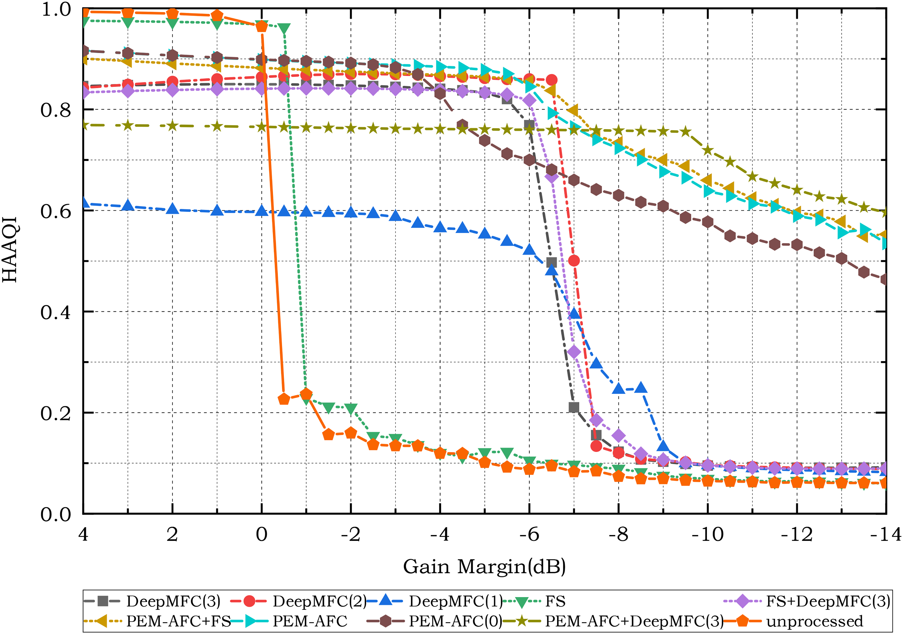
Hearing-aid audio quality index (HAAQI) scores for unprocessed and processed music signals using different feedback control approaches for simulated listeners with mild hearing loss.

Figure 8.

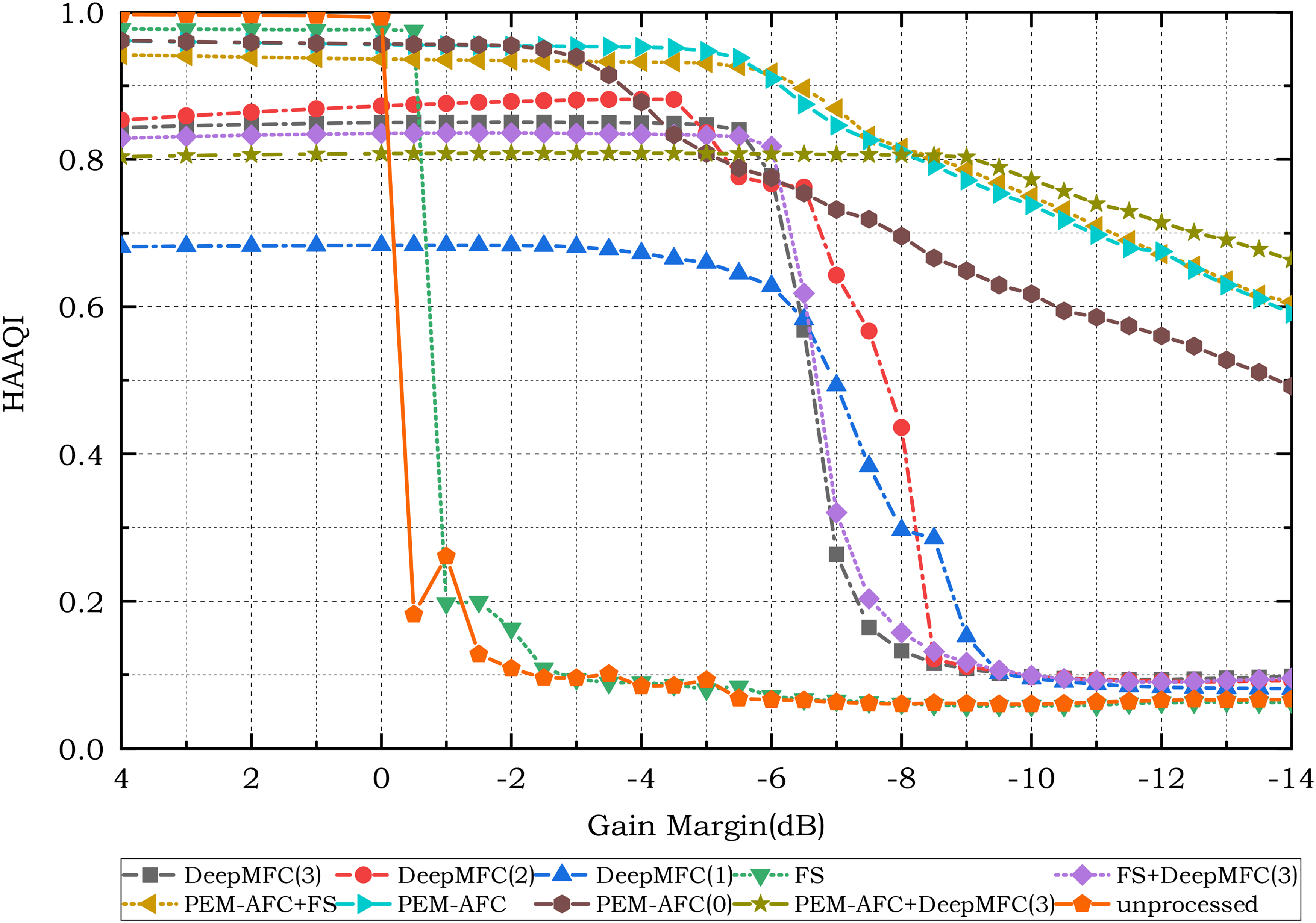
Hearing-aid audio quality index (HAAQI) scores for unprocessed and processed music signals using different feedback control approaches for simulated listeners with moderate hearing loss.

Comparison of Figure 6 with Figures 7 and 8 shows that HAAQI scores for unprocessed music differed for simulated NH and hearing-impaired listeners. When the gain margin was reduced from 4 dB to 0 dB, the HAAQI scores remained above 0.95 for the simulated hearing-impaired listeners, while the scores decreased from slightly over 0.9 to below 0.8 for the simulated NH listeners. The higher HAAQI scores for the simulated hearing-impaired listeners shown in Figures 7 and 8 are consistent with the HASQI scores in Figures 4 and 5. These higher scores probably occurred for the same reasons as discussed earlier, namely reduced sensitivity of hearing-impaired listeners to signal degradations.

Results of the Listening Test for Speech

Table 4 presents the results of the listening test for speech. When the gain margin was set to 0 dB, both PEM–AFC and DeepMFC(1) were clearly preferred over the unprocessed signals. DeepMFC(1) was preferred over PEM–AFC, and the difference was small but significant ( $χ^{2} = 10.9$ , $p = 0.004$ ), about 59 $%$ of ratings being “equal.” For the gain margin of 0 dB, DeepMFC(1) and the combination PEM–AFC+DeepMFC(1) were equally preferred. This indicates that DeepMFC(1) alone worked well enough to make its combination with PEM–AFC unnecessary, consistent with our previous study, Zheng, Wang et al. (2022). The combination PEM–AFC+DeepMFC(1) was clearly preferred over PEM–AFC. For the gain margin of 0 dB, except for the two comparisons already described, PEM–AFC versus DeepMFC(1) and DeepMFC(1) versus PEM–AFC+DeepMFC(1), all comparisons gave significant differences at $p < 0.0001$ .

Table 4.

Subjective preference scores for speech.

Gain margin	0 dB	$- 5$ dB	$- 10$ dB
Unprocessed	2.7%	–	–
PEM–AFC	97.3%	–	–
Equal	0.0%	–	–
Unprocessed	2.7%	–	–
DeepMFC(1)	97.3%	–	–
Equal	0.0%	–	–
Unprocessed	1.3%	–	–
PEM–AFC+DeepMFC(1)	98.7%	–	–
Equal	0.0%	–	–
PEM–AFC	12.0%	65.3%	–
DeepMFC(1)	29.3%	33.3%	–
Equal	58.7%	1.3%	–
PEM–AFC	0.0%	0.0%	–
PEM–AFC+DeepMFC(1)	45.3%	93.3%	–
Equal	50.7%	6.7%	–
DeepMFC(1)	2.7%	0.0%	1.3%
PEM–AFC+DeepMFC(1)	2.7%	97.3%	97.3%
Equal	94.7%	2.7%	1.3%

PEM: prediction error method; AFC: adaptive feedback cancellation.

For the gain margin of $- 5$ dB, the combination PEM–AFC+DeepMFC(1) was clearly preferred over PEM–AFC alone and DeepMFC(1) alone, and PEM–AFC was preferred over DeepMFC(1). The latter effect might be a consequence of the fact that DeepMFC(1) was trained using only positive gain margins. For the gain margin of $- 10$ dB, the combination PEM–AFC+DeepMFC(1) was clearly preferred over DeepMFC(1) alone. Although PEM–AFC was not used in training DeepMFC(1), the results confirm that DeepMFC(1) can be used as a post-processing module to improve the performance of PEM–AFC, consistent with our previous study Zheng, Wang et al. (2022).

Results of the Listening Test for Music

Table 5 shows the results of the listening test for music. For the gain margin of 0 dB, PEM–AFC was preferred over DeepMFC(3) ( $χ^{2} = 9.0$ , $p = 0.011$ ) and over the combination PEM–AFC+DeepMFC(3) ( $χ^{2} = 19.7$ , $p < 0.0001$ ), which differs from the results for speech. This may have happened because the music stimuli were distorted by DeepMFC(3). When the gain margin was set to $- 5$ dB, the combination PEM–AFC+DeepMFC(3) was clearly preferred over PEM–AFC and DeepMFC(3), and when the gain margin was set to $- 10$ dB the combination PEM–AFC+DeepMFC(3) was clearly preferred over DeepMFC(3)(all $p < 0.0001$ ). The preference for PEM–AFC+DeepMFC(3) over PEM–AFC for the $- 5$ dB gain margin is inconsistent with the HAAQI scores for simulated NH listeners shown in Figure 6. This suggests that HAAQI scores do not always correspond to subjective preferences. This discrepancy might have occurred because participants paid more attention to the howling components of music processed by PEM–AFC at the beginning of the adaptation period than to the distortion caused by DeepMFC(3) during the ongoing part of the stimulus. Overall, the listening test results indicate that, for negative gain margins, preferences were greatest for the combination PEM–AFC+DeepMFC(3), perhaps because PEM–AFC was very effective in canceling feedback while DeepMFC(3) was effective in reducing artifacts.

Table 5.

As Table 4 but for music.

Gain Margin	0 dB	$- 5$ dB	$- 10$ dB
Unprocessed	1.3%	–	–
PEM–AFC	98.7%	–	–
Equal	0.0%	–	–
Unprocessed	0.0%	–	–
DeepMFC(3)	98.7%	–	–
Equal	1.3%	–	–
Unprocessed	4.0%	–	–
PEM–AFC+DeepMFC(3)	92.0%	–	–
Equal	4.0%	–	–
PEM–AFC	29.3%	76.0%	–
DeepMFC(3)	13.3%	20.0%	–
Equal	57.3%	4.0%	–
PEM–AFC	28.0%	6.7%	–
PEM–AFC+DeepMFC(3)	6.7%	89.3%	–
Equal	65.3%	4.0%	–
DeepMFC(3)	5.3%	1.3%	0.0%
PEM–AFC+DeepMFC(3)	18.7%	94.7%	100.0%
Equal	76.0%	4.0%	0.0%

PEM: prediction error method; AFC: adaptive feedback cancellation.

Characterization of How DeepMFC Works for Speech and Music

With the speech signals, DeepMFC(1) performed very well for all types of simulated listeners regardless of the degree of hearing loss and it also performed well in the subjecti6ve listening test. The ASG of DeepMFC(1) was up to 14 dB when 0.8 was used as the threshold HASQI-V2 score indicating that the maximum stable gain was reached. With the music signals, DeepMFC(2) and DeepMFC(3) yielded smaller ASG values, despite the fact that these two models were trained using music (together with speech for DeepMFC(3)). This probably happened because the well-defined spectro-temporal structure of speech allows deep-learning approaches to map the complex spectrum of the input directly to the complex spectrum of the output (Zheng, Wang, et al., 2022), while the spectro-temporal structure of music varies markedly depending on the instruments being played, the manner of playing, and the type of music, and this makes it more difficult for deep-learning approaches to learn and perform the appropriate mapping. This is especially the case when the number of parameters of a deep-learning model is limited, as it would be for many practical applications using resource-limited devices⁸, such as hearing aids. The number of parameters needed for satisfactory mapping is probably much greater for music than for speech (Défossez et al., 2019).

To elucidate the way in which DeepMFC handles feedback, both speech and music were used as the source in a simulated closed-loop system whose feedback path was selected from the measured feedback paths. The time-domain loop transfer function (LTF) and the loop gain response (LGR) are plotted in Figure 9(a) and (b), respectively, for a gain margin (without processing) of $- 4$ dB. In this case, $g (t)$ was set to a constant value of 13.86. Note that only the frequency range from 1000 to 8000 Hz is shown, because there is no feedback problem for frequencies below 1000 Hz for most hearing aids (Kates, 2008). For frequencies from about 3700 Hz to 4800 Hz, the loop gain was >0 dB, and the system was unstable, leading to many howling components. From 4800 Hz to about 5300 Hz, the loop gain ranged from $- 4$ dB to 0 dB, so the system worked in a marginally stable state, as described by Zheng, Wang et al. (2022). Figure 9(c) and (d) shows that with DeepMFC(1) and DeepMFC(3), the LGR for all frequencies was <1.0, ensuring the stability of the closed-loop system. The black lines in Figure 9(e) and (f) show the long-term power ratio (PR) between the input and output signals of DeepMFC for speech and music, respectively. The blue lines show the long-term PR between the input and target signals, while the red solid lines show the PR between the output and target signals. Comparison of the blue lines with the red lines in Figure 9(e) and (f) shows that the excess gain at frequencies from 3700 Hz to 5300 Hz without processing was reduced by DeepMFC. Comparison of Figure 9(f) and Figure 9(e) shows that most distortion occurred for music at frequencies from 1000⁹ to 3700 Hz and frequencies from 5300 Hz to 8000 Hz, even though instability was not a problem at these frequencies. This can explain why DeepMFC(3) for music performed more poorly than DeepMFC(1) for speech. Fortunately, the spectral distortion, as indicated by the PR between the output and target signals, was <2 dB for most frequencies. Figure 9(e) and (f) also show that DeepMFC did not completely remove “coloration” effects for frequencies from about 3000 Hz to 5000 Hz when the gain margin was close to $- 4$ dB. This might have been caused by the fact that the model was trained only under conditions of marginally stable gain, limiting its performance when handling highly unstable closed-loop systems, for example, with a gain margin of $- 4$ dB.

Figure 9.

Illustration of how DeepMFC implemented feedback control when the gain margin was $- 4$ dB. (a) Time-domain LTF; (b) LGR without DeepMFC; (c) LGR for speech with DeepMFC(1); (d) LGR for music with DeepMFC(3); (e) PR for speech; (d) PR for music. For (e) and (f) the PR is between: the input and output signals - black; the input and target signals - blue; the output and target signals - red. LTF: loop transfer function; LGR: loop gain response; PR: power ratio.

Figure 10 shows spectrograms of speech and music before and after processing using DeepMFC when the gain margin was $- 4$ dB. For comparison, the spectrograms of the target speech and music at the receiver are also shown. With DeepMFC, for both speech and music there are no continuous howling components, indicating that DeepMFC avoided instability, as expected. Comparing 10(c) with Figure 10(e), one can see that DeepMFC(1) reduced “coloration” effects for speech for frequencies from about 3000 to 5000 Hz. Similarly, comparison of Figure 10(d) and (f) shows that Deep(MFC(3) reduced “coloration” effects for music.

Figure 10.

Spectrograms of speech and music when the gain margin was $- 4$ dB. (a) Target speech at the receiver; (b) target music at the receiver; (c) input speech for DeepMFC(1); (d) input music for DeepMFC(3); (e) output speech for DeepMFC(1); (f) output music for DeepMFC(3).

To further illustrate the behavior of DeepMFC with marginally stable systems, Figure 11 is the same as Figure 9, except that the closed-loop system worked with a gain margin of 0.5 dB. Comparing Figure 11(a) with Figure 9(a), it can be seen that the magnitude of the LTF for the gain margin 0.5 dB is lower than for the gain margin $- 4$ dB. Figure 9(b) shows that the LGR without DeepMFC is <0 dB for all frequencies, ensuring the stability of the closed-loop system. With DeepMFC, the LGR for all frequencies remains <0 dB for both speech and music, as shown in Figure 11(c) and (d). As described by Zheng, Wang et al. (2022), excess gain occurs for this marginal stable system, as can be seen from Figure 11(e) and (f), in which the green solid line represents the long-term PR between the unprocessed signal and the target signal. Without DeepMFC, the excess gain at 4500 Hz was over 10 dB. This excess gain was reduced to <3 dB for all frequencies with DeepMFC(1) when the sound source was speech, while it became <1 dB with DeepMFC(3) when the sound source was music. The maximum value of the loop gain over frequency was reduced from $- 0.5$ dB to about $- 2.5$ dB for speech with DeepMFC(1) and $- 3.5$ dB for music with DeepMFC(3), thus alleviating ‘coloration” effects. A careful examination of panels (e) and (f) of Figures 9 and 11 shows that DeepMFC often reduced the gain too much for frequencies that had large values of the loop gain. DeepMFC(3) introduced more distortion for music than did DeepMFC(1) for speech. This might have happened because the characteristics of speech can be captured and modeled well with deep-learning methods, but the more variable characteristics of music are harder to model, as discussed above. Increasing the model size of DeepMFC or introducing a more powerful deep-learning architecture might reduce distortion for both speech and music. This needs further study and is beyond the scope of the current paper.

Figure 11.

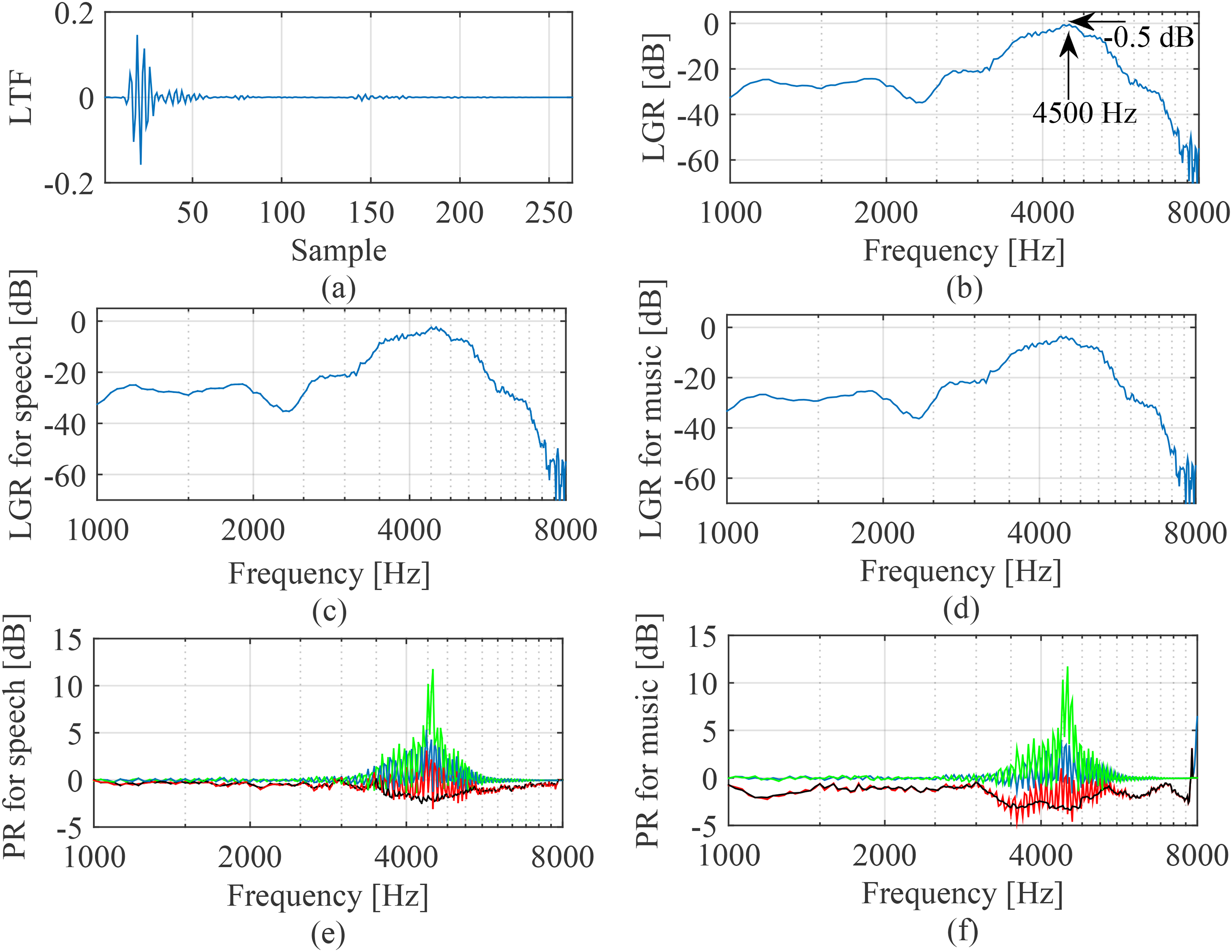
Illustration of how DeepMFC implemented feedback control when the gain margin was 0.5 dB. (a) Time-domain LTF; (b) LGR without DeepMFC; (c) LGR for speech with DeepMFC(1); (d) LGR for music with DeepMFC(3); (e) PR for speech; (f) PR for music. For (e) and (f) the PR is between: the input and output signals – black; the input and target signals – blue; the output and target signals – red. For completeness, the PR between the unprocessed signal and the target signal at the receiver is also plotted in (e) and (f) using green. LTF: loop transfer function; LGR: loop gain response; PR: power ratio.

Conclusions and Future Prospects

This paper evaluated the performance of three versions of DeepMFC in handling feedback, using both speech and music as the sources. When the source was music and the gain margin was set to 0 dB or $- 5$ dB, the distortion caused by DeepMFC(3) was appropriately characterized by HAAQI scores and could also be heard by NH listeners, resulting in lower preference scores for DeepMFC than for PEM–AFC. When the sound source was speech, DeepMFC(1) was subjectively preferred over PEM–AFC for gain margins of 0 dB and $- 5$ dB, but HASQI-V2 scores were lower for DeepMFC(1) than for PEM–AFC. This might have happened because the speech quality was relatively high and PEM–AFC contained some howling components at the beginning of an utterance. When the gain margin was set to $- 5$ dB and $- 10$ dB, the combination PEM–AFC+DeepMFC achieved the best performance for both speech and music in the subjective listening tests. Only the two speech quality metrics correctly predicted these subjective results. The HAAQI gave the highest scores for PEM–AFC. These inconsistent results indicate that HAAQI scores do not always correctly predict subjective preferences.

This paper also helped to clarify the way in which DeepMFC handles feedback. When a closed-loop system works at a marginally stable gain, DeepMFC can reduce the excess gain that occurs for frequencies where the loop gains are just below 0 dB. By comparing the PR between the input and output signals of DeepMFC, it was shown that DeepMFC suppressed the excess gain frame by frame. When a closed-loop system without feedback control worked with a gain margin of $- 4$ dB, inserting DeepMFC into the closed-loop system reduced the loop gain by up to 4 dB at the frequency that had the largest loop gain, ensuring stability and avoiding the introduction of continuous howling components. However, the excess gain problem was not completely solved by DeepMFC alone when the gain margin in decibels was negative. Because the training data set was generated only using simulated closed-loop systems working at a marginally stable gain, this problem might have been caused by the unmatched training and test conditions. Our preliminary experiments have indicated that the problem of excess gain in highly unstable systems could not be solved solely by increasing the number of parameters of the DeepMFC model or by using a more powerful deep-learning model, such as the multi-stage method (Li et al., 2021). Possibly, other more powerful deep-learning models can solve the problem of excess gain, but this is outside the scope of the present paper.

In this paper, the forward path was simplified as having a uniform linear gain, and all simulations were carried out under this condition. Although this simplified model of the forward path is commonly used in evaluating the performance of feedback control methods (Hellgren, 2002; Spriet et al., 2005; Lee et al., 2017), the frequency response of the forward path for a hearing aid is rarely uniform (Moore et al., 2010; Dillon, 2012) and often changes over time because of hearing-aid processing such as noise suppression and multichannel dynamic range compression (Moore, 1987; Kates, 2008; May et al., 2018). The influence of frequency-gain characteristics and hearing-aid processing on the performance of DeepMFC needs to be assessed. When the frequency-gain characteristics and hearing-aid processing are known in advance, their effects on the target sound at the receiver can be simulated. Better performance may be achieved when these effects are taken into account in generating the training data set for DeepMFC.

This paper evaluated the performance of DeepMFC only for speech and music sound sources. However, a hearing aid should also provide good perception of environmental sounds (Pichora-Fuller & Singh, 2006). There is a need to assess how well DeepMFC works when the hearing aid input includes a wide range of environmental sounds. Li et al. (2021) showed that for noise suppression and dereverberation tasks, speech and other types of sounds were processed appropriately when these other sounds were included as training targets in addition to speech. It will be interesting to assess whether DeepMFC can be trained to reduce the deleterious effects of acoustic feedback without introducing significant distortion for other types of sounds.

Footnotes

Acknowledgements

We thank two reviewers and the Editor-in-Chief Dr. Andrew Oxenham for very helpful and insightful comments on an earlier version of this paper.

Declaration of Conflicting Interests

The authors declared no potential conflicts of interest with respect to the research, authorship, and/or publication of this article.

Funding

The authors disclosed receipt of the following financial support for the research, authorship, and/or publication of this article: This work was supported by National Key R $&$ D Program of China (2021YFB3201702).

ORCID iDs

Chengshi Zheng

Brian C. J. Moore

Notes

References

Arehart

K. H.

Kates

J. M.

Anderson

M. C.

(2010). Effects of noise, nonlinear processing, and linear filtering on perceived speech quality. Ear and Hearing, 31(3), 420–436. https://doi.org/10.1097/AUD.0b013e3181d3d4f3

Arehart

K. H.

Kates

J. M.

Anderson

M. C.

(2011). Effects of noise, nonlinear processing, and linear filtering on perceived music quality. International Journal of Audiology, 50(3), 177–190. https://doi.org/10.3109/14992027.2010.539273

Atal

B. S.

Schroeder

M. R.

(1970). Adaptive predictive coding of speech signals. Bell System Technical Journal, 49(8), 1973–1986. https://doi.org/10.1002/j.1538-7305.1970.tb04297.x

Berdahl

Harris

(2010). Frequency shifting for acoustic howling suppression. In Proceedings of the 13th International Conference on Digital Audio Effects, Graz, Austria, 6-10 September 2010.

Bisgaard

Vlaming

M. S. M. G.

Dahlquist

(2010). Standard audiograms for the IEC 60118-15 measurement procedure. Trends in Amplification, 14(2), 113–120. https://doi.org/10.1177/1084713810379609

Brady

P. T.

(1965). A technique for investigating on–off patterns of speech. The Bell System Technical Journal, 44(1), 1–22. https://doi.org/10.1002/j.1538-7305.1965.tb04135.x

Bustamante

Worrall

Williamson

(1989). Measurement and adaptive suppression of acoustic feedback in hearing aids. In Proceedings of the IEEE International Conference on Acoustics, Speech and Signal processing (ICASSP), Glasgow, UK, 23-26 May 1989. https://doi.org/10.1109/ICASSP.1989.266855.

Byrne

Dillon

(1986). The National Acoustic Laboratories’ (NAL) new procedure for selecting the gain and frequency response of a hearing aid. Ear and Hearing, 7(4), 257–265. https://doi.org/10.1097/00003446-198608000-00007

Chasin

Hockley

N. S.

(2014). Some characteristics of amplified music through hearing aids. Hearing Research, 308, 2–12. https://doi.org/10.1016/j.heares.2013.07.003

10.

Chasin

Russo

F. A.

(2004). Hearing aids and music. Trends in Amplification, 8(2), 35–47. https://doi.org/10.1177/108471380400800202

11.

Darwin

(2009). Listening to speech in the presence of other sounds. In Moore, B. C. J., Tyler, L. K. & Marslen-Wilsen, W. D (Eds.), The perception of speech: From sound to meaning. Oxford University Press, pp. 151–169. https://doi.org/10.1098/rstb.2007.2156

12.

Défossez

Usunier

Bottou

Bach

(2019). Music source separation in the waveform domain. arXiv preprint arXiv:1911.13254.

13.

Dillon

. (2012). Hearing aids. 2nd ed. Boomerang Press.

14.

Fastl

Zwicker

(2007). Psychoacoustics: Facts and models. 3rd ed. Springer Science & Business Media. https://doi.org/10.1007/978-3-540-68888-4.

15.

Foley

(1989). Adaptive periodic noise cancellation for the control of acoustic howling. In IEE Colloquium on Adaptive Filters. London, UK, 22 March 1989.

16.

Glasberg

B. R.

Moore

B. C. J.

(1986). Auditory filter shapes in subjects with unilateral and bilateral cochlear impairments. The Journal of the Acoustical Society of America, 79(4), 1020–1033. https://doi.org/10.1121/1.393374

17.

Guo

Jensen

S. H.

Jensen

(2012). Novel acoustic feedback cancellation approaches in hearing aid applications using probe noise and probe noise enhancement. IEEE Transactions on Audio, Speech, and Language Processing, 20(9), 2549–2563. https://doi.org/10.1109/TASL.2012.2206025

18.

Guo

Jensen

S. H.

Jensen

(2013). Evaluation of state-of-the-art acoustic feedback cancellation systems for hearing aids. Journal of the Audio Engineering Society, 61(3), 125–137.

19.

Hellgren

(2002). Analysis of feedback cancellation in hearing aids with filtered-X LMS and the direct method of closed loop identification. IEEE Transactions on Speech and Audio Processing, 10(2), 119–131. https://doi.org/10.1109/89.985549

20.

Hockley

N. S.

Bahlmann

Fulton

(2012). Analog-to-digital conversion to accommodate the dynamics of live music in hearing instruments. Trends in Amplification, 16(3), 146–158. https://doi.org/10.1177/1084713812471906

21.

Loizou

P. C.

(2007). Evaluation of objective quality measures for speech enhancement. IEEE Transactions on Audio, Speech, and Language Processing, 16(1), 229–238. https://doi.org/10.1177/1084713812471906

22.

Kates

J. M.

(1991). Feedback cancellation in hearing aids: Results from a computer simulation. IEEE Transactions on Signal Processing, 39(3), 553–562. https://doi.org/10.1109/78.80875

23.

Kates

J. M.

(2008). Digital hearing aids. Plural Publishing.

24.

Kates

J. M.

Arehart

K. H.

(2014). The hearing-aid speech quality index (HASQI) version 2. Journal of the Audio Engineering Society, 62(3), 99–117. https://doi.org/10.17743/jaes.2014.0006

25.

Kates

J. M.

Arehart

K. H.

(2016). The hearing-aid audio quality index (HAAQI). IEEE/ACM Transactions on Audio, Speech, and Language Processing, 24(2), 354–365. https://doi.org/10.1109/TASLP.2015.2507858

26.

Kates

J. M.

Arehart

K. H.

(2022). An overview of the HASPI and HASQI metrics for predicting speech intelligibility and speech quality for normal hearing, hearing loss, and hearing aids. Hearing Research, 426, 108608. https://doi-10.1016/j.heares.2022.108608

27.

Kirchberger

Russo

F. A.

(2016). Dynamic range across music genres and the perception of dynamic compression in hearing-impaired listeners. Trends in Hearing, 20, 1–16. https://doi.org/10.1177/2331216516630549

28.

Lee

C. H.

Kates

J. M.

Rao

B. D.

Garudadri

(2017). Speech quality and stable gain trade-offs in adaptive feedback cancellation for hearing aids. The Journal of the Acoustical Society of America, 142(4), EL388–EL394. https://doi.org/10.1121/1.5007278

29.

Liu

Luo

Zheng

. (2021). A simultaneous denoising and dereverberation framework with target decoupling. In Proceedings of the Annual Conference of the International Speech Communication Association (INTERSPEECH), Brno, Czechia, 30 August–4 September 2021. https://doi.org/10.21437/Interspeech.2021-1137.

30.

Makhoul

(1975). Linear prediction: A tutorial review. Proceedings of the IEEE, 63(4), 561–580. https://doi.org/10.1109/PROC.1975.9792

31.

Manilow

Wichern

Seetharaman

Le Roux

(2019). Cutting music source separation some Slakh: A dataset to study the impact of training data quality and quantity. In Proceedings of the IEEE Workshop on Applications of Signal Processing to Audio and Acoustics (WASPAA), New Paltz, NY, USA, 20-23 October 2019. https://doi.org/10.1109/WASPAA.2019.8937170.

32.

May

Kowalewski

Dau

(2018). Signal-to-noise-ratio-aware dynamic range compression in hearing aids. Trends in Hearing, 22, 1–12. https://doi.org/10.1177/2331216518790903

33.

Moore

B. C. J.

(2022). Listening to music through hearing aids: Potential lessons for cochlear implants. Trends in Hearing, 26, 1–13. https://doi.org/10.1177/23312165211072969

34.

Moore

B. C. J.

(1987). Design and evaluation of a two-channel compression hearing aid. Journal of Rehabilitation Research and Development, 24(4), 181–192.

35.

Moore

B. C. J.

(2013). An introduction to the psychology of hearing. 6th ed. Brill,

36.

Moore

B. C. J.

(2016). Effects of sound-induced hearing loss and hearing aids on the perception of music. Journal of the Audio Engineering Society, 64(3), 112–123. https://doi.org/10.17743/jaes.2015.0081

37.

Moore

B. C. J.

Glasberg

B. R.

Stone

M. A.

(2010). Development of a new method for deriving initial fittings for hearing aids with multi-channel compression: CAMEQ2-HF. International Journal of Audiology, 49(3), 216–227. https://doi.org/10.3109/14992020903296746

38.

Moore

B. C. J.

Stone

M. A.

Füllgrabe

Glasberg

B. R.

Puria

(2008). Spectro-temporal characteristics of speech at high frequencies, and the potential for restoration of audibility to people with mild-to-moderate hearing loss. Ear and Hearing, 29(6), 907. https://doi.org/10.1097/AUD.0b013e31818246f6

39.

Moore

B. C. J.

Wojtczak

Vickers

D. A.

(1996). Effect of loudness recruitment on the perception of amplitude modulation. The Journal of the Acoustical Society of America, 100(1), 481–489. https://doi.org/10.1121/1.415861

40.

Naylor

P. A.

Gaubitch

N. D.

(2010). Speech dereverberation. Springer. https://doi.org/10.1007/978-1-84996-056-4.

41.

Nielsen

J. L.

Svensson

U. P.

(1999). Performance of some linear time-varying systems in control of acoustic feedback. The Journal of the Acoustical Society of America, 106(1), 240–254. https://doi.org/10.1121/1.427053

42.

Nyquist

(1932). Regeneration theory. The Bell System Technical Journal, 11(1), 126–147. https://doi.org/10.1002/j.1538-7305.1932.tb02344.x

43.

Patronis, Jr

E. T.

(1978). Electronic detection of acoustic feedback and automatic sound system gain control. Journal of the Audio Engineering Society, 26(5), 323–326.

44.

Paul

D. B.

Baker

J. M.

(1992, February 23–26). The design for the Wall Street Journal-based CSR corpus. Speech and Natural Language: Proceedings of a Workshop held at Harriman, New York.

45.

Pichora-Fuller

M. K.

Singh

(2006). Effects of age on auditory and cognitive processing: Implications for hearing aid fitting and audiologic rehabilitation. Trends in Amplification, 10(1), 29–59. https://doi.org/10.1177/108471380601000103

46.

Quatieri

T. F.

(2006). Discrete-time speech signal processing: Principles and practice. Pearson Education India.

47.

Reddy

C. K. A

Dubey

Gopal

Cutler

Braun

Gamper

Aichner

Srinivasan

(2021). ICASSP 2021 Deep Noise Suppression Challenge. In Proceedings of the IEEE International Conference on Acoustics, Speech and Signal processing (ICASSP), Toronto, ON, Canada, 06-11 June 2021. https://doi.org/10.1109/ICASSP39728.2021.9415105.

48.

Rix

Beerends

Hollier

Hekstra

(2001). Perceptual evaluation of speech quality (PESQ)-a new method for speech quality assessment of telephone networks and codecs. In Proceedings of the IEEE International Conference on Acoustics, Speech, and Signal Processing (ICASSP), Salt Lake City, UT, USA, 7-11 May 2001. https://doi.org/10.1109/ICASSP.2001.941023.

49.

Roederer

J. G.

(2009). The physics and psychophysics of music. Springer-Verlag, https://doi.org/10.1007/978-0-387-09474-8 .

50.

Rotaru

Albu

Coanda

(2012). A variable step size modified decorrelated NLMS algorithm for adaptive feedback cancellation in hearing aids. In the 10th International Symposium on Electronics and Telecommunications, Timisoara, Romania, 15-16 November 2012. https://doi.org/10.1109/ISETC.2012.6408070.

51.

Saito

Itakura

et al. (1970). A statistical method for estimation of speech spectral density and formant frequencies. Electron. Commun. Japan, A 53(1), 36–43.

52.

Schepker

Nordholm

Doclo

(2020). Acoustic feedback suppression for multi-microphone hearing devices using a soft-constrained null-steering beamformer. IEEE/ACM Transactions on Audio, Speech, and Language Processing, 28, 929–940. https://doi.org/10.1109/TASLP.2020.2975390

53.

Schroeder

M. R.

(1964). Improvement of acoustic-feedback stability by frequency shifting. The Journal of the Acoustical Society of America, 36(9), 1718–1724. https://doi.org/10.1121/1.1919270

54.

Spriet

Proudler

Moonen

Wouters

(2005). Adaptive feedback cancellation in hearing aids with linear prediction of the desired signal. IEEE Transactions on Signal Processing, 53(10), 3749–3763. https://doi.org/10.1109/TSP.2005.855108

55.

Tan

C. T.

Moore

B. C. J.

(2008). Perception of nonlinear distortion by hearing-impaired people. International Journal of Audiology, 47(5), 246–256. https://doi.org/10.1080/14992020801945493

56.

Tan

Wang

(2020). Learning complex spectral mapping with gated convolutional recurrent networks for monaural speech enhancement. IEEE/ACM Transactions on Audio, Speech, and Language Processing, 28, 380–390. https://doi.org/10.1109/TASLP.2019.2955276

57.

Torcoli

Kastner

Herre

(2021). Objective measures of perceptual audio quality reviewed: An evaluation of their application domain dependence. IEEE/ACM Transactions on Audio, Speech, and Language Processing, 29, 1530–1541. https://doi.org/10.1109/TASLP.2021.3069302

58.

Waterschoot

T. V.

Moonen

(2010). Comparative evaluation of howling detection criteria in notch-filter-based howling suppression. Journal of the Audio Engineering Society, 58(11), 923–940.

59.

Zhang

Hansen

J. H.

(2007). Analysis and classification of speech mode: whispered through shouted. In Proceedings of the Annual Conference of the International Speech Communication Association (INTERSPEECH), Antwerp, Belgium, 27-31 August 2007.

60.

Zheng

Hofmann

Kellermann

(2016). Analysis of additional stable gain by frequency shifting for acoustic feedback suppression using statistical room acoustics. IEEE Signal Processing Letters, 23(1), 159–163. https://doi.org/10.1109/LSP.2015.2507205

61.

Zheng

Wang

Moore

B. C. J.

(2022a). A deep learning solution to the marginal stability problems of acoustic feedback systems for hearing aids. The Journal of the Acoustical Society of America, 152(6), 3616–3634. https://doi.org/10.1121/10.0016589

62.

Zheng

Zhang

Liu

Luo

X. D.

Moore

B. C. J

(2022b). Sixty years of frequency-domain monaural speech enhancement: From traditional to deep learning methods. Trends in Hearing, submitted.

Evaluation of deep marginal feedback cancellation for hearing aids using speech and music

Abstract

Keywords

Introduction

Methods

DeepMFC Models

Comparison Control Approaches, Stimuli, and Procedure

Feedback Control Approaches

Stimulus Generation

Objective Quality Assessment

Subjective Quality Assessment

Results

Speech Quality for Simulated NH Listeners

Speech Quality for Simulated Hearing-Impaired Listeners

Music Quality for Simulated NH Listeners

Music Quality for Simulated Hearing-Impaired Listeners

Results of the Listening Test for Speech

Results of the Listening Test for Music

Characterization of How DeepMFC Works for Speech and Music

Conclusions and Future Prospects

Footnotes

Acknowledgements

Declaration of Conflicting Interests

Funding

ORCID iDs

Notes

References