Mechanisms of Spectrotemporal Modulation Detection for Normal- and Hearing-Impaired Listeners

Abstract

Spectrotemporal modulations (STM) are essential features of speech signals that make them intelligible. While their encoding has been widely investigated in neurophysiology, we still lack a full understanding of how STMs are processed at the behavioral level and how cochlear hearing loss impacts this processing. Here, we introduce a novel methodological framework based on psychophysical reverse correlation deployed in the modulation space to characterize the mechanisms underlying STM detection in noise. We derive perceptual filters for young normal-hearing and older hearing-impaired individuals performing a detection task of an elementary target STM (a given product of temporal and spectral modulations) embedded in other masking STMs. Analyzed with computational tools, our data show that both groups rely on a comparable linear (band-pass)–nonlinear processing cascade, which can be well accounted for by a temporal modulation filter bank model combined with cross-correlation against the target representation. Our results also suggest that the modulation mistuning observed for the hearing-impaired group results primarily from broader cochlear filters. Yet, we find idiosyncratic behaviors that cannot be captured by cochlear tuning alone, highlighting the need to consider variability originating from additional mechanisms. Overall, this integrated experimental-computational approach offers a principled way to assess suprathreshold processing distortions in each individual and could thus be used to further investigate interindividual differences in speech intelligibility.

Different listeners may return similar audiograms and yet present substantial differences in everyday tasks such as understanding speech-in-noise (SIN). This heterogeneity is observed not only for people clinically diagnosed with sensorineural hearing loss (SNHL; Moore, 2007) but also for middle-aged listeners with clinically normal audiometric thresholds and similar cognitive resources (Oberfeld & Kloeckner-Nowotny, 2016; Ruggles et al., 2012). It therefore represents an important challenge for auditory sciences. A current hypothesis is that suprathreshold auditory distortions, not accounted for by pure-tone audiometry, may have a substantial impact on SIN understanding (Lesica, 2018). These distortions remain poorly characterized despite their critical importance for better understanding SIN deficits and for designing more effective hearing devices (Lesica, 2018; Moore, 2007).

To understand how the auditory system processes complex suprathreshold signals and how distortions may emerge along its pathway, a critical step is to determine how spectrotemporal modulations (STMs) are encoded (Chi et al., 1999; Elhilali et al., 2003; Singh & Theunissen, 2003; Varnet et al., 2017; Venezia et al., 2016, 2019). Indeed, speech formants carry specific spectrotemporal energy patterns (Figure 1A), often modeled with elementary STMs termed ripples (Figure 1B; Chi et al., 1999; Elhilali et al., 2003; Mesgarani et al., 2006). Speech signals can be represented in the two-dimensional space formed by temporal and spectral dimensions, the modulation power spectrum (MPS; Elliott & Theunissen, 2009).

Figure 1.

Speech Viewed Through Ripples. A: Spectrogram of a speech sentence. Speech formants display clear spectrotemporal energy patterns referred to as spectrotemporal modulations (STMs; red box). B: Ripples constitute a first-order model of STMs: Their envelope modulation (top) is specified by their spectral modulation rate (cycl/oct, y axis) and their temporal modulation rate (Hz, x axis). An individual ripple maps to a single point in the modulation power spectrum (MPS) space (bottom).

There is now converging evidence that the human auditory system relies on MPS representations to analyze complex suprathreshold signals such as speech. Physiological studies have shown that the central auditory system exhibits specialized tuning to STMs (Hullett et al., 2016; Santoro et al., 2017), and behavioral studies have demonstrated that speech intelligibility is conveyed by STMs within specific ranges of temporal (1–10 Hz) and spectral (1–2 cycl/oct) modulations (Elliott & Theunissen, 2009; Venezia et al., 2016, 2020). Furthermore, results from modeling studies have shown that cortical auditory models or metrics such as the STM index, all based on decomposition of auditory signals through an STM filter bank, provide accurate accounts of SIN intelligibility scores (Bernstein et al., 2013b; Chi et al., 1999; Elhilali et al., 2003). These studies all suggest that STMs (or ripples) constitute an ideal model to probe suprathreshold auditory processing as it is actually recruited by natural speech. However, most psychoacoustical work on suprathreshold auditory processing has investigated temporal and spectral dimensions separately (as pointed out in Archer-Boyd et al., 2018; Miller et al., 2018) using, on one hand, signals with temporal-only modulations (amplitude-modulated tones or noises) or, on the other hand, frequency-modulated (FM) tones or broadband signals with spectral-only modulations, that is, spectral ripples (Bacon & Grantham, 1989; Dau et al., 1997; Eddins & Bero, 2007; Ewert et al., 2002; Houtgast, 1989; Joosten et al., 2016; Moore & Sek, 1996; Ozmera et al., 2018; Saoji & Eddins, 2007; Wallaert et al., 2018). The extent to which these results reflect the actual processing of joint spectral and temporal modulations remains to be determined.

Recently, by measuring psychoacoustical masking patterns for the detection of a target STM embedded in other masking STMs, Oetjen and Verhey (2015, 2017) provided the first direct evidence of behavioral tuning in MPS space, in the form of band-pass STM filters finely tuned to the spectral and temporal modulations of the target STM. Their results also revealed that these filters are partially directional, namely that they are not equally tuned to downward-moving ripples compared with upward-moving ripples (corresponding to the target STM). The observed filter asymmetry between negative and positive quadrants ¹ of MPS space suggests that a cascade of separable spectral and temporal filters may only provide an incomplete account of the human measurements. However, because those measurements were made using narrow-band modulation maskers, they might not fully reflect the overall processing strategy engaged by listeners to detect a target STM in broadband noise spanning a larger region of MPS space. This is the case, for instance, when phonemes must be extracted from cocktail-party noise. Such operations may require more complex integration schemes and involve specific nonlinear decision strategies. Furthermore, because these data were obtained solely with normal-hearing (NH) listeners, it remains unknown whether hearing-impaired (HI) listeners suffering from SNHL, who must cope with distorted representation of incoming signals resulting from poorer cochlear frequency analysis, exhibit similar modulation filtering characteristics (tuning, directionality).

Previous studies of STM processing in HI listeners (Bernstein et al., 2013a, 2013b, 2016; Mehraei et al., 2014; Miller et al., 2018) have demonstrated that their ability to detect STMs with specific spectral and temporal modulation rates (threshold modulation depth for detecting STM compared with nonmodulated noise) can account for a significant proportion of their variance in speech-reception thresholds in noise, beyond that accounted for by the audiogram alone. However, as pointed out by the authors (see Miller et al., 2018), several distinct mechanisms might be conflated by these measurements: broader cochlear filters due to hearing loss as well as deficits related to other processes (that were not engaged with pure tones), such as temporal fine structure (TFS) processing. In relation to the former aspect, some recent studies go as far as suggesting that upward/downward STM discrimination thresholds could serve as a proxy measure for auditory filter bandwidth (BW; Narne et al., 2019, 2020). In addition, it is important to note that these studies have examined factors that limit the ability of HI listeners to detect modulations at threshold, but these factors may differ from those recruited when extracting suprathreshold STMs from modulation noise, such as in the context of Oetjen and Verhey’s (2015) masking paradigm. Lastly, a recent study by Venezia et al. (2019), who used a data-driven approach to assess the regions of the MPS contributing to speech intelligibility for both NH and HI listeners, demonstrated that while both groups relied equally on the same regions, HI listeners use more variable filtering strategies (i.e., evidence for increased internal noise) and that this variability correlates with their degree of hearing loss.

Altogether these results suggest that to detect STM applied to noise carriers, HI listeners likely exhibit different perceptual tuning characteristics compared with NH listeners, caused by a combination of mechanisms ranging from peripheral (e.g., broadening of cochlear filters) to more central (e.g., impaired modulation tuning) as well as decisional aspects (e.g., signals could be represented with lower fidelity at readout, leading to increased internal noise). Yet, their respective role and contribution remain unclear. Thus, our main concern here is to adopt a measurement framework carrying the potential for further mechanistic insights into NH and HI listening strategies, as well as differences between the two.

In this study, we adopt a psychophysical reverse-correlation approach (Ahumada & Lovell, 1971; Murray, 2011) that obviates the limitations mentioned earlier. First, the reverse-correlation approach supports more detailed characterization than traditional masking paradigms: The latter assess the effects of single-component noise sources on perceptual filtering (Oetjen & Verhey, 2015), while the former involves a multicomponent noise source such that the different contribution of the various components can be assessed simultaneously, along with their potential interactions. Second, even though the perceptual filters returned by this method encompass all filtering stages from signal to decision, computational tools from system identification can be used to dissect the different components (Murray, 2011). More specifically, in a task where listeners must identify which of two noisy stimuli contains a target, a mismatch between perceptual filters derived separately from stimuli that contain the target (target-present) and those that do not contain the target (target-absent) can expose the presence of a nonlinear process, prompting detailed computational inspection to tease apart the contribution of filtering elements and nonlinear distortions to the overall perceptual filter. This level of inspection has refined our understanding of the nonlinear processes engaged by basic auditory tasks such as tone-in-noise detection (Joosten & Neri, 2012) and amplitude-modulation (AM) detection (Joosten et al., 2016), which had remained difficult to observe otherwise (e.g., Shub & Richards, 2009). Finally, because the method relies on the introduction of random external noise perturbations, it naturally accommodates standard double-pass techniques for the estimation of internal noise (Burgess & Colborne, 1988; Neri, 2010a).

Yet, the full potential of a reverse-correlation approach can be achieved only if two important interrelated factors are met: (a) The nature and structure of the perturbing noise source must efficiently interfere with the mechanisms engaged by listeners for detecting the target, and (b) a large data mass (several thousand trials) is necessary to derive a stable, accurate image of those mechanisms. The specific data mass required to obtain a stable perceptual filter varies with several factors, including stimulus complexity and the characteristics of the perceptual process under investigation. For example, the number of trials required to obtain an interpretable image of the perceptual filters underlying tone-in-noise detection can be as large as 10,000 when noisy perturbations are applied to the full time-frequency domain (e.g., Joosten et al., 2012; Shub & Richards, 2009). Based on these considerations, we decided to deploy the reverse-correlation approach directly in MPS space to assess the perceptual filtering processes underlying STM detection.

We considered a target STM with parameters comparable to Oetjen and Verhey (2015, 2017; temporal modulation rate: ±7.1 Hz; spectral modulation rate: 1 cycl/oct), and we designed an efficient ² low-dimensional broadband modulation masker, with components corresponding to 15° rotations of the target STM in spectrotemporal space (see Figure 2A and the Materials and Methods section). This noise can thus be represented with only 12 components spanning a so-called orientation axis in MPS space, in a manner analogous to the orientation noise used in vision (Neri, 2014a, 2015; Ringach, 1998). The corresponding spectral-temporal modulation rates make this noise particularly suited to our purpose: It is broadband in the sense that it targets different portions of the modulation filters involved in both positive and negative quadrants of MPS space (Oetjen & Verhey, 2015, 2017), and importantly these regions are critical for speech intelligibility (Elliott & Theunissen, 2009; Venezia et al., 2016, 2019).

Figure 2.

From Noisy Ripples to Perceptual Filters. A: Procedure for generating 1-D orientation noise from target STM (red dot). We create 12 different components from 15° rotations in spectrotemporal space (orange dots), thus defining a specific orientation axis (in dark blue). Each rotation corresponds to an STM with a different pairing of temporal (from –10 to 10 Hz) and spectral (from 0 to 1.4 cycl/oct) modulation rates. Orientation noise is then generated by summing these components with random amplitude and phase. B: One trial of the STM detection task. The 12 levels specifying each noise sample of the target-absent stimulus (right) are drawn from a Gaussian distribution (only 5 are shown). The target-present stimulus is generated using the same procedure, except a constant level offset is added to the component corresponding to the target orientation (left panel, red offset); note that this component always takes the same phase as the target, while the phases of the remaining components are randomly drawn. Listeners are presented with both stimuli in random order and must determine which interval contained the target-present stimulus (bottom). Here, the procedure is illustrated for an upward target, but we also tested (in different observers) detection of a downward target. C: Perceptual filters are computed by summing/subtracting the 12-component noise traces, separately classified depending on whether they contain the target or not, and on whether the listener responds correctly or incorrectly (see the Reverse-Correlation Analysis section). The resulting filters (target-absent, blue; target-present, red; all stimuli pooled together, black) are shown here as cartoon examples.

The design of orientation noise in the MPS domain was further motivated by prior experience regarding the characterization of visual processes selective for orientation (Neri, 2014a; Ringach, 1998), which becomes comparable to our problem if we consider time-frequency auditory coordinates analogous to space-space visual coordinates. In particular, these studies showed that (a) visual operators can be successfully characterized as oriented sensors (Adelson & Bergen, 1991), where orientation is defined, for example, across space-space (Neri, 2015) or space-time (Burr et al., 1986; Neri, 2014b) and that (b) using noise structured around the dimensions along which the perceptual process operates carries the potential to expose computational characteristics (e.g., gain control) that do not necessarily become measurable using other types of noise (Neri, 2015, 2018b).

In sum, the goal of the present study is to characterize the perceptual machinery underlying STM detection in noise for both NH and HI listeners using a novel reverse-correlation framework developed in the modulation domain (see earlier). The richness of the perceptual filters returned by our measurements is exploited using two types of modeling tools. We first adopt a system identification approach to assess the nonlinear characteristics of the decision process engaged in the task. This identification allows us to constrain a functional auditory model, which is subsequently used to infer the origins of the differences observed between the perceptual filters of NH and HI listeners. In particular, we rely on the (temporal) modulation filter bank (MFB) model (Dau et al., 1997), a widely used approach for simulating suprathreshold processing in the auditory system (Biberger & Ewert, 2016). The use of this multistage cascade model allowed us to test the extent to which STM processing in HI individuals can be accounted for by poorer frequency resolution at the periphery alone, or whether our results point toward a potential contribution of other mechanisms (which could originate either from peripheral or central sources; see the Discussion section).

Materials and Methods

Participants

We tested 10 NH participants (age range 21–37 years; M = 27, standard deviation [SD] = 5) with audiometric thresholds ≤ 25 dB HL in the 250–8000 Hz range in both ears and 7 HI participants with similar mild to moderate symmetrical flat SNHL (age range 59–67 years; M = 63, SD = 3). Their audiograms, demographic characteristics, and corresponding experimental conditions are detailed in Figure S1 and Table S1. All subjects were naïve to the goals of the study. They gave their informed written consent prior to the experiment in compliance with the Declaration of Helsinki and were paid for their participation.

Stimuli

Ripple or orientation noise was constructed by summing 12 elementary ripples of different spectral/temporal modulation rates with different energy/phases (see Figure 2A and B). Spectral/temporal modulation rate values were selected so that the envelopes of the 12 ripple components corresponded to rotations of 15° around a target signal with temporal modulation rate of 7.1 Hz and spectral modulation rate of 1 cycl/oct. In our plots, the target orientation is assigned a value of 0 (see labels arranged along orientation axes in Figure 2A and B). If we denote the envelope of each component at full modulation depth with notation M_j where index j ranges between 1 and 12, j = 7 indicates the component corresponding to the target. For each stimulus, the level of each component is denoted by k_j and was randomly drawn from a normal distribution (SD = 3 dB, restricted to ±3 SD), while the phase of each component was assigned a pseudorandom value chosen from [0, pi/4, pi/2, or 3 pi/4] (except for the component aligned with the target, the phase of which always matched the phase randomly drawn for the target). These masking STMs constitute the source of external noise considered in the present study, meaning that the external noise SD was equal to 3 dB. The 12 envelopes were superimposed to generate a composite noise envelope N = ∑_j k_jM_j (an example is shown in Figure 2B). We similarly constructed a signal envelope T by setting all k values to 0 except for k₇=ρ (amplitude of target component). The noise-only envelope N (target-absent stimulus), the signal-only envelope T (reminder stimulus), and the signal+noise envelope T + N (target-present stimulus) were smoothly tapered around the edges by a rounded-square mask to occupy a time-frequency region of 250 ms/600–3400 Hz, and were then applied to pink-like noise carriers made of 400 log-spaced sinusoidal frequency components with random phases spanning the 250–8000 Hz frequency region. A new carrier was generated for every stimulus. If we denote the smoothing window with S and a given carrier sample with C, this procedure simply amounts to (T + N)xSxC (for the target-present stimulus) where x is element-by-element multiplication (examples are shown in Figure 2B). We emphasize that, in the expression just detailed, the signal is added at the level of the modulation envelope before applying the carrier. Each sample of ripple noise is represented by the 12-component vector n_i^[q,z]: the vector sample presented on trial i in the target-absent (q = 0) or target-present interval (q = 1) that was classified by the listener as containing the target (z = 1) or not (z = 0). For example, n₉^[1,0] is the noise sample that was added to the target signal on the ninth trial, which the observer classified as not containing the target.

Procedure

We used a two-interval-forced-choice design: On each trial, listeners were presented with both target-absent and target-present stimuli in temporal succession (but randomly ordered) and were asked to indicate which interval contained the target-present stimulus. Stimulus duration was 250 ms; interstimulus interval was 350 ms. A different sample of ripple noise (aforementioned k values) was applied to the two intervals and on every new trial. The offset value applied to the target component (aforementioned ρ value) was adjusted on a listener-by-listener basis through preliminary experiments measuring the value associated with stable performance of d′ ∼ 1 (Murray, 2011). It was then kept constant for each listener throughout the rest of the experiment. The direction of the target signal (upward or downward) was randomly varied between subjects (see Table S1 for details) to verify that our conclusions remain unaffected by target direction. All stimuli were level-normalized and presented at 75 dB sound pressure level. Physical level was therefore identical between NH and HI individuals and ensured that all frequency components were audible to HI individuals.

Sounds were generated at a sampling rate of 44.1 kHz and converted via a 16-bit resolution Meridian Explorer2 sound card. They were presented monaurally to the best ear through headphones (Beyerdynamic DT 770 pro 250 ohms). Sound level was calibrated using a Bruel & Kjaer artificial ear (Type 4153, IEC318). Participants were tested individually using identical equipment (laptop, soundcard, headphones) but at two different sites: NH individuals were tested inside a double-walled sound-insulated booth in the laboratory (in Paris, FR); HI individuals were tested in a clinical environment equipped with laboratory facilities (in Reims, FR). HI individuals were not tested inside sound-insulated booths; however, the average environmental noise level was low, and other individuals were not allowed into the testing room during the experiments.

The experiment was divided into six test sessions. In the first session, auditory thresholds (125–8000 Hz) were measured in quiet for both ears using a Bekesy tracking procedure. Instructions were then given to the participants who were familiarized with the STM detection task. Task difficulty was progressively increased by reducing the target offset level (ρ) while monitoring performance over training blocks of 100 trials, until sensitivity decreased to about d′∼1 and remained stable. The associated target offset was then kept constant for the following five sessions.

Responses were entered via keyboard, and participants received audiovisual feedback after each trial (green text + two-tone consonant chord for correct vs. red text + two-tone dissonant chord for incorrect responses). Each of these five sessions comprised a first training block of 25 trials (not used for analysis) followed by 11 blocks of 100 trials. To aid participants in maintaining a stable memory representation of the target signal and to sustain their attentional level, we presented four repetitions of a signal-only stimulus (envelope T detailed previously), one every 25 trials. All stimuli presented across the 11 blocks were different, except for one block (randomly chosen) that was repeated twice (at a random position in the session) to evaluate the percentage of agreement between the two passes for the purpose of computing internal noise intensity (Burgess & Colborne, 1988; Green, 1964; Neri, 2010a).

NH listeners completed each session in approximately 60–85 min; sessions were separated by a minimum of 5 hr. The schedule of the experiment was slightly different for HI listeners due to time constraints at the clinic. Depending on the participant, there were between 4 and 5 slots of 90–120 min of data collection (participants were allowed as many pauses as they wished) scheduled on different days, where they could start/stop at any time during a given session and start from where they left during the following session. A total of about ∼5k trials were collected for each participant in the main task (see Table S1 for details).

Assessment of Internal Noise

We follow here the signal-detection theory (SDT) framework. Within this framework, listeners reach their decision as to which interval contains the target by evaluating, for each interval, a ‘decision variable’; their ability to detect the target is therefore limited by the amount of variability associated with this variable. The extent of said variability is determined by two factors: (a) systematic properties of the system that filter out different components of external noise to extract the target signal (which we assess using reverse correlation, see below) and (b) nonsystematic random variations of the system, called internal noise, that are decoupled from external noise properties. Internal noise thus refers to the cumulative contribution of all potential sources of variability within the system, from periphery to central and decisional levels (e.g., stochasticity of neuronal firing, attentional fluctuations; Faisal et al., 2008). Both factors cause trial-to-trial fluctuations of the decision variable; in classical implementations of SDT, the variance of the decision variable is therefore modeled as the sum of the two variances associated with these two factors (Green & Swets, 1966). Because the decision variable is a unit-less quantity, the variance due to internal noise is defined as a fraction of the variance due to external noise (Burgess & Colborne, 1988; Neri, 2010a). We measure the square root of this quantity (ratio of SDs rather than variances) via the established double-pass technique (Burgess & Colborne, 1988; Neri, 2010a): In this approach, the internal-to-external noise ratio is inferred from an SDT model fitted to the percentage of correct responses and percentage of agreement (i.e., same responses) measured across repeated presentation of the same trials (see previous studies for a detailed description of this model, e.g., Joosten & Neri, 2012). Internal noise values were obtained for each individual from the repetition of ∼500 trials (exact trial counts are reported in Table S1).

Reverse-Correlation Analysis

We use reverse correlation to derive perceptual filters engaged by listeners in our task (Murray, 2011). To assess the presence of potential nonlinear processes, filters are derived from each individual separately for target-absent and target-present stimuli. It has been analytically demonstrated that, if listeners behave linearly (i.e., template-matching model), target-absent and target-present perceptual filters must be identical (Ahumada, 2002; Murray, 2011). Any departure from this prediction indicates the presence of nonlinear strategies (above and beyond the final nonlinear decision rule that generates the psychophysical response), prompting (a) the use of computational tools to decipher the type of nonlinearity involved (Joosten et al., 2016) and (b) reliance on target-absent filters to interpret underlying weighting strategies because target-absent estimates are minimally contaminated by distortions produced by the interaction between the nonlinearity and the energy increment at target orientation (see Neri, 2010c). An early example of the distinction between target-absent and target-present perceptual filters in the auditory literature is the study by Ahumada and Lovell (1971), who showed that frequency weighting profiles for tone detection in noise differ between target-absent and target-present stimuli. The authors suggested that this difference reflects a nonlinear rule for combining features potentially signaling the target. Another more recent example is Joosten and Neri (2012), who derived time-frequency filters underlying detection of a brief tone embedded in noise. They observed that the time-frequency structure of target-absent filters was much coarser than corresponding estimates from target-present stimuli; this result can be accounted for by a nonlinear MAX operation to read out the information available from the bank of frequency channels (see Joosten & Neri, 2012). Using the notation introduced earlier and in keeping with current literature (Murray, 2011), the target-absent perceptual filter was computed as p^[0]= avg(n_i^[0,1]) - avg(n_i^[0,0]), while the target-present filter was computed as p^[1]=avg(n_i^[1,1])-avg(n_i^[1,0]), where avg() indicates averaging across all stimuli of the indexed type. The full (i.e., aggregate) perceptual filter is simply p = p^[1]+p^[0] and returns an image of the overall process engaged by listeners. All p estimates are normalized by σ_ext, the SD of the external noise source. A schematic illustration is provided in Figure 2C.

Statistical Analyses

We used nonparametric statistics to compare the distributions of indexes derived from our measurements either against 0 or between two samples (Wilcoxon signed-rank and rank-sum tests) and explore potential correlations (Spearman rho). Due to the limited number of subjects within each group, we also used bootstrap methods (Efron & Tibshirani, 1994) to assess the robustness of our observations at the group level, which were first inferred from the averaged data (bootstrap was conducted to build, for example, 10,000 new samples of n subjects from the initial pool of n subjects, so we could compute the indexes from the data of these new samples).

Filters Derived From the MFB Model

We compare perceptual filters derived from human data with those simulated from a simplified version of the temporal MFB model (Dau et al., 1997); this version corresponds to one introduced by prior studies (Cabrera et al., 2019; King et al., 2019; Wallaert et al., 2018). We briefly describe the different stages of the model and the choice of parameters for our study below (see Figure 6A for an illustration of the corresponding processing cascade).

First, the input auditory stimulus is passed through a linear Gammatone filter bank as implemented in Hohmann (2002) covering the frequency range of our stimuli (620–3300 Hz; filter density used was 1/equivalent rectangular bandwidth [ERB], but we verified that this choice was not limiting and that higher density values lead to similar results). Second, the envelope of each channel is extracted through Hilbert transform, without any compressive stage (not necessary for the present case that compares time series) and low-pass filtered (cutoff frequency of 1500 Hz) to simulate hair-cell transduction and adaptation. Third, signals from each channel are passed through a MFB (consisting of five first-order Butterworth filters log-spaced between 0.5 and 20 Hz) with a Q value of 1 (consistent with experimental data showing that this parameter is similar in NH and HI listeners; Sek et al., 2015). Fourth, the phase in low (<5 Hz) modulation channels was discarded by replacing signals at the output of these modulation filters with their Hilbert envelopes, to account for the upper limit of modulation phase sensitivity (Dau, 1996; Sheft & Yost, 2007). The resulting ‘venelopes’ (envelopes of envelopes; Ewert et al., 2002) are scaled so as to preserve their original root-mean-square value. Finally, the representations are temporally downsampled by a factor of 10. The final internal representation of a given signal thus spans three axes (time × frequency × modulation). A nonlinear operation produces the final decision: To decide between two stimuli where one contains the target, the model compares each stimulus representation with the stored representation for the target via normalized cross-correlation for each frequency channel and each modulation channel. The correlation functions are summed across bands to estimate the time lag corresponding to the best match. The model finally selects the stimulus producing the highest correlation value.

We simulate perceptual filters from the model for two target directions (either upward or downward) and for different cochlear BWs ranging between 0.5-ERB and 4-ERB to explore the effect of frequency selectivity on the estimated filters. These filters are derived from the simulated binary responses using reverse correlation in the same way as described previously for human listeners. Each combination of target direction and cochlear BW was tested using a different set of 20,000 trials constructed exactly as the ones presented to the participants in the task. The signal-to-noise ratio (SNR) of these stimuli (i.e., level of offset at target orientation subtracted by the mean level of the components at other orientations, divided by the external noise SD) was similar to the one used on average with NH participants (3.3 dB), because the simulated sensitivity was within human range (d′∼1). The stored target representation was constructed by subtracting the internal representation of a ripple stimulus containing only the target component either upward (to derive filters for the upward target) or downward (to derive filters for the downward target) from the internal representation of a noise stimulus consisting of the same carrier without imposed modulations. This is a standard procedure for constructing an exemplar that primarily reflects the modulations of the target component but not the intrinsic modulations related to the fine structure of the carrier (Dau et al., 1996; King et al., 2019). A new internal representation was generated every block of 50 trials, specified by target direction (upward or downward) and random phase (among the 4 possible values). Following the steps outlined earlier, estimates obtained for the two target directions and the four different phase values of the template were pooled together, because we did not observe systematic differences (consistent with the observed lack of such differences from human estimates).

Results

Before detailing our results, we draw attention to the fact that all listeners tested in this experiment were able to successfully perform the detection task: We individually tailored target intensity to reach a performance of d′∼1 (76% correct responses). In presenting our results, we pooled data from all experimental sessions because we observed little learning/retuning effects over time for both groups (see complementary analysis in SI 2). We also pooled data across different target phases, because we found no differences in filter estimates computed separately for the four possible phase values.

Similar Level of Internal Noise for NH and HI Individuals in a Comparable Performance Regime

We measure three factors that primarily govern psychophysical performance: stimulus discriminability/sensitivity (d′), response bias, and internal noise intensity; we find no substantial difference between NH and HI groups (Figure S2). There is no response bias (target-unrelated preference for one interval) in either group (NH group: c = 0.1, SD = 0.2; HI group: c = 0.0, SD = 0.2; p = .31). Sensitivity values are comparable between groups (NH group: d′ = 0.7, SD = 0.2; HI group: d′ = 1.1, SD = 0.6; p = .04), and internal noise (assessed using double-pass consistency; see the Materials and Methods section) is similar between NH (M = 1.3, SD = 0.4) and HI individuals (M = 1.3, SD = 0.5; p = .96). We report no correlation between internal noise and d′ values (NH: p = .51; HI: p = .44), indicating that these two metrics reflect different aspects of perceptual processing in our task (Figure S2). Finally, we consider absolute efficiency (defined as the squared ratio between measured and ideal d′ values; Green & Swets, 1966; Tanner & Birdsall, 1958) to compare the empirical results with those produced by an ideal observer. Complementary analyses show that internal noise values correlate negatively with both absolute efficiency and the target-specific energy returned by perceptual filters (see SI 1); this result, which is consistent with theoretical considerations, confirms that internal noise values from the double-pass protocol can be interpreted as meaningful estimates of internal variability associated with the detection mechanism.

Different Perceptual Filtering Between NH and HI Groups and Distinct Filters for Target-Absent and Target-Present Stimuli

We derive perceptual filters from all noise fields (black traces in Figure 3A), as well as separately from target-absent (blue) and target-present (red) stimuli (see the Materials and Methods section). Because we did not observe substantial differences between filters derived from participants who were asked to detect an upward-directed target as opposed to a downward-directed target, when averaging across observers we realign data from the two conditions so that target orientation always takes a notional value of 0 (center of x axis in Figure 3A).

Figure 3.

Perceptual Filters Change Shape Under Hearing Impairment. A: Perceptual filters derived from reverse correlation using target-absent/target-present/all noise samples (blue/red/black traces). Filters are plotted against the 1-D orientation axis (see Figure 2) and centered on target orientation (red arrow, 0°). Both average (main panels) and individual filters (side columns) are presented for each group (NH on the left, HI on the right). Shaded areas show SEM across individuals in main panels, or SD estimated by bootstrapping for individual traces. B: Distribution of two scalar metrics computed from perceptual filters showing differences between NH (green) and HI (pink) individuals. The upper panel is a measure of target-specific selectivity associated with perceptual filters (log-ratio between energy at target orientation/energy at other orientations). Lower panel shows metric designed to capture interindividual variability within each group (Pearson correlation between each individual filter and filters from every other individual within the same group). Stars show significant differences between NH and HI individuals (two-sided Wilcoxon rank-sum tests; * indicates p < . 05, *** indicates p < . 001).

Perceptual filters indicate how listeners differentially weight energy from different components when performing the task. A positive value indicates that more energy on this component steered listeners toward reporting that the target was present, while less energy on this component makes listeners less likely to identify the stimulus as containing the target. This convention applies to both target-absent and target-present perceptual filters.

We first note that, for almost every individual tested, the aggregate perceptual filter displays significant structure (no flat patterns), clearly demonstrating that our approach is capable of exposing an image/signature of the perceptual process used to detect the target STM in noise. The only exception is HI7 who returns a nearly flat pattern (bottom trace in HI filters). Because this participant produced exceptionally poor performance during the first session when his threshold level was established for subsequent data collection, all data from this participant was collected for a stimulus SNR that was 6 dB higher than other HI individuals. During the following sessions, however, his performance improved to d′ >2, a performance regime that is suboptimal for recovering accurate estimates from reverse correlation (Murray, 2011). Indeed, for this particular individual, the selected SNR level was too high for the external noise source to produce measurable impact on his behavior. Due to the intensive nature of data collection in these experiments, we were only able to test a limited number of individuals and are therefore not in a position to exclude data from this individual. However, we have verified that our conclusions remain unaffected when this individual is excluded. For similar reasons (small size of population samples), and in light of potential interindividual differences particularly within the HI group, we present and discuss relevant effects not only at group level but also at the individual-listener level.

On average and for both groups (black traces in Figure 3), the aggregate perceptual filters display the expected ‘Mexican hat’-shaped tuning profiles: a central positive peak corresponding to the orientation of the target component, flanked by negative troughs on both sides. This shape is consistent with orientation-tuning measurements from visual tasks (Neri, 2015; Ringach, 1998). The aggregate filter from HI participants (Figure 3A right) is overall reduced in amplitude compared with the corresponding measurement from NH listeners (Figure 3A left). When considering individual patterns, we observe clear deviations from the average Mexican hat shape (see Figure 3A, stacked traces on left and right sides). In the NH group, all 10 individuals produce profiles peaking at target orientation (left insets in Figure 3A), while in the HI group, some individuals produce filters peaking at orientations corresponding to higher temporal modulations and lower spectral modulations (right insets in Figure 3A). These group differences are quantitatively supported by two scalar metrics (plotted in Figure 3B) introduced to capture differences between aggregate filters from the two groups. The first metric is designed to assess the selectivity of listeners’ strategies by estimating the optimality of their perceptual filter for the assigned task: It is computed as the log-ratio between the energy of the perceptual filter at target orientation and energy at other orientations. We find greater filter selectivity for NH individuals than HI individuals (p = .02). The second metric is designed to assess interindividual variability: It is the correlation between each individual filter and filters from other individuals of that group. We find a significantly higher variability in the HI group compared with the NH group (p < .001).

Beyond these notable differences in aggregate filters, our data exhibit evident mismatch between target-present and target-absent filters for both groups: Target-present estimates contain a clear modulation around target orientation that is markedly reduced in target-absent counterparts. This result is incompatible with a linear template-matching strategy (Ahumada, 1967; Neri, 2004), prompting us to adopt computational tools that can accommodate departures from this strategy (Neri, 2010c).

Unbiased Inspection of Target-Absent Filters to Bypass Nonlinear Processes

To clarify the earlier statements, we ran simulations to assess the ability of two competing cascade computational models, a linear and a nonlinear model, to account for our filter estimates (Figure 4). Both models rely on the same structure and only differ in their final decisional stage. On each trial, these models first apply a weighting function to the 12 components of the two input stimuli s₁ and s₂ (as specified by colored 12-vector templates; Figure 4A), then either compute the sum (linear) or the maximum (nonlinear) from these traces, and finally select the stimulus producing the larger value. Here, we used different templates to best account for filters of NH and HI groups (green and magenta curves in Figure 4A). The filters (i.e., kernels) derived from these models (Figure 4B) clearly show that only the nonlinear model captures all main features of our measurements and in particular produces distinct target-present and target-absent filters. It is important to note that, while the choice of templates is arbitrary, the simulated difference between target-absent and target-present filters is not a consequence of this choice and is instead produced by the MAX nonlinearity.

Figure 4.

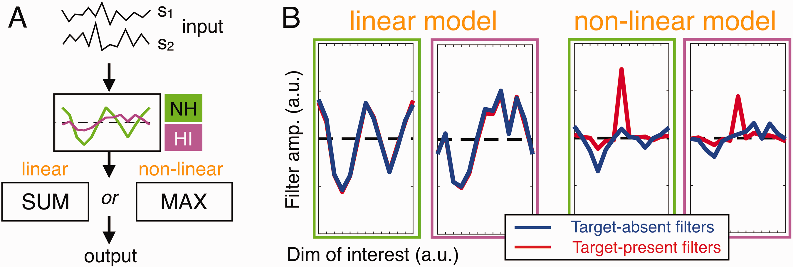
Nonlinear Strategies Are Reflected by Mismatched Target-Present and Target-Absent Filters. A: Structure of the two cascade models tested here. They rely on the same weighting profiles (green/magenta templates for NH/HI) but differ in their final decision stage (linear: sum; nonlinear: max). B: Simulated filters (same plotting conventions as Figure 3) show that only the nonlinear model can account for our data.

These computational simulations show that a simple variant of the popular MAX uncertainty model (Pelli, 1985) can account for important aspects of our experimental estimates (see also Dau et al., 1997; Joosten & Neri, 2012). This result means that the perceptual strategy engaged by both NH and HI participants was strongly nonlinear, prompting us to focus our analyses on target-absent filters (Neri, 2018b): As expected from theory (Neri, 2004, 2010b; Tjan & Nandy, 2006) and as illustrated via our simulations (Figure 4), target-absent filters closely resemble the model weighting curves preceding the nonlinear stage (compare blue profiles in Figure 4B with model weighting functions in Figure 4A). These estimates therefore provide a more transparent view of the weighting strategy adopted by human listeners (see below).

In the NH group, target-absent filters present a peak at target orientation; in the HI group, the peak is shifted toward lower spectral modulation and higher temporal modulation rates. In both groups, target-absent filters display approximate symmetry around the pure temporal modulations line (symmetry of horizontal traces in Figure 5). To aid visualization of this result, we project target-absent perceptual filters onto spectral-temporal dimensions and reconstruct their shape across both quadrants of MPS space (see Figure 5) under the assumption of spectral/temporal separability (Chi et al., 1999; Venezia et al., 2019). Overall and in both groups, filters are symmetric between negative and positive quadrants of MPS space, except for slightly higher values within the quadrant containing the target (which we arbitrarily project on the left side for all subjects; see contour plots in Figure 5). In the NH group, nondirectional band-pass characteristics are finely tuned to the parameters of the target modulation (peaks in Figure 5 [left] fall near target location). In the HI group, the frequency characteristics are biased toward lower spectral modulation rate and higher temporal modulation rate (peaks in Figure 5 [right] are closer to bottom corners).

Figure 5.

Hearing Impairment Shifts Weighting Strategy Toward Lower Spectral Rates. Empirical perceptual filters derived from target-absent stimuli are projected along the two dimensions of native modulation space, that is, temporal and spectral modulation (see horizontal and vertical traces; shaded regions show SEM across polynomial-fitted curves for each individual). Separate projections (superimposed vertically) were derived from data points in the negative versus positive quadrant of MPS space (leftward vs. rightward-pointing arrows); these traces are barely distinguishable. To obtain a more readable image of the underlying strategies, we reconstruct full filters in both quadrants of MPS space by multiplying the corresponding traces (thus assuming quadrant separability). Red arrows point to target modulation (–7.1 Hz; 1 cycl/oct), which we arbitrarily projected on the left quadrant for all listeners (i.e., also for those with a downward target). For the NH group (left), the filter displays band-pass characteristics well aligned with the target modulation; for the HI group (right), filter peak is shifted toward lower spectral modulation rate and higher temporal modulation rate.

To summarize the aforementioned results, the perceptual strategy of both NH and HI groups could be modeled as largely nondirectional band-pass filters followed by a nonlinear rule akin to a MAX operation. The frequency characteristics of the band-pass filters match those specified by the target STM in the NH group, but not in the HI group. In the latter, they are shifted toward lower spectral modulation and higher temporal modulation rate values. While this computational analysis clarifies the nonlinear decision strategy adopted by listeners, the MAX model is not intended as a physiological implementation of known facts about the auditory system; it is used here to provide an overall description of the perceptual process engaged in the task. In particular, the band-pass weighting images inferred from target-absent filters (Figure 5) reflect all auditory processing stages (from periphery to central levels); therefore, the observed differences between the two groups cannot be directly related to specific stages. This level of inspection requires the use of a biologically inspired model, where specific stages can be related to their physiological counterparts.

Filters Predicted by the MFB Model

To further understand the potential origin of the deficits that may underlie the observed differences between NH and HI listeners, we resort to a simplified version (see the Materials and Methods section) of the popular MFB model (Dau et al., 1997). Guided by the aforementioned computational results, we are in a position to make informed choices regarding the final decisional stage of the model: We model this stage around the maximum value returned by a cross-correlation device (Figure 6A, see the Materials and Methods section for further details), in line with previous studies (Cabrera et al., 2019; King et al., 2019; Wallaert et al., 2018). To gain some insight into how SNHL contributes to the differences observed in the HI group, we explored the effect of frequency selectivity—one particular deficit associated with SNHL (Lesica, 2018; Moore, 2007)—on the simulated filters. More specifically, we varied filter BW at the cochlear stage between 0.5-ERB and 4-ERB wide (see the Materials and Methods section for details).

Figure 6.

Broadening of Cochlear Filters Explains Some, but Not All, Impairment-Specific Effects. A: Structure of the modulation filter bank model (cochlear filters are highlighted in orange). B: Examples of filters derived from reverse-correlation analysis of the model’s predictions using gamma-tone filters with bandwidths (BW) 1, 2, and 3 ERBs. C: Correlation between model and group-based target-absent filters for various BWs (0.5–4 ERBs), indicating a quantitatively better match for NH individuals using 0.5–1 ERB versus 2.5–3 ERB wide BW for HI individuals. Shaded areas correspond to SD estimated from bootstrap. Bottom inset shows the BW value producing maximum human-model correlation for each individual (dot position slightly jittered along both axes to improve readability; dot size scaled by correlation value), as well as the average value computed from individual human-model correlation values for each group (open triangles), which are consistent with the best BW ranges inferred from group-level human-model correlation. D: Maximum human-model correlation (Pearson) across all BW values tested, plotted against pure-tone audiograms (averaged between 500 Hz and 4 kHz) shown for all NH and HI individuals (dot size proportional to ‘absolute efficiency’; see earlier for definition). This panel highlights the extent of interindividual variability that is not captured by variation of cochlear tuning in the MFB model, both for HI and NH individuals. Two HI individuals and two NH individuals with similar audiograms but distinct perceptual filters are highlighted: Those on top are better accounted for by the model than those at bottom, a result that cannot be simply attributed to differences in absolute efficiency (dot size).

Filters derived from these simulations are presented in Figure 6B. Qualitatively, they are remarkably similar to those obtained from human judgments. The simulated profiles for 1-ERB BW reproduce the asymmetrical Mexican hat shapes (black trace) as well as other prominent features of both target-present and target-absent filters (red and blue traces) observed for the NH group. In particular, target-absent filters successfully reproduce the bimodal pattern observed in human perceptual filters with a main peak at target orientation and a secondary peak at the orientation corresponding to a 90° shift. Strikingly, simulations for 2.5–3 ERBs of BW (a rough estimate of frequency selectivity for moderate forms of SNHL; Moore, 2007) show close resemblance with the corresponding empirical estimates from the HI group: The peak of target-absent filters is shifted away to the right of the orientation axis (lower spectral modulation rates and higher temporal modulation rates), and the negative flanks on both sides appear less sharp, as observed in the average HI data (Figure 3A, right panel).

We confirm these observations by computing the correlation between simulated and measured target-absent filters at different ERB values; largest correlation values (Pearson correlations ∼.8) are returned for BW = 0.5–1.5 ERB in the NH group and BW = 2.5–3 ERBs in the HI group (see Figure 6C). The same human-model correlation analyses conducted at the level of each observer lead to best-fitting BW values (see bottom insert in Figure 6C) in line with those produced by group-level analyses (M±SD: 1.2 ± 0.9 [NH group], 2.9 ± 1.4 [HI group]), although interindividual variability is visible within each group. These results demonstrate that the model with normal cochlear tuning accounts well for the average pattern of the NH group and that a two- to threefold broadening of cochlear tuning accounts for the average pattern of the HI group. However, we also find that the present model and the variations of cochlear tuning cannot explain the behavior observed at the individual level, for both groups (discussed below).

Figure 6D plots the maximum human-model correlation (Pearson) across all possible ERBs (ranging between 0.5 and 4 ERBs), that is, the best that the model can do when allowed to vary cochlear tuning. As can be seen, the ability of this model to account for individual patterns is highly variable, with correlation values ranging between .3 and .9. Critically, this variability is observed for both NH and HI groups and is unrelated to the average pure-tone audiograms of these individuals as well as their absolute efficiency (all correlations nonsignificant, ps > .05). To further illustrate this result, we replot target-absent filters for two HI individuals and two NH individuals who exhibited distinct perceptual filters in the task, despite having similar audiograms. Our model captures the behavior of NH9 and HI5 adequately; however, it is poor at accounting for NH6 and HI2.

Discussion

This study capitalized on the richness of a large dataset derived from a psychophysical reverse-correlation task specifically designed to probe the mechanisms underlying detection of auditory STM in both NH and HI listeners. We successfully deployed a reverse-correlation approach in the STM domain by generating low-dimensional external noise that efficiently impacts listeners’ detection mechanisms. To this aim, we developed a novel framework based on one-dimensional (1-D) STM noise created from rotations of the STM target in spectrotemporal space. All but one listener tested with this procedure reached an optimal performance regime of d′∼ 1 for individually tailored SNR levels, demonstrating that our protocol can be efficiently applied to both NH and HI populations. The associated perceptual filters exhibit clear structure, further supporting the efficacy of our 1-D STM-noise design.

No Evidence for Increased Internal Variability in HI Listeners

First, our data yield similar values of internal noise for HI and NH listeners close to ∼1.3 (units of external noise SD), in close agreement with the estimate returned by a meta-analysis of several visual and auditory tasks (Neri, 2010a). These conclusions are inconsistent with the modeling study by Wallaert et al. (2018), suggesting that internal noise in the AM domain was increased by a factor of 10 for HI listeners with moderate SNHL, although we note that both stimuli and task differed from the present study (AM detection with sine carriers). These conclusions are also at odds with recent work (Venezia et al., 2019) reporting greater internal noise in HI listeners engaged in STM filtering for speech understanding. However, assessment of internal variability in that study was inferred from modeling (as in Wallaert et al., 2018): It is unclear how it relates to our estimates from double passes. Thus, further experiments appear necessary to settle this issue conclusively. Our data instead suggest that HI and NH listeners differ in STM processing because of systematic filtering differences (see below).

A Comparable Nonlinear Processing Scheme but Distinct Band-Pass Filtering Between NH and HI Listeners

The distinct filters observed for target-absent versus target-present stimuli indicate the presence of nonlinear processes unaccounted for by a template-matching strategy (Neri, 2004, 2010b; Tjan & Nandy, 2006), which we simulated via a small cascade model consisting of a front-end STM weighting function followed by a MAX operation (see also Joosten et al., 2016). Because this cascade structure is applicable to both NH and HI groups, this result indicates that HI listeners rely on similar circuitry and decisional process for monitoring the output of their modulation channels as do NH listeners but that the properties of the initial peripheral filtering stage differ. Based on the exposed nonlinearity, we focused our analyses on target-absent filters to yield a more transparent image of the internal filtering strategy adopted by listeners (Neri, 2004, 2010b; Tjan & Nandy, 2006). The resulting data, summarized in Figure 5, clarify important features of STM filtering that were only partially addressed by previous studies (see below). We emphasize that our interpretations are based on the raw perceptual filter measurements and do not rely on the assumption of spectral/temporal separability, which only serves for the reconstruction of perceptual filters in MPS space to aid visualization.

First, our data demonstrate the presence of band-pass filtering strategies for both NH and HI listeners (see horizontal and vertical traces in Figure 5), providing further evidence that the auditory system is tuned to STM (Oetjen & Verhey, 2015; Sabin et al., 2012). As such, they extend previous findings by showing that this band-pass property is preserved in the HI group. Yet, while filters are tightly tuned around target parameters for NH listeners, their center frequency is shifted toward lower spectral modulation and higher temporal modulation rates in the HI group; this aspect is specifically discussed in the next section.

Second, we observed that the tuning estimates obtained for the two quadrants of MPS space are qualitatively similar, indicating that the underlying filters engaged in the task are not strongly directional, that is, they do not discriminate between upward and downward STMs. This observation is consistent with behavioral masking data in humans (Chi et al., 1999) and neural responses in animal physiology (Woolley et al., 2005). Detailed quantification demonstrates that filter modulations within the quadrant containing the target (here, arbitrarily positioned on the left) possess slightly higher peaks, compared with filter modulations in the opposite quadrant (see Figure 5, in particular the HI group). This result would be consistent with Oetjen and Verhey (2017), who found asymmetric masking patterns between the two modulation quadrants. They interpret their results as supporting the presence of partially selective directional filters in STM space; however, the connection between masking profiles and the tuning properties of perceptual mechanisms is opaque, as shown by our own data. Indeed, if we consider tuning profiles without distinction between target-present and target-absent estimates, their marked asymmetry would suggest that STM selectivity to modulation direction is much greater. This interpretation, however, overlooks the fact that nonlinear operators distort target-present filters (Neri, 2010c). Although it is unclear whether similar nonlinear mechanisms operate within a masking design and whether their contribution may be comparable to what we observe in our data, this possibility must be given careful consideration, weakening the evidence for directional tuning supplied by masking experiments.

Overall, our study reveals that when STM processing is probed in a detection task, both NH and HI groups demonstrate limited evidence for directional selectivity, suggesting that hearing loss might not impact this aspect of STM processing. This observed symmetry is consistent with the view of separable processes across spectral and temporal dimensions and has implications for modeling (Dau et al., 1997; Schädler et al., 2012), because it implies that the full spectrotemporal modulation analysis conducted by Elhilali et al. (2003) may not be necessary. Although they relied on a different approach, it is interesting that Chabot-Leclerc et al. (2014) reached the same conclusion, namely that a temporal MFB analysis combined with cross-correlation, that is, without across-frequency mechanisms, may be sufficient to predict results of speech intelligibility in various adverse conditions. Yet, as a cautionary note, we point out that the question of spectral/temporal separability must be addressed with additional experiments specifically targeting this issue, because the engagement (or lack thereof) of relevant mechanisms likely depends on task demands. For example, a model with separable spectral and temporal processes, or simply based on the variance of modulations across peripheral channels (Chabot-Leclerc et al., 2014), would not explain why listeners are able to discriminate upward versus downward STMs (Archer-Boyd et al., 2018; Denham, 2005; Narne et al., 2020), as it would return the same output for the two directions. Particular attention should be devoted to this question in future studies.

Broader Cochlear Tuning Alone Is Sufficient to Account for HI Group-Level Data

We complemented our cascade-modeling approach with the adoption of a landmark auditory model, the MFB model, to further understand what may have caused the observed differences between NH and HI listeners. We find that filters returned by the MFB model with default parameterization are in excellent agreement with those derived from NH participants and that an increase in cochlear BW is sufficient to capture the shift of band-pass characteristics observed in the HI group (Figure 5). These results indicate that the shift may simply be accounted for by cochlear retuning, one component of SNHL, without impacting temporal-modulation filters at later stages. This latter result is consistent with the finding that similar modulation tuning values are obtained from NH and HI individuals (Sek et al., 2015). Overall, these results suggest that it may be unnecessary to invoke any difference in central or modulation processing. Yet, we emphasize that they must be interpreted conservatively for several reasons (detailed below).

First, we acknowledge that the specific orientation trajectory traversed by different components of our 1-D noise does not support clear dissociation between spectral and temporal dimensions, because the two dimensions were not independently manipulated. Our main objective here was to determine whether loss of frequency selectivity alone is sufficient to account for STM processing, or whether the results may expose the contribution of other (e.g., temporal processing) deficits. Because our simulations demonstrate that broader cochlear filters can readily account for the complex pattern observed in the HI group, the impact of additional temporal deficits (if present) is relatively small. The most parsimonious explanation for our results is that the HI pattern results primarily from degraded cochlear frequency selectivity. Thus, the observed shift of band-pass filters for HI individuals (Figure 5) along both spectral and temporal dimensions may result from the fact that the two dimensions were not independently manipulated: Under this interpretation, the shift observed along the spectral axis would result from impaired frequency processing (as shown by our modeling simulations), while the shift along the temporal axis would be a by-product of the orientation axis spanned by 1-D noise. This issue would have been avoided by designing noise components spanning spectral and temporal dimensions independently (Depireux et al., 2001; Oetjen & Verhey, 2015, 2017) but would have required an unrealistic amount of data with a reverse-correlation method, particularly when attempting accurate measurements at the level of each individual as we have done here, and particularly when collecting data from a clinical population like our HI sample.

Second, based on the result that a temporal-envelope-based model, without any neural TFS processing stage, can account for the present data, it might be tempting to speculate that acoustical TFS information is not important. We do not subscribe to this account. While the MFB model only carries envelope information, this characteristic partially retains TFS information via FM-to-AM conversion. In addition, the fact that our stimuli cover a wide frequency range does not allow us to evaluate the specific contribution of neural TFS, which would be engaged only up to ∼1 kHz (Moore, 2007). Rather, a more accurate view of our results is that envelope-based processes can primarily account for listeners’ filtering strategies in the present task.

Third, our finding that a simple increase of cochlear BW reproduces the main characteristics of HI filters strongly suggests (but does not demonstrate) that the shift in the peak of the latent internal weighting profile is a direct consequence of the degraded cochlear frequency representation. Yet, at this stage, we cannot establish that frequency selectivity is the sole potential source of differences in processing between NH and HI individuals due to some limitations of our dataset. For example, interpretation of our results is complicated by the lack of age matching between NH and HI groups (individuals in the HI group were older) and by the fact that our observations are made from a rather homogeneous group of mainly female individuals with similar mild to moderate, flat audiometric losses. While group differences are most likely due to hearing loss rather than age (previous studies have found that differences in AM processing originate from HL not age; e.g., Wallaert et al., 2017), these two factors remain confounded, and their contributions cannot be disentangled without additional data. Similarly, it remains to be determined empirically whether similar results would be obtained for listeners with sloping audiograms (Demeester et al., 2009). Further experiments will be necessary to pinpoint the exact source of impairment in HI listeners; our study offers a fully-fledged approach to guide such efforts.

Notwithstanding the aforementioned limitations, one might wonder the extent to which the NH/HI differences obtained in the present study relate to previous studies comparing STM perception of the two groups. In the only study (Bernstein, 2013a) that compared STM detection thresholds between NH and HI listeners using broadband noise carriers with similar spectral and temporal modulation rates as in the present study (spectral modulations: 0.5, 1, 2 cycl/oct; temporal modulations: 4, 12 Hz), their data showed a three-way interaction between temporal modulation, spectral modulation, and hearing loss (shown for the whole dataset but also present in the restricted set of temporal and spectral modulation rates considered here; see Figure 3 in Bernstein et al., 2013a). For STM with spectral modulation at 0.5 cycl/oct, thresholds of HI individuals were slightly better than those of NH but worsened for STMs at 1 cycl/oct and 2 cycl/oct. Moreover, this spectral modulation effect appeared stronger for STMs with temporal modulations at 4 Hz than those at 12 Hz. These results are not in full agreement with the conclusions from the present study: We only found evidence for impairment along the spectral modulation dimension, not the temporal dimension (while acknowledging the limitations of our noise space, see earlier). This discrepancy may be attributable to the fact that Bernstein et al. (2013a) measured STM sensitivity at threshold, whereas the present study concerns suprathreshold measurements. Indeed, while TFS-based mechanisms might likely be recruited at threshold thus highlighting potential differences/deficits on the temporal dimension, it is possible that mainly envelope-based mechanisms are recruited for processing STMs with clear modulation depths, explaining why we did not observe their contribution. Future studies should be devoted to specifically investigate how the respective contribution of temporal and frequency processes depend on STM depth.

Involvement of Additional Mechanisms Beyond Cochlear Tuning

In reaching our primary conclusions, we have intentionally averaged estimates across listeners to extrapolate beyond individual idiosyncrasies and reveal common aspects of the perceptual process. However, perceptual filters vary substantially across individuals for both groups, and these differences do not merely reflect measurement noise (see error bars for individual traces in Figure 3A) but instead provide meaningful information regarding the specific processes engaged by individual listeners. We report larger interindividual differences for the HI group, with a wide variety of behaviors observed among individuals with similar audiometric losses, but there are also notable differences for estimates from different NH individuals. Combined with model simulations, our data suggest that the loss in cochlear frequency selectivity instantiated by the MFB model cannot account for these intragroup differences. Varying the cochlear tuning parameter results in a gradual shift of the band-pass characteristics toward lower spectral modulations (see Figure 6B), a change that was not sufficient to capture the diversity of tuning profiles observed within either the NH or the HI group (see Figure 6C and D).

These observations support the view that our filter estimates reflect aspects of auditory processing that go beyond peripheral filtering and that the interindividual differences observed within both NH and HI populations reflect differential engagement of suprathreshold processes. These differences are unlikely due to differences in stimulus SNR or performance between individuals in the task, because filters derived from reverse correlation are most often insensitive to changes in SNR (Neri, 2018b). Different factors that we briefly discuss below could underlie this intragroup variability. First, basilar membrane compression, a parameter that was not considered in the present study and simulations, could be one contributing factor to this variability, at least among HI individuals for whom cochlear hearing loss is known to be associated with loudness recruitment (Moore, 2007). Cochlear synaptopathy, that is, damage to the synapses connecting cochlear inner hair cells to the auditory nerve, caused by aging or noise exposure, may also contribute to differences in the HI group. Indeed, it has been shown that synaptopathy impairs envelope coding for high-intensity sounds (Bharadwaj et al., 2014); yet, it would likely not be relevant to the variability among young NH listeners. In addition, interindividual differences in modulation filtering characteristics (Q-value of modulation filters, phase sensitivity; King et al., 2019; Sheft & Yost, 2007) could underlie some aspects of the variability within both groups. Finally, high-level cognitive factors (e.g., memory, attention) as well as idiosyncratic top-down strategies, both of them not considered in the present model, may also be involved. Disentangling the respective contribution of these different factors necessarily requires larger data mass obtained from additional tasks to optimally specify all possible model parameters (e.g., compression, cochlear tuning, and modulation filtering characteristics) at the level of each individual. This level of understanding would clarify, for instance, the extent to which the variability of the model latent parameters correlates with SIN scores measured in the same individuals. We thus argue that going beyond group-level observations, by considering the variability that remains unaccounted for by the MFB model, should be particularly informative and could be exploited to guide further efforts toward pinpointing other peripheral and central components underlying suprathreshold hearing distortions in each individual.

In conclusion, the combined experimental-modeling approach introduced in the present article allowed us to show that (a) STM detection can be accounted for by the temporal MFB model and that (b) the observed NH versus HI group differences primarily result from peripheral processes (broader cochlear filters for the latter). Individual-observer analyses highlight the potential associated with this integrated approach for obtaining a finer characterization of suprathreshold auditory processing at the individual level. Because this approach lays out protocols and tools for accessing individual suprathreshold components of hearing deficits, it may prove particularly useful in furthering the exploration of differences in SIN understanding between individuals with similar audiograms.

Supplemental Material

sj-pdf-1-tia-10.1177_2331216520978029 - Supplemental material for Mechanisms of Spectrotemporal Modulation Detection for Normal- and Hearing-Impaired Listeners

Supplemental material, sj-pdf-1-tia-10.1177_2331216520978029 for Mechanisms of Spectrotemporal Modulation Detection for Normal- and Hearing-Impaired Listeners by Emmanuel Ponsot, Léo Varnet, Nicolas Wallaert, Elza Daoud, Shihab A. Shamma, Christian Lorenzi and Peter Neri in Trends in Hearing

Supplemental Material

sj-xlsx-2-tia-10.1177_2331216520978029 - Supplemental material for Mechanisms of Spectrotemporal Modulation Detection for Normal- and Hearing-Impaired Listeners

Supplemental material, sj-xlsx-2-tia-10.1177_2331216520978029 for Mechanisms of Spectrotemporal Modulation Detection for Normal- and Hearing-Impaired Listeners by Emmanuel Ponsot, Léo Varnet, Nicolas Wallaert, Elza Daoud, Shihab A. Shamma, Christian Lorenzi and Peter Neri in Trends in Hearing