Neural Spike-Train Analyses of the Speech-Based Envelope Power Spectrum Model

Abstract

Diagnosing and treating hearing impairment is challenging because people with similar degrees of sensorineural hearing loss (SNHL) often have different speech-recognition abilities. The speech-based envelope power spectrum model (sEPSM) has demonstrated that the signal-to-noise ratio (SNR_ENV) from a modulation filter bank provides a robust speech-intelligibility measure across a wider range of degraded conditions than many long-standing models. In the sEPSM, noise (N) is assumed to: (a) reduce S + N envelope power by filling in dips within clean speech (S) and (b) introduce an envelope noise floor from intrinsic fluctuations in the noise itself. While the promise of SNR_ENV has been demonstrated for normal-hearing listeners, it has not been thoroughly extended to hearing-impaired listeners because of limited physiological knowledge of how SNHL affects speech-in-noise envelope coding relative to noise alone. Here, envelope coding to speech-in-noise stimuli was quantified from auditory-nerve model spike trains using shuffled correlograms, which were analyzed in the modulation-frequency domain to compute modulation-band estimates of neural SNR_ENV. Preliminary spike-train analyses show strong similarities to the sEPSM, demonstrating feasibility of neural SNR_ENV computations. Results suggest that individual differences can occur based on differential degrees of outer- and inner-hair-cell dysfunction in listeners currently diagnosed into the single audiological SNHL category. The predicted acoustic-SNR dependence in individual differences suggests that the SNR-dependent rate of susceptibility could be an important metric in diagnosing individual differences. Future measurements of the neural SNR_ENV in animal studies with various forms of SNHL will provide valuable insight for understanding individual differences in speech-in-noise intelligibility.

Introduction

Understanding speech in noisy conditions is a primary complaint for many people with cochlear hearing loss, even after a hearing aid has made the speech audible. Current audiologic diagnoses classify peripheral hearing losses into the categories of conductive or sensorineural hearing loss (SNHL), where conductive involves the outer or middle ear, and SNHL is thought to involve dysfunction of the cochlear hair cells or nerve fibers that transmit information to the central nervous system. SNHL can occur from many causes (e.g., noise exposure, ototoxic drugs, and age), and there are clear individual differences within the SNHL category (e.g., different speech recognition among patients with similar audiograms); however, all types of SNHL are currently classified into a single category. It has long been believed that mild-moderate SNHL is primarily outer-hair-cell (OHC) based (with degraded frequency selectivity responsible for difficulty understanding speech), and that inner-hair-cell (IHC) effects only play a role in cases where threshold shifts are greater than ∼60 dB (e.g., Edwards, 2004; Moore, 1995). However, as explained later, anatomical and physiological evidence suggests that many common forms of SNHL are likely to involve mixed OHC/IHC dysfunction and that IHC dysfunction can significantly affect perceptually relevant response properties in the AN related to intensity and speech coding.

The two types of cochlear sensory hair cells (OHCs and IHCs) serve different roles in the cochlear transduction process and thus contribute differently to SNHL (Liberman, 1984; Liberman & Dodds, 1984a; 1984b; Heinz, 2010; Young, 2012). OHCs are responsible for varying cochlear gain and frequency selectivity based on sound level (often described as cochlear amplification) by influencing the motion of the basilar membrane. IHCs pick up the motion of the basilar membrane and send signals through the auditory nerve (AN) synapses to the central nervous system. In the case of noise overexposure, permanent threshold shifts seem to correlate most closely with damage of the stereocilia on these hair cells, rather than with hair-cell loss per se (Liberman, 1984; Liberman & Beil, 1979). A “normal” AN tuning curve, representing the sensitivity and frequency selectivity of the nerve fiber, is obtained only if both the OHC and IHC stereocilia are intact. Histopathological studies and single-neuron labeling techniques have shown that damage to OHC stereocilia results in threshold elevation and broadened tuning (Liberman & Dodds, 1984b). A complete loss of OHCs results in a complete loss of the tuning-curve tip with a bowl-like shape and increased sensitivity from the tuning-curve tail. On the other hand, damage to IHC stereocilia results in threshold elevation of the tip and tail of the tuning curve, with no significant change to the sharpness of tuning. Loss of IHC stereocilia is also correlated with a reduction in the spontaneous and driven rates of AN fibers, as well as with shallower rate-level functions (Heinz & Young, 2004; Liberman & Dodds, 1984a; Liberman & Kiang, 1984; Wang et al., 1997). Based on these known differences in physiological effects, it is expected that damage to OHCs and IHCs can produce different perceptual consequences related to how speech is encoded by the impaired auditory system. Also, it is likely that IHC dysfunction is more prevalent than commonly thought. In contrast to the longstanding belief that OHC dysfunction is the primary correlate of mild-moderate SNHL, anatomical evidence from noise-induced hearing loss studies show major overlap in the cochlear regions with OHC and IHC stereocilia damage, and in fact often show broader regions of IHC stereocilia damage (see Figures 4, 5, 7–9 in Liberman & Dodds, 1984b). Thus, consideration of the physiological correlates of individual differences in SNHL must consider responses at the level of the AN, rather than the basilar membrane to account for both OHC and IHC effects (Heinz, 2010, 2016).

Figure 1.

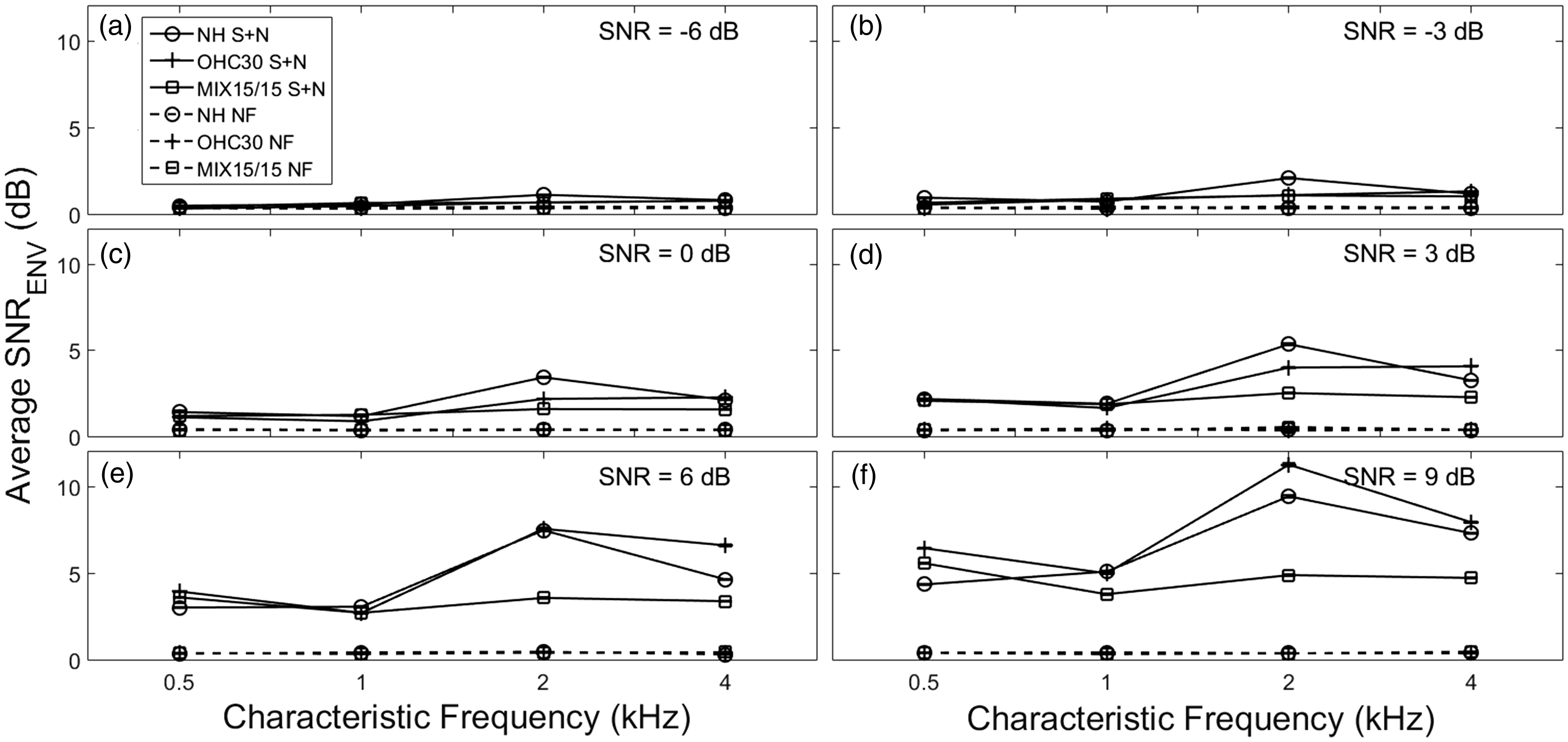
Representation of the acoustic waveforms and corresponding AN-model synapse outputs sampled for a fiber with 2-kHz CF. The sentence presented was “The grass curled around the fence post.” Each column corresponds to a different acoustic input signal-to-noise ratio (SNR): (a) −3 dB, (b) 0 dB, (c) 9 dB. For each column, the topmost panel shows the three signal waveforms (from top to bottom): Clean speech (S), noisy speech (S + N), and noise alone (N). In these panels, the ordinate represents stimulus amplitude in pascals (Pa). Each signal within the subplot is offset by 0.1 Pa for visual purposes. The three bottom panels in each column show the corresponding AN-model (normal hearing) synapse output for each signal.

Figure 2.

Neural modulation coding of non-periodic stimuli can be quantified from spike-train responses of single auditory-nerve fibers using shuffled correlogram analyses. The shuffled-correlogram sumcor (top) was used to quantify temporal envelope coding in each response. The envelope power spectral density (PSD) is computed as the Fourier transform of the sumcor (bottom) and provides a representation of the modulation spectrum of the neural response.

Figure 3.

Neural spike-train analyses showed patterns of modulation coding for noisy speech that were similar to the envelope power spectrum model for speech (sEPSM, Jørgensen & Dau, 2011). Envelope power (in dB) as a function of modulation band center frequency (MF, in Hz), averaged across all 100 sentence presentations (10 sentences ×10 iterations) is shown for a medium-SR model AN fiber averaged across characteristic frequencies. Each subplot represents a different acoustic input signal-to-noise ratio (SNR): (a) −3 dB and (b) 3 dB, for clean speech (S, solid black lines with filled symbols), noisy speech (S + N, dashed lines with unfilled symbols), and N (dotted lines with filled symbols) from each hearing condition: (i) normal hearing (NH, squares), (ii) outer hair cell dysfunction alone (OHC30, triangles), and (iii) mixed outer and inner hair cell dysfunction (MIX15/15, circles).

Figure 4.

Individual differences in speech intelligibility are predicted with varying degrees of OHC/IHC dysfunction. Total neural envelope signal-to-noise ratio (SNR_ENV) in dB is plotted as a function of acoustic input SNR (in dB), averaged across 100 sentence presentations (10 sentences ×10 iterations). The solid lines represent the predicted SNR_ENV of noisy speech (S + N), and the dashed lines represent the predicted SNR of the neural noise floor computed from randomized spike times (NF). Three versions of the AN model that varied in OHC/IHC dysfunction are represented by a different line: normal hearing (NH, no symbol), outer hair cell dysfunction alone (OHC30, circles), and mixed outer and inner hair cell dysfunction (MIX15/15, cross marks). All comparisons were made at equal SL, using medium-spontaneous-rate fibers. The error bars represent the standard error of the mean SNR_ENV.

Figure 5.

Envelope signal-to-noise ratio (SNR_ENV) varies non-monotonically with modulation frequency (MF). Average SNR_ENV (in dB) is plotted as a function of MF (in Hz), averaged across 100 sentence presentations (10 sentences ×10 iterations) and the four model AN-fiber center frequencies (CFs). The SNR_ENV for the noisy speech (S + N) signal is represented by solid lines, and the SNR_ENV for the neural noise floor (NF) is represented by dashed lines. Each hearing condition is represented by a different line and symbol: normal hearing (NH, circle), outer hair cell dysfunction alone (OHC30, plus sign), and mixed outer and inner hair cell dysfunction (MIX15/15, square). Each panel from (a–f) corresponds to a different acoustic input SNR.

Figure 6.

Envelope signal-to-noise ratio (SNR_ENV) varies non-monotonically with model AN-fiber center frequency (CF). Average SNR_ENV (in dB) is plotted as a function of CF (in kHz), averaged across 100 sentence presentations (10 sentences ×10 iterations) and the seven modulation frequencies (MFs). The SNR_ENV for the noisy speech (S + N) signal is represented by solid lines, and the SNR_ENV for the neural noise floor (NF) is represented by dashed lines. Each hearing condition is represented by a different line and symbol: normal hearing (NH, circle), outer hair cell dysfunction alone (OHC30, plus sign), and mixed outer and inner hair cell dysfunction (MIX15/15, square). Each panel from (a-f) corresponds to a different acoustic input SNR.

Figure 7.

Spike-train analyses of the sEPSM model allow for the effects of individual differences in cochlear hearing losses to be explored as a function of AN-fiber characteristic frequency (CF) and neural modulation frequency (MF). SNR_ENV (in dB), averaged across 100 sentence presentations (10 sentences ×10 repetitions) is shown for each CF (in kHz) and MF (in Hz). Each row represents a different hearing condition: normal hearing (NH), outer hair cell dysfunction alone (OHC30), mixed outer and inner hair cell dysfunction (MIX15/15). Each column corresponds to a different acoustic input SNR: (panels a–c) 0 dB, (panels d–f) 6 dB, (panels g–i) 9 dB. The grayscale bar on the right represents the average SNR_ENV range (in dB) across all conditions—lighter regions correspond to a lower SNR_ENV, whereas darker regions correspond to a higher SNR_ENV.

One of the most challenging perceptual consequences of SNHL is the reduced ability to understand speech in background noise due to diminished temporal coding of AN fibers with hearing impairment (Henry & Heinz, 2012). The ability to discriminate speech in noise generally worsens as the degree of hearing loss increases (Dubno, Dirks, & Morgan, 1984; Hornsby, Johnson, & Picou, 2011). However, two individuals who have the same configuration and degree of hearing loss as shown on an audiogram can vary dramatically in their ability to discriminate speech in noise (Dubno & Dirks, 1989). These individual differences may result (at least partially) from differences in the underlying cochlear pathology (e.g., pure OHC dysfunction vs. mixed OHC/IHC dysfunction, resulting in the same loss of sensitivity but with different spectral and temporal coding). The loss of audibility from cochlear hearing loss is thought to be independent from the loss of signal-to-noise ratio (SNR loss) that also occurs as a suprathreshold consequence of cochlear damage, resulting in the distortion of speech (Killion & Niquette, 2000). Although a current notion often applied to interpreting clinical SNR loss is that hearing loss up to ∼60 dB HL is only OHC based and any degree of HL greater than 60 dB is caused by damage to IHCs, this idea regarding SNR loss has not been tested with a physiologically based model that includes the known physiological effects of OHC and IHC dysfunction.

Speech can be characterized in terms of its envelope (slowly varying fluctuations in amplitude over time) and fine structure (rapidly changing fluctuations). Envelope cues are thought to be encoded as fluctuations in the short-term firing rate of AN fibers and to convey information regarding basic speech characteristics such as phonemes, syllables, and words. When speech and noise are present together in the signal, these slowly varying fluctuations in speech are affected by the noise (Dubbelboer & Houtgast, 2007; Houtgast & Steeneken, 1973). Dubbelboer and Houtgast (2007) showed that in addition to reducing the fluctuations in speech, the noise waveform creates new stochastic modulations and interactions with the speech waveform, both of which are thought to affect speech intelligibility. Therefore, techniques such as the speech transmission index (STI; Steeneken & Houtgast, 1980) that account only for the reductions in speech modulations, or measures such as the articulation index (AI; French & Steinberg, 1947) and speech intelligibility index (American National Standards Institute [ANSI], 2007) that measure speech and noise levels individually and do not factor in modulations, are not always able to predict speech recognition in noise accurately (reviewed by Assmann & Summerfield, 2004).

Recent psychophysically based modeling demonstrated that the SNR at the output of a modulation filter bank (SNR_ENV) provides a robust measure of speech intelligibility (Jørgensen & Dau, 2011; Jørgensen, Ewert, & Dau, 2013). The speech-based envelope power spectrum model (sEPSM) assumes that the effect of the noise (N) on speech (S) coding is to (a) reduce envelope power of S + N by filling in the dips of clean speech and (b) introduce a noise floor due to intrinsic fluctuations in the noise itself. Changes in the SNR_ENV metric with acoustic processing or distortion were related to a change in speech reception threshold. An ideal-observer framework was used to convert SNR_ENV to percent correct. The central hypothesis of this modeling framework was that the predicted change in intelligibility arises because the processing changes the input (acoustic) SNR needed to obtain the SNR_ENV corresponding to a given percent correct. SNR_ENV predicted speech intelligibility across a wider range of degraded conditions than many long-standing speech-intelligibility models (e.g., STI). Key insight into the effect of spectral subtraction on speech intelligibility was garnered by consideration of the modulation-domain SNR, which factors in the inherent fluctuations within the noise. Although spectral subtraction increased the envelope power in the noisy-speech (leading STI-based metrics to predict improvements), it also increased the envelope power in the noise-alone response to a greater degree such that SNR_ENV decreased, consistent with the observed performance degradation.

While the sEPSM has been successful in using the SNR_ENV metric to predict speech intelligibility in noise for normal-hearing listeners (Jørgensen & Dau, 2011; Jørgensen et al., 2013), this modeling approach has not yet been extended completely to study the effects of SNHL. One reason the sEPSM has not been extended to SNHL is because of the limited understanding of how different types of SNHL affect envelope coding of speech in noise (S + N) and of noise alone (N). To evaluate the effects of various types of SNHL on envelope coding of speech in noise, it is necessary to (a) consider responses at the level of the AN to include the important aspects of SNHL related to both OHC and IHC dysfunction and (b) quantify envelope coding in responses to non-periodic stimuli. Computational models of AN-fiber responses now exist that incorporate the salient response properties (both rate and timing) that are important for modeling individual differences based on much of what is known about OHC/IHC dysfunction (reviewed by Heinz, 2010, 2016). Additionally, shuffled correlograms provide robust temporal analyses of spike-train responses to non-periodic stimuli (Heinz & Swaminathan, 2009; Joris, 2003; Louage, van der Heijden, & Joris, 2004), which have been applied to quantifying both temporal fine structure and temporal envelope coding of speech-in-noise stimuli (Swaminathan & Heinz, 2011, 2012). In fact, these analyses were used to predict differences in the effects of OHC and IHC dysfunction in across-channel envelope coding within different modulation bands (Swaminathan & Heinz, 2011). Although those predictions were interpreted to have implications for speech-in-noise coding, they lacked a quantitative theoretical framework for relating them to speech intelligibility.

The current study extended the acoustic sEPSM model analysis of SNR_ENV to model neural spike-train responses in normal-hearing and hearing loss conditions. The goals of this study were twofold: (a) to establish the feasibility of computing a neural SNR_ENV metric from single AN-fiber spike-train responses and (b) to make predictions as to whether individual differences in speech intelligibility are likely to occur between similar audiometric hearing losses (degree and configuration) that differed in the relative contributions of OHC and IHC dysfunction.

Methods

Stimuli

Ten sentences from the Harvard test sentence database were used in this study (IEEE Audio and Electroacoustics Group, 1969). The sentences were spoken by a female talker and recorded in a single channel at a 44.1-kHz sampling rate, using a Lynx TWO™ soundcard. The stimuli were down-sampled to 22.05 kHz before being combined with noise. Speech-shaped noise (SSN) was generated in three steps—first, the 10 sentences were concatenated and linear predictive coding (LPC) analysis was used to extract 126 LPC coefficients that describe the long-term average speech spectrum for these 10 sentences. Second, a Gaussian white noise was created with the same duration as the concatenated sentences. Third, the white noise was filtered using the LPC coefficients for the long-term average speech spectrum to obtain SSN. As required for the sEPSM model (Jørgensen & Dau, 2011), speech-in-noise (S + N) and noise-alone (N) stimuli were generated from each clean sentence (S) to create three stimulus conditions for each sentence (Figure 1, top panels). Speech-in-noise sentences were generated by adding a random section of the SSN to each sentence in quiet. Clean speech sentences were calibrated for the AN model to be either 50 dB SPL or 80 dB SPL, depending on hearing condition, as described later. Varying acoustic input SNR conditions were created by adjusting the noise level for each acoustic SNR.

AN Model

The Zilany, Bruce, and Carney (2014) AN model was used in this study because it is a well-established phenomenological model representing the signal processing in the peripheral auditory system from the middle ear to the AN. This AN model incorporates several non-linear processes related to the cochlear and AN processing, such as compression, suppression, level-dependent tuning, neural adaptation, and so forth, and has been shown to provide an excellent representation of neural envelope coding based on its synaptic power-law dynamics (Zilany, Bruce, Nelson, & Carney, 2009; Zilany & Carney, 2010). The model also allows the simulation of different types of SNHL with varying degrees of OHC and IHC damage. The AN model takes a sound signal (in Pa) as input and generates spike times at the level of the IHC-AN synapse, for a given fiber characteristic frequency (CF) and spontaneous rate (SR) type.

For the purposes of this preliminary study, spike times from AN fibers were generated from model fibers with four CFs (0.5 kHz, 1 kHz, 2 kHz, and 4 kHz). This limited set of CFs was chosen for simplicity to demonstrate these new neural analyses, while being representative of the audiometric range of frequencies pertaining to speech. Since one of our goals is to understand the effects of SNHL, three hearing conditions were tested: (a) normal hearing (NH), (b) a flat 30-dB hearing loss due to OHC damage alone (OHC30), and (c) a flat 30-dB hearing loss due to an equal degree (15-dB each) of OHC and IHC damage (MIX15/15). In the AN model, hearing loss was incorporated at all CFs by specifying the parameters for OHC and IHC dysfunction (C_OHC and C_IHC, respectively). Table 1 specifies the exact values used for each CF in each condition corresponding to the hearing threshold. Clean speech stimuli were calibrated to represent equal sensation levels (SLs) for all conditions: 50 dB SPL for the normal-hearing condition and 80 dB SPL for both of the hearing loss conditions. Unlike a typical clinical prescription, a flat gain was applied across all frequencies in order to control for audibility directly by equating SL. Based on correlogram analyses of the responses of the specific AN fibers used in this study (described later), these SPL values correspond very closely to the best modulation level (BML) for these model AN fibers for all conditions considered here.

Table 1.

Parameters Used to Represent Varying Degrees of OHC and IHC Dysfunction in the AN model.

	COHC				CIHC
CF (kHz)	0.5	1	2	4	0.5	1	2	4
NH	1	1	1	1	1	1	1	1
OHC30	0	0.09	0.15	0.15	0.3	1	1	1
MIX15/15	0.10	0.40	0.40	0.45	0.20	0.15	0.20	0.15

Note. Parameters used are C_OHC and C_IHC, where 1 represents normal function and 0 represents complete dysfunction, respectively. Values varied across AN-fiber CF and the three hearing conditions considered in this study. Note that because the AN model includes less than 30 dB of cochlear amplifier gain for the 500-Hz CF (Zilany & Bruce, 2007b), C_IHC was less than 1 for this CF to achieve the 30-dB total hearing loss in this fiber. NH = normal hearing; OHC30 = 30-dB flat hearing loss due to OHC dysfunction alone; MIX15/15 = 30-dB flat hearing loss due to equal degrees of OHC and IHC dysfunction; AN = auditory-nerve; OHC = outer hair cell; IHC = inner hair cell; CF = characteristic frequency.

The AN model provides options for different SR types (high: 100 spikes/s, medium: 5 spikes/s, and low: 0.1 spikes/s; Zilany et al., 2009). In this initial feasibility study, medium-SR model AN fibers were used since they represent a balance between the hard saturation of high-SR fibers and the low spike rates of low-SR fibers. All stimuli were resampled to 100 kHz to match the sampling rate of the AN model (Zilany et al., 2014).

Figure 1 (bottom panels) shows the AN-model-fiber synapse output from a medium-SR fiber with a 2-kHz CF, responding to the three stimulus conditions, clean speech (S), noisy speech (S + N), and noise alone (N), based on the sentence “The grass curled around the fence post.” Each column represents a different acoustic input SNR: (a) −3 dB, (b) 0 dB, and (c) 9 dB. The waveforms represent model AN-fiber output from the NH condition. In each subfigure, the topmost panel shows the acoustic waveforms for the three stimulus conditions with clean S (light gray) at the top, followed by S + N (black), and N alone (dark gray). The bottom three panels in each column show the corresponding AN-model synapse outputs for the three stimulus conditions. Certain differences are visible when a comparison is made across different acoustic input SNRs. The increase in input SNR going from Figure 1 (a) to (c) is seen in the reduction in noise in the S + N and N waveforms, with the speech remaining constant throughout. The corresponding AN-model synapse output for S + N is seen to resemble that of S, especially at the 9 dB SNR. In terms of envelope coding, it can be seen that the AN-fiber output follows the acoustic envelope of the corresponding signal waveform. Although the N itself is relatively steady state, there are some intrinsic short-term fluctuations captured in the AN synapse output. Comparing the spike output of S with that of S + N, it can be seen that the larger modulations in the clean S are also present in S + N (e.g., between the vertical dashed lines at ∼0.2 and 0.4 seconds). On the other hand, smaller modulations are typically embedded in the noise (e.g., between ∼1.75 and 1.8 seconds). Based on the sEPSM model (Jørgensen & Dau, 2011), the relative envelope coding between speech and the inherent noise fluctuations, as captured by the SNR_ENV metric, is an important predictor of speech understanding. The main purpose of this initial study is to develop quantitative neural spike-train analyses to compute the SNR_ENV metric from neural spike trains so that the effects of different types of SNHL (e.g., OHC vs. IHC dysfunction) can be quantified in the sEPSM framework.

Predicting SNR_ENV From Model Auditory-Nerve-Fiber Spike-Train Responses

To replicate the general procedure for obtaining the SNR_ENV metric in the sEPSM model (Jørgensen & Dau, 2011), it is necessary to quantify envelope coding from single AN-fiber spike-train responses to non-periodic stimuli, such as S + N. Shuffled correlogram analyses (e.g., Joris, 2003; Louage et al., 2004; Swaminathan & Heinz, 2011) were used to quantify envelope coding in each of the three stimulus conditions (S, S + N, and N) for each sentence. Model spike trains were obtained for each stimulus in response to the original stimulus (positive) and its polarity-inverted pair (negative). For each stimulus, a total of 1,500 spike times were collected across 100 stimulus repetitions. Shuffled auto correlograms and shuffled cross-polarity correlograms (SCCs) were used to quantify temporal coding for each set of spike trains for a given CF. To isolate envelope coding, a sumcor was computed by averaging the shuffled auto correlograms and shuffled cross-polarity correlograms (i.e., emphasizing the similarities in temporal envelope coding between the positive and negative polarity responses; Joris, 2003; Louage et al., 2004). The sumcor thus quantifies temporal envelope coding in terms of an autocorrelation function (Figure 2 top). The modulation spectrum of the neural response can be estimated by computing the Fourier transform of the sumcor, since the Fourier transform of an autocorrelation function is the power spectral density (PSD) of the signal (Rangayyan, 2001). Here, the envelope PSD was computed based on sumcors computed out to ±1-second delays to achieve 1-Hz spectral resolution (Figure 2, bottom). For a more detailed description of these neural methods for envelope and modulation-spectrum analyses, see Swaminathan and Heinz (2011).

As in the sEPSM analyses (Jørgensen & Dau, 2011), the total SNR_ENV metric for each stimulus condition was computed by combining individual SNR_ENV values for each cochlear CF and modulation-filter center frequency (MF). In the neural domain, the AN-fiber CF defined cochlear CF, and the neural PSD provides the modulation spectrum from which modulation power within individual modulation bands (filters) can be computed. Here, envelope power was computed within seven modulation-frequency bands (MF) by integrating the envelope PSD within different MF ranges (a low-pass range at and below 1 Hz, and six octave-spaced bands centered at MFs of 2 to 64 Hz with a bandwidth equal to the center frequency, i.e., Q = 1). Although not implemented directly as modulation filters, these seven modulation bands correspond closely to the seven original modulation bands from the sEPSM approach (Jørgensen & Dau, 2011). For each CF and MF, the envelope SNR, SNR_ENV(CF, MF) was computed by subtracting the envelope power of N from the envelope power of S + N and dividing the result by the envelope power of N (see Equations (2) and (4) in Jørgensen & Dau, 2011). To verify significant envelope coding in each CF and MF band, for each sentence, a neural noise floor was computed to provide a baseline for comparison against the power obtained from the stimulus. For each set of stimulus-driven spike trains, a set of randomized spike trains was generated that included uniformly distributed spike times within each repetition, where the number of spikes in each repetition was maintained (i.e., keeping the same amount of data, but removing any temporal structure within the spike trains). The neural noise floor for each CF and MF was computed from PSDs derived from sumcors of the randomized spike trains. If the total S + N power within a modulation band was within 10% of the neural noise floor power within that MF band, the band was not allowed to contribute to the total SNR_ENV value. Here, the model analyses consisted of seven MFs (Figure 3) and four CFs (i.e., 28 individual SNR_ENV values). To obtain a final value (total SNR_ENV), the individual SNR_ENV(CF, MF) values were combined by taking the square root of the sum of the squares of the significant individual SNR_ENV(CF, MF) values (as in Equation (6) of Jørgensen & Dau, 2011). The total SNR_ENV was also calculated from the random spike times using the same steps to create a neural SNR_ENV noise floor (Figure 4).

Statistical Analysis

Data were collected for 10 iterations of the AN model responding to each of the 10 sentences, yielding data from 100 presentations. Initial multiple linear regression (MLR) modeling determined that there was no effect of iteration, representing only neural variability in the 10 different sets of spike trains in response to each sentence. Thus, all remaining analyses were based on average SNR_ENV values across the 10 iterations. Seven different acoustic input SNR conditions were tested: −9, −6, −3, 0, 3, 6, and 9 dB SNR to evaluate the effect of input SNR on SNR_ENV. Statistical analyses were carried out using JMP (SAS) to evaluate fits of MLR models that predicted SNR_ENV from the categorical variable of hearing condition and the continuous variable of acoustic input SNR. The model incorporated the interaction term between hearing condition and input SNR, as well as the random effects of sentence using restricted maximum likelihood fits. Sentence was included as a random-effects variable because the effect of sentence, while significant, was not part of our primary hypothesis testing. Residuals of these regression models were normally distributed with comparable variance. Adjusted R² was used to quantify the degree of association between the explanatory variables and the total SNR_ENV.

Results

Neural Analyses Showed Similar Speech-In-Noise Modulation-Coding Patterns to the sEPSM Model

Figure 3 shows the average envelope power across all sentences for S, S + N, and N conditions at input SNRs of −3 dB (left) and 3 dB (right) for the average of four CFs. Within each stimulus condition, the three lines represent the three hearing conditions. The envelope power for S was the greatest followed by the envelope power for S + N and then for N. In general, a peak in the clean speech envelope power was observed in the 4-Hz modulation band. These results are consistent with the modulation excitation patterns for S, S + N, and N in the sESPM model (Jørgensen & Dau, 2011). Among the hearing conditions, the NH condition had the greatest power followed by OHC30 and MIX15/15. Also, of critical importance for the sEPSM model is the difference between the power of the S + N and N conditions. At the lower MFs (1-8 Hz), the power for S + N was higher than the power for N. This difference between S + N and N for a given CF and MF creates a positive SNR_ENV (CF, MF). However, for MF ≥ 16 Hz, the envelope power of S + N and N generally overlap, and thus the power at these MFs does not contribute to increasing the overall SNR_ENV.

SNR_ENV Increased Monotonically With Increasing Acoustic Input SNR

Results showed that the total SNR_ENV predicted from the AN-model spike trains increased monotonically as acoustic input SNR was increased from −9 dB to 9 dB, with all predictions being above the flat neural noise floor computed from randomized spike times (Figure 4). This was observed for NH and both the HL conditions; differences across hearing condition are discussed in the next section. There was a highly significant positive correlation between acoustic input SNR and total SNR_ENV for all conditions. Based on the MLR model that included NH and both HL conditions, total SNR_ENV could be predicted from acoustic input SNR (β = 0.635, p < .001). For the NH condition, SNR_ENV values ranged from about 0.8 dB at the lowest acoustic input SNR of −9 dB to 11.4 dB at the highest input SNR of 9 dB. This overall range of SNR_ENV across this input SNR range is similar to the predictions from the sEPSM model for steady-state noise maskers (Jørgensen & Dau, 2011). The SNR_ENV for the OHC30 and MIX15/15 conditions ranged from −0.4 dB to 12.1 dB and 0.2 dB to 9.9 dB, respectively, over the same range of input SNRs.

The Overall Effect of Hearing Loss Was to Decrease SNR_ENV

Both the OHC30 and MIX15/15 conditions generally produced SNR_ENV values below those of the NH model (Figure 4). To test the overall effect of a 30-dB hearing loss on SNR_ENV, a version of the linear regression model predicting SNR_ENV from input SNR and hearing condition was considered where hearing condition was either NH or HL (i.e., HL condition combined the OHC30 and MIX15/15 conditions into a single SNHL category, consistent with audiological classification). This model (Adjusted R²= 0.94, p < .0001) demonstrated negative effects of hearing loss, F(1, 197) = 32.51, p < .0001, and positive effects of acoustic input SNR, F(1, 197) = 2650.00, p < .0001, on SNR_ENV. However, analyses suggest that when these two types of HL were combined into a single category, the effect of HL did not depend on input SNR (hearing condition by input SNR, F(1, 197) = 1.7139, p = .1920.

The Effect of Acoustic Input SNR on SNR_ENV Depended on the Type of Hearing Loss

Predictions of total SNR_ENV as a function of acoustic input SNR (Figure 4) varied across the three AN-model versions with different degrees of OHC/IHC dysfunction. To explore potential effects of individual differences in HL on SNR_ENV, a more specific version of the linear regression model was considered where all three hearing conditions were included in the categorical HL variable. This model (Adjusted R²= 0.96, p < .0001) demonstrated significant main effects of hearing condition, F(2, 195) = 38.08, p < .0001, and acoustic input SNR, F(1, 195) = 4270.56, p < .0001, on SNR_ENV, as well as a significant interaction between hearing condition and input SNR, F(2, 195) = 27.26, p < .0001. At very low input SNRs ( ≤ −6 dB), MIX15/15 SNR_ENV values were below NH, but above OHC30 values. In contrast, above −3 dB input SNR, OHC30 SNR_ENV, values were above the MIX15/15 values. Thus, a crossover was observed between the two HL conditions. This crossover is due to a greater acoustic input SNR loss (rightward shift) in the SNR_ENV versus input SNR function for OHC30 dysfunction at low input SNRs (e.g., more noise through broader filters) and less acoustic SNR loss for cleaner speech (i.e., at higher input SNRs). In contrast to the level-dependent acoustic SNR losses predicted for the OHC30 condition, the MIX15/15 predictions demonstrated a level-independent acoustic SNR loss as the MIX15/15 curve was generally parallel to the NH curve, with a consistent rightward shift of ∼2 dB for this mild hearing loss. To explicitly evaluate whether the SNR_ENV effects of these different types of 30-dB HL depend differently on acoustic input SNR, a version of the linear regression model was evaluated that only included the OHC30 and MIX15/15 conditions in the categorical variable of hearing condition. This model (Adjusted R²= 0.97, p < .0001) demonstrated significant main effects of hearing condition, F(1, 127) = 47.50, p < .0001, and acoustic input SNR, F(1, 127) = 4603.94, p < .0001, on SNR_ENV, as well as a significant interaction between hearing condition and input SNR, F(1, 127) = 81.49, p < .0001). Thus, these analyses suggest that different types of 30-dB audiometric hearing losses (i.e., arising from differing degrees of OHC/IHC dysfunction) can have acoustic SNR losses that depend on input SNR in different ways.

SNR_ENV Varied Non-Monotonically With MF

These spike-train analyses of the sEPSM model allow for the exploration of individual differences in the MF domain for noisy-speech encoding. To do so, individual SNR_ENV values were collapsed across CFs for each iteration of each sentence. This was done by calculating the square-root of the sum of squares of the SNR_ENV values of all CFs for a given MF. This value was further averaged across sentences and iterations to provide an average SNR_ENV as a function of MF (Figure 5). In general, at each acoustic input SNR, the relationship between SNR_ENV and MF was non-monotonic. Figure 5 shows this relationship at input SNRs from −6 dB to 9 dB (panels a–f). In all panels, SNR_ENV increased with increasing MF up to 4 Hz, reaching peak values between 0.5 dB for NH (at −6 dB SNR) to 10.4 dB for OHC30 (at 9 dB SNR). In general, SNR_ENV decreased as MF increased beyond 4 Hz. For input SNRs between −6 dB and 3 dB, the SNR_ENV for NH was greater than the HL conditions for MFs between 2 and 8 Hz. At 6 dB input SNR, the SNR_ENV for the OHC30 condition was higher than the other two conditions for MF = 4 Hz, whereas for 9 dB input SNR, this was true for both 2 and 4 Hz MF. In general, there were only very small differences across HL condition for MFs of 1 Hz and MFs of 16 Hz and above.

SNR_ENV Varied Non-Monotonically With Model AN-fiber CF

To examine the dependence of SNR_ENV on CF, individual SNR_ENV values were collapsed across the seven MFs for each iteration of each sentence. For a given CF, the square-root of the sum of squares of the SNR_ENV at each MF was obtained. This value was averaged across iterations and sentences to obtain an average SNR_ENV as a function of CF. Figure 6 shows that the SNR_ENV was generally highest for the 2-kHz CF for all acoustic input SNRs. Overall, the increase in SNR_ENV with increasing acoustic input SNR appears to be driven predominantly by the 2-kHz CF for input SNRs ≤ 0 dB, with peak values ranging from 0.7 dB for NH (−9 dB SNR) to 11.3 dB for OHC30 (9 dB SNR). At the highest input SNRs of 6 dB and 9 dB, the SNR_ENV for the OHC30 condition was higher than the NH condition. The differences in SNR_ENV between HL conditions were greatest at 2 kHz followed by 4 kHz.

More detailed analyses of the dependence of the SNR_ENV effects of HL condition across CF and MF can be explored with these spike-train analyses of the sEPSM model. Figure 7 shows a matrix of SNR_ENV values as a function of MF and CF for each hearing condition (rows), at three different acoustic input SNRs (columns: 0 dB, 6 dB, 9 dB). The SNR_ENV matrices in Figure 7 generally show darker regions corresponding to the 2-kHz CF relative to lighter regions at the other CFs. Looking across MF, as discussed earlier, it can be seen that the best SNR_ENV values were generally achieved between MFs of 2 to 8 Hz. In general for these preliminary predictions, the patterns of variation in SNR_ENV across CF and MF were similar across the HL conditions; however, detailed analyses of this type are required to fully explore the source of individual differences predicted with the neural sEPSM model.

Discussion

Speech-Based Envelope Power-Spectrum Model Predictions From Neural Spike Trains Are Generally Consistent With the Psychophysically Based Predictions

The SNR_ENV metric from the sEPSM has been shown to have great promise for predicting speech intelligibility for normal-hearing listeners (Jørgensen & Dau, 2011); however, it has not yet been thoroughly extended to hearing-impaired listeners due to limitations in our physiological knowledge of how SNHL affects the envelope coding of speech in noise (specifically in relation to N). In the present study, envelope coding to non-periodic stimuli (e.g., speech in noise) was quantified from AN-model spike trains using shuffled-correlogram analyses. The envelope-based correlograms (i.e., estimated envelope autocorrelation functions) were analyzed in the MF domain to compute modulation-band based estimates of signal and noise envelope coding (e.g., a neural SNR_ENV metric computed in the same manner as the SNR_ENV metric from the sEPSM).

Overall, many aspects of the SNR_ENV predictions computed here from neural spike trains showed close similarities to the psychoacoustical model predictions motivating this work (Jørgensen & Dau, 2011). First, envelope-power excitation patterns (Figure 3) showed the same relative position across stimulus conditions, with the highest envelope power for S, the lowest envelope power for N, and S + N in between. These findings support the assumptions that the effect of the noise on speech coding is to (a) reduce envelope power by filling in the dips of S and (b) introduce a noise floor due to intrinsic fluctuations in the noise itself (Figure 1). As the acoustic input SNR decreased, the neural firing to the S + N condition became less similar to the S response, and thus although the envelope power for S did not change (because the presentation level for S was fixed), the envelope power for S + N approached that for N (Figure 3). This observation is in accordance with the theory that noise reduces the overall envelope power of the S + N signal compared with S (Jørgensen & Dau, 2011). Second, the peak in speech envelope power (Figure 3) was generally observed in the 4-Hz modulation band (consistent with the syllabic modulation rate in speech). The resultant SNR_ENV also generally peaked at 4 Hz (Figure 5) but was significant between 2 and 8 Hz MF, consistent with the psychoacoustical predictions (Jørgensen & Dau, 2011). With this acoustic model, time-averaged SNR_ENV was high for the 1 to 8 Hz MFs for a SSN masker (Jørgensen et al., 2013). The discrepancy in SNR_ENV at 1 Hz may result from the maximum delay of 1 second used in the neural correlograms, which may limit the spectral resolution around 1 Hz and appears to produce an unexpectedly high envelope power at 1 Hz MF relative to 2 Hz (Figure 3) in comparison to the sEPSM predictions. Third, as seen in Figure 7 of Jørgensen and Dau (2011), negligible differences were predicted between noisy-speech and noise-alone envelope power (i.e., zero SNR_ENV in Figure 5) for the 16 to 64 Hz modulation bands (Figure 3). Fourth, the total neural SNR_ENV varied from about 1 dB to 14 dB as acoustic (input) SNR varied from −9 to 9 dB, with these neural values being above the neural noise floor in all conditions (Figure 4). Thus, the neural SNR_ENV metric replicates the main properties seen in the psychoacoustical predictions and thus provides a means to account for the relative strength of the intrinsic neural fluctuations due to the noise in relation to the coding of speech modulations.

Individual SNHL Differences in SNR_ENV Varied Across Acoustic Input SNR

Three hearing conditions with varying degrees of OHC/IHC dysfunction were evaluated in this study: normal hearing (NH), and two mild SNHL conditions, pure 30-dB OHC dysfunction (OHC30) and mixed 30-dB OHC-IHC dysfunction (MIX15/15). Preliminary results predict that even these mild SNHL conditions affect speech intelligibility in noise at equal-SL conditions, as characterized by the sEPSM metric SNR_ENV (Figure 4). More importantly, the present predictions provide insight into the possibility of individual differences in speech intelligibility for similar degrees of hearing loss arising from differing degrees of OHC and IHC dysfunction. All three hearing conditions showed increases in SNR_ENV with increasing acoustic input SNRs, and in fact when both the OHC30 and MIX15/15 hearing loss conditions were combined into a single SNHL category (as is typical in audiological assessment), there was no interaction between the effects of hearing condition and input SNR. This result suggests that the effect of SNHL on SNR_ENV does not depend on input SNR and would support the use of a single SNR-loss value to characterize the suprathreshold effects of SNHL on speech intelligibility.

In contrast, when the two types of SNHL were considered as separate categories of hearing condition, in isolation or in addition to normal hearing, there was a significant interaction between hearing condition and input SNR, suggesting that the effect of hearing condition on SNR_ENV varies across input SNR. In this more physiologically specific case, a single value of SNR loss (e.g., evaluated at SNR_ENV = 5 dB, dotted line in Figure 4) is not sufficient to characterize the effects of SNHL. These results suggest that the inclusion of IHC dysfunction in this AN model (i.e., shallower IHC transduction; Bruce, Sachs, & Young, 2003) can have a significant effect on speech-intelligibility predictions. This type of shallower IHC transduction is likely to occur (in addition to OHC dysfunction) in a wide range of SNHL etiologies, such as noise-induced, metabolic presbycusis, and ototoxic hearing loss and thus is important to include in modeling studies of SNHL (Heinz, 2010, 2016). The steeper rate of growth in SNR_ENV with input SNR for the OHC30 condition is the primary cause of the input-SNR-dependent effects and is likely due to broader cochlear filters that are more susceptible to noise at low SNRs and become less relevant for higher SNRs (i.e., for S). Although the details of these preliminary predictions should not be over-interpreted, the consistent finding of differences in the rate of SNR_ENV growth with input SNR suggests that it may be necessary to characterize speech intelligibility across a range of input SNRs in order to diagnose fully the individual differences in types of SNHLs (e.g., with varying degrees of OHC/IHC dysfunction).

Summary, Limitations, and Future Directions

The present study extended the successful sEPSM analyses to the neural domain so that the important effects of inherent noise fluctuations on speech intelligibility can be predicted from spike-train data. Modeling at the AN level or above is required to include the peripheral physiological factors known to influence neural coding of complex sounds: (a) OHC dysfunction, (b) IHC dysfunction, (c) IHC loss (dead regions), (d) endocochlear potential reduction in presbycusis, and (e) cochlear synaptopathy. This study predicted that the inclusion of the shallower transduction function associated with many forms of mild-moderate IHC dysfunction (i.e., less severe than IHC dead regions) can affect speech-intelligibility predictions in addition to the inclusion of OHC dysfunction. Furthermore, the spiking output produced at the synapse of the Zilany et al. (2014) AN-model incorporates processes such as neural adaptation and spontaneous-rate variations that affect modulation coding, in addition to cochlear suppression, which are generally unaccounted for by psychoacoustic analyses of speech intelligibility. While the preliminary neural predictions shown here were primarily to demonstrate the feasibility of neural SNR_ENV computations from spike-train responses, the crossover in Figure 4 suggests that individual differences may occur based on differential degrees of OHC/IHC dysfunction in listeners currently diagnosed into the single category of SNHL.

Although the present predictions provide general insight into individual differences, several limitations exist in this approach, which need to be addressed in future studies. A fundamental limitation of autocorrelation based approaches is that they are limited to long-term coding effects and are thus limited to predicting overall performance rather than examining specific confusion patterns based on individual speech features. This is the same limitation faced by well-established frameworks, for example, the articulation index and STI, for predicting the effects of degradations in speech communication channels on overall speech intelligibility (reviewed by Assmann & Summerfield, 2004). Other modeling approaches do exist that compare normal and impaired AN population responses in a spectro-temporally specific manner. For example, the spectro-temporal modulation index (Elhilali, Chi, & Shamma, 2003) was developed to predict speech intelligibility based on cortical representations of spectro-temporal modulations in speech. The spectro-temporal modulation index approach has been extended to predict the effect of presentation level and cochlear impairment on speech intelligibility by using a more physiologically realistic AN model (Zilany & Bruce, 2007a). Also, the neural similarity index measure (Hines & Harte, 2012) has been used to predict speech intelligibility based on slow and fast time-scaled neurograms, which allows individual speech features to be examined (e.g., onset cues, which have been shown to be important in neural responses to certain phonemes; Delgutte & Kiang, 1984), However, these approaches have not been tested across as wide a range of conditions as the sEPSM in terms of their ability to account for the perceptually relevant effects of inherent noise fluctuations on speech intelligibility (Jørgensen & Dau, 2011; Jørgensen et al., 2013).

Another limitation in the present study is the inclusion of only four CFs and only medium-SR AN fibers. This restriction was applied in order to provide a simple demonstration of the feasibility of computing SNR_ENV values from neural spike trains that captured the main features seen in the original psychophysically based sEPSM study (Jørgensen & Dau, 2011). The 50-dB and 80-dB SPL sound levels chosen for this study provided sound levels near the BML for the medium-SR fiber chosen and avoided the common confounds of single-unit AN-fiber threshold or saturation effects that occur due to the limited dynamic range of individual AN fibers. Presenting stimuli at BML is a common modeling approach (Swaminathan & Heinz, 2012) that quantifies the effects of various factors (e.g., input SNR and hearing loss) on the maximal envelope coding, for which it is assumed typically occurs in some AN fibers within the total population based on the typical broad range of AN-fiber thresholds (Liberman, 1978). While these simplifications are not expected to affect the general conclusions of the present study, future studies will explore SNR_ENV predictions based on a more complete range of CFs, SRs, and sound levels to generalize these results.

Additional extensions that are needed include extending these neural analyses to fluctuating maskers, based on the success of the multiresolution sEPSM (Jørgensen et al., 2013). This extension is likely to require the inclusion of higher modulation frequencies based on the psychophysically based modeling (Jørgensen et al., 2013), which can easily be included in the correlogram-based analyses of temporal envelope coding (Swaminathan & Heinz, 2011). Also, one limitation of the sEPSM model is the insensitivity to phase manipulations, which have been overcome in the short-time objective intelligibility measure (Taal, Hendriks, Heusdens, & Jensen, 2011). Such correlation-based decision metrics can be explored in the neural domain using the neural crosscorrelation metrics developed for envelope coding (Heinz & Swaminathan, 2009). Beyond these analysis extensions that have been developed in the psychoacoustical domain, the Zilany et al. (2014) AN model provides a great degree of flexibility in incorporating different combinations of cochlear impairment. This enables the SNR_ENV metric to be expanded to analyze a wider range of audiometric threshold shifts and OHC/IHC dysfunction configurations. Beyond additional predictions from the existing model, the feasibility demonstrated here supports the application of these neural analyses in future animal studies to quantify the effects of various types of SNHL (noise-induced, ototoxic, etc.) on the coding of speech and inherent noise modulations, which will provide invaluable insight for understanding individual differences in speech-in-noise intelligibility and for extending existing models. One specific form of SNHL not able to be analyzed in the current single-unit AN-fiber framework is cochlear synaptopathy that can occur following moderate noise exposure or aging (Kujawa & Liberman, 2015). The effects of this form of hidden hearing loss, which have been predicted to affect neural envelope coding (Bharadwaj, Masud, Mehraei, Verhulst, & Shinn-Cunningham, 2015; Bharadwaj, Verhulst, Shaheen, Liberman, & Shinn-Cunningham, 2014), could however be evaluated easily in moderate-noise-exposed animal studies at the level of ventral cochlear nucleus, or through the addition to the current modeling framework of a computational model of ventral cochlear nucleus responses that includes the effects of convergence (e.g., Rothman, Young, & Manis, 1993). Finally, another application for these analyses would be to predict speech intelligibility outcomes for listeners with SNHL using various signal-processing techniques for the purpose of improving hearing-aid fitting and the development of novel amplification strategies for a variety of real-world listening conditions.