Sage Journals: Discover world-class research

Abstract

Rippled-spectrum stimuli are used to evaluate the resolution of the spectro-temporal structure of sounds. Measurements of spectrum-pattern resolution imply the discrimination between the test and reference stimuli. Therefore, estimates of rippled-pattern resolution could depend on both the test stimulus and the reference stimulus type. In this study, the ripple-density resolution was measured using combinations of two test stimuli and two reference stimuli. The test stimuli were rippled-spectrum signals with constant phase or rippled-spectrum signals with ripple-phase reversals. The reference stimuli were rippled-spectrum signals with opposite ripple phase to the test or nonrippled signals. The spectra were centered at 2 kHz and had an equivalent rectangular bandwidth of 1 oct and a level of 70 dB sound pressure level. A three-alternative forced-choice procedure was combined with an adaptive procedure. With rippled reference stimuli, the mean ripple-density resolution limits were 8.9 ripples/oct (phase-reversals test stimulus) or 7.7 ripples/oct (constant-phase test stimulus). With nonrippled reference stimuli, the mean resolution limits were 26.1 ripples/oct (phase-reversals test stimulus) or 22.2 ripples/oct (constant-phase test stimulus). Different contributions of excitation-pattern and temporal-processing mechanisms are assumed for measurements with rippled and nonrippled reference stimuli: The excitation-pattern mechanism is more effective for the discrimination of rippled stimuli that differ in their ripple-phase patterns, whereas the temporal-processing mechanism is more effective for the discrimination of rippled and nonrippled stimuli.

Keywords

rippled spectra discrimination excitation pattern temporal processing

Introduction

Rippled-spectrum stimuli are exploited as a representative version of complex sound signals. In particular, tests of the ability to detect or discriminate spectral ripples of various ripple densities have been used to measure the spectral resolution of the auditory system. The highest ripple density (the number of ripples per kilohertz or per octave) at which the ripples can be detected or at which two different rippled-spectrum patterns can be discriminated from one another has been assumed to be a measure of the spectral resolution. This test has been used as a measure of the spectral resolution for people with normal hearing (e.g., Supin, Popov, Milekhina, & Tarakanov, 1994, 1998), hearing loss (HL; e.g., Henry, Turner, & Behrens, 2005), and for cochlear implants users (e.g., Anderson, Nelson, Kreft, Nelson, & Oxenham, 2011; Anderson, Oxenham, Nelson, & Nelson, 2012; Litvak, Spahr, Saoji, & Fridman, 2007; Won, Drennan, & Rubinstein, 2007; Won et al., 2014).

The rippled-spectrum test stimuli have been used in several experimental paradigms. In studies by Bilsen and Ritsma (1970), Yost and Hill (1978), Yost (1996), Yost, Hill, and Perez-Falcon (1978), and Yost, Patterson, and Sheft (1996), wideband rippled-spectrum stimuli with equally spaced ripples were used for investigations of the sensation of pitch that matches the frequency spacing between ripples (the repetition pitch). The repetition-pitch limits revealed ripple-pattern resolution with equally spaced ripples.

Many other investigations that have exploited rippled-spectrum test stimuli have not involved subjective estimates of the sound properties such as the repetition pitch. In those cases, the experimental paradigms were based on the discrimination tasks. The task of the listener was to make a choice between a rippled-spectrum test stimulus and a reference stimulus. The stimuli were designed in such a way that the discrimination was possible only when the rippled spectrum pattern of the test stimulus was resolvable. However, there were no commonly accepted ideas for the combinations of test and reference stimuli that should be used for the measurements.

One of the experimental paradigms used both a test and a reference stimuli with rippled spectra of one and the same ripple density. The difference between the stimuli was in the ripple phases. In the test stimulus, the ripple phase periodically shifted or inversed, whereas the ripple phase of the reference stimulus was kept constant. Variation of the ripple pattern allowed determination of the ripple-density resolution limit (ripple peaks and troughs interchanged; Supin, Popov, Milekhina, & Tarakanov, 1994, 1997, 1998, 2003), ripple depth thresholds (Supin, Popov, Milekhina, & Tarakanov, 1999), or ripple-phase shift threshold (Nechaev & Supin, 2013).

Another version of this paradigm was the discrimination between rippled-spectrum stimuli with opposite ripple phases (Anderson et al., 2011; Henry et al., 2005; Jeon, Turner, Karsten, Henry, & Gantz, 2015; Milekhina, Nechaev, & Supin, 2018; Won et al., 2007, 2014). In this case, stimuli could not be specified as the test and reference, and a three-alternative paradigm was used: two stimuli were presented with identical ripple phases and one stimulus with the opposite phase. The task of the listener was to report which of the three stimuli differed from the two others (which stimulus was an oddball). In all of the versions, it was assumed that ripple-phase shifts or differences can only be detected when the ripple pattern is resolvable. When the ripple pattern becomes unresolvable, all the stimuli are perceived as nonrippled, and thus, they cannot be discriminated.

An alternative option was to use a rippled test stimulus and a nonrippled ( flat) reference stimulus. In those cases, the test stimulus either had a constant ripple phase or the ripples glided upward or downward along the frequency scale, or positions of the ripple peaks and troughs at the frequency scale interchanged several times a second (Aronoff & Landsberger, 2013; Chi, Gao, Guyton, Ru, & Shamma, 1999; Nechaev, Milekhina, & Supin, 2018; Van Zanten & Senten, 1983). This experimental paradigm was, in particular, used to measure ripple depth thresholds (Anderson et al., 2012; Litvak et al., 2007; Saoji, Litvak, Spahr, & Eddins, 2009). Similar to the previous case, this paradigm assumes that when the ripple pattern of the test stimulus becomes unresolvable, it is perceived as a nonrippled stimulus, and thus, the test and reference stimuli cannot be discriminated from one another. A version of this paradigm was a reference stimulus with a ripple density that was beyond the resolution limit; such stimuli were expected to be perceived as nonrippled (Aronoff & Landsberger, 2013; Narne, Van Dun, Bansal, Prabhu, & Moore, 2016).

The experimental designs described assumed that both rippled and nonrippled reference stimuli should provide equal or similar results. They implied that the test and reference stimuli can be discriminated from one another when the patterns of rippled-spectrum stimuli are resolvable; the stimuli cannot be discriminated from one another when the rippled patterns are not resolvable. However, it was never checked properly (while keeping other conditions equal), whether these paradigms provide equivalent results. Many investigations referred earlier were performed on different categories of listeners: normal, with various degrees of HL, or with various parameters of cochlear implants. For example, in normal-hearing listeners, with the use of phase-varying test stimuli and rippled reference stimuli, the ripple-density resolution was estimated, depending on the frequency, from 8.1 to 10.6 ripples/oct (Supin et al., 1998), from 5.2 to 10.0 ripples/oct (Supin et al., 1999), and from 8.7 to 9.8 ripples/oct (Milekhina et al., 2018); with constant-phase test stimuli, the estimates were from 2.03 to 7.55 ripples/oct within a wide (0.1–5 kHz) frequency band (Henry et al., 2005) or from 6.2 to 7.8 ripples/oct within a 3-oct band (Milekhina et al., 2018). The data obtained in hearing-impaired listeners or cochlear implant users vary extremely widely because of various hearing abilities of the subjects. Regularly, the ripple-density resolution in cochlear implant users is several times as low as that in normal-hearing listeners.

The question of how combinations of the test and reference stimuli influence the evaluation of the ripple-pattern resolution is important for the understanding of which cues are exploited for the discrimination between spectrum patterns. This question is also important for the choice of an optimal paradigm when rippled-spectrum tests are used for diagnostic tasks. Therefore, the goal of this study was to compare rippled-spectrum resolution data obtained with the use of several combinations of test and reference stimuli.

Materials and Methods

Listeners

Six listeners (four males and two females, laboratory staff and volunteers) participated in this study. The listeners were 23 to 49 years of age and had hearing thresholds of less than 15 dB HL over the range of 1 to 4 kHz, where the stimuli were presented. All listeners signed informed consent forms to participating in the experiments. All listeners had experience of participating in psychoacoustic experiments with rippled-spectrum stimulus discrimination.

The experiment and consent procedures were approved by the Ethics Committee of the Institute of Ecology and Evolution, Russian Academy of Sciences, where the study was performed. The permit was given for sounds of SPLs ≤85 dB and everyday sound exposure levels ≤110 dB, in compliance with National Sanitary Normative SN2.2.4/2.1.8.562–96.

Stimuli

Rippled-spectrum stimuli of varying ripple densities that served to measure the ripple-density resolution limit are referred to as test; alternative stimuli are referred to as reference.

Both the test and reference stimuli were band-limited noise bursts (Figure 1). The envelope of the spectrum was a two-octave-wide cycle of a cosine function in a log frequency domain; it was centered at 2 kHz. According to previous studies, this center frequency afforded high resolution of both the ripple density (Supin et al., 1994, 1997) and ripple shift (Nechaev & Supin, 2013). The cosine spectral envelope was used to avoid the effects of sharp-spectrum edges, which might influence the resolution of the ripple patterns (Azadpour & McKay, 2012; Supin et al., 1998). The two-octave envelope centered at 2 kHz covers a frequency band from 1 to 4 kHz. Within the envelope, there were spectral ripples of 100% depth, that is, in troughs, spectral amplitude fell to zero.

Figure 1.

Spectrograms of the test and reference signals. (a) Test signal with ripple-phase reversals; ripple phase reverses every 400 ms. (b) Test signal with constant ripple phase. (c) Reference rippled signal; note the opposite ripple phase to that in panel (b). (d) Nonrippled reference signal.

Two types of test stimulus and two types of reference stimulus were used (see “Experimental Procedure” section), which were specifically in the following:

A test stimulus with ripple-phase reversals. In this stimulus, every 400 ms, the ripple phase reversed, that is, positions or ripple peaks and troughs interchanged with all other parameters of the stimulus kept unchanged (Figure 1(a)). Presentation of each rippled segment was as long as 400 ms because shorter presentation resulted in reduced ripple-density resolution (Supin et al., 1997). The stimulus contained six segments of alternating ripple phases, that is, the overall duration of the stimulus was 2,400 ms.

A constant ripple-phase test stimulus (Figure 1(b)). The ripple phase was kept constant throughout the stimulus.

A rippled reference stimulus. This stimulus featured a rippled pattern with a ripple density equal to that of the test stimulus (Figure 1(c)). The ripple phase was kept constant throughout the stimulus. When this reference stimulus was used together with the constant-phase test stimulus, the ripple phases of the test and reference stimuli were opposite (cf. Figure 1(b) and (c)). Similar to the test stimulus, the duration of the reference stimulus was 2,400 ms.

The nonrippled reference stimulus. This stimulus featured no ripples in its spectrum and lasted 2,400 ms (Figure 1(d)).

To equalize conditions for all stimulus types, duration of stimulus types (ii), (iii), and (iv) was the same as duration of the type (i), that is, 2,400 ms.

Thus, overall, four combinations of two test and two reference stimuli were used. The root-mean-square SPLs of all of the stimuli were equalized. Considering that both test and reference stimuli were of equal center frequencies and bandwidths, it was assumed the stimuli equalized by hearing level too. The stimuli were played diotically at a level of 70 dB SPL.

Stimulus Generation

The stimuli were digitally generated at a sampling rate of 32 kHz. The generation routine included the following steps. First, a random digital sequence uniformly distributed within a range of +1 to −1 was generated. This sequence had a flat spectrum, that is, represented white noise. The random sequence was transmitted through a digital filter with a frequency response that determined both the stimulus band and the rippled-spectrum structure. The filtering converted white noise to a band-limited rippled-spectrum signal. When a signal with periodical ripple-phase reversals was generated, two filters with opposite ripple phases were used, and the wideband noise was redirected from one to the other filter input every 400 ms, with the filter output summarized. Otherwise, one filter was used. At the final step of the routine, the synthetized signals were adjusted to the desirable root-mean-square value. In more detail, the generation routine was described earlier (Nechaev & Supin, 2013; Supin, Popov, Milekhina, & Tarakanov, 2010).

Both test and reference stimuli were generated online with the use of truly random digital sequences. Thus, trial-by-trial stimuli with equal parameters were not exact copies of one another but differed by fluctuations that were intrinsic in noise.

Depending on the used filter, the stimulus-generation routine resulted in one of the spectrograms shown in Figure 1. The instant spectra of the stimulus (spectrogram sections along the frequency axis) did not precisely reproduce the filter forms because of random noise fluctuations. However, except for the random fluctuations, the stimuli satisfactorily reproduced the filter forms, including the rippled patterns.

Experimental Procedure

A three-alternative forced-choice procedure with feedback was used. In each trial, three stimuli were successively presented: one test stimulus and two reference stimuli. Each stimulus lasted 2,400 ms with a 400-ms interval between them. The order of the stimulus presentation (the test stimulus at the first, second, or third position in the stimulus sequence) varied randomly, trial-by-trial. The task of the listener was to report which of the three stimuli was the oddball, that is, differed from the other two. It is notable that the instruction to the listener did not encourage him or her to pay attention to a certain particular cue for the discrimination between the test and reference stimuli. The listener could make the decision based on any cue that distinguished one of the stimuli from the two others. To better understand the task, the listener was given feedback by saying him or her of whether the detection of the test stimulus was true or false.

During each measurement run, the ripple density of the test stimulus varied stepwise trial-by-trial using the following values: 2, 3, 5, 7, 10, 15, 20, 30, 50, 70, and 100 ripples/oct. The variation was performed in an adaptive manner using a one-down, two-up version of the adaptive procedure (Levitt, 1971). After two correct detections of the test stimulus (hits), the ripple density in the next trial was increased by one step. After every incorrect detection of the test stimulus (a mistake), the ripple density was decreased by one step. When a rippled reference stimulus was used, its ripple density varied together with the test stimulus, keeping these ripple densities equal to one another. This procedure resulted in tracking the ripple density at a value that provided a probability of hits of 0.5^1/2= 0.71. This ripple density was adopted as an estimate of the ripple-density resolution limit because for the three-interval procedure, it is close to the midpoint (67%) between 100% test stimulus detection and random guess at no detection (33%).

Every measurement run was continued until 10 turn points (transition from ripple density increase to decrease and back) were obtained. The mean of these 10 points was taken as a threshold estimate in the run. For each combination of the test and reference stimuli, the measurements were repeated 3 times for each of the six listeners. The results of the 18 measurements (three measurements in each of six listeners) for every combination of the test and reference stimuli were averaged to yield a final estimate of the ripple-density resolution limit. Measurements with different combinations of the test and reference stimuli alternated randomly.

Instrumentation

The stimuli were digitally synthesized on a standard personal computer using a custom-made program (virtual instrument) designed with LabVIEW software (National Instruments, Austin, TX, USA). The digitally generated signals were digital/analog (D/A) converted using a 16-bit converter in a data acquisition board NI USB-6251 (National Instruments). The analog signals from the output of the D/A converter were diotically played through HD580 headphones (Sennheiser, Wedemark, Germany). The output impedance and voltage range of the acquisition board were sufficient for driving the headphones without an external power amplifier or attenuator. The frequency response of the headphones varied by no more than 1.5 dB within the band of the stimuli, as measured using a Testo 816 noise level meter (Testo AG, Lenzkirch, Germany) equipped with a 0.5-in. microphone that terminated through a 6-cm coupler. The sound level of the stimuli was measured in the same manner. The listener sat in a sound-attenuating booth (MINI 350, IAC, Germany).

Results

Different combinations of the test and reference stimuli yielded different estimates of the ripple-density resolution (Figure 2). The test stimuli with ripple-phase reversals (see Figure 1(a)) in conjunction with rippled reference stimuli (see Figure 1(c)) resulted in mean resolution of 8.9 ripples/oct. This result is close to that obtained for 2-kHz-centered rippled noise with the same test and reference stimuli (ripple frequency spacing of 1/12 of the center frequency, which corresponds to 8.6 ripples/oct by Supin, Popov, Milekhina, & Tarakanov, 1998).

Figure 2.

Ripple-density resolution limit estimates for different combinations of test and reference signals. Error bars—interindividual standard deviations.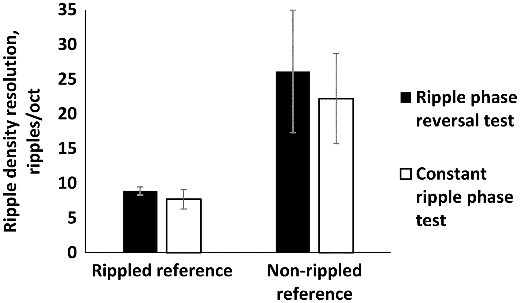

The test stimuli with constant ripple phases (see Figure 1(b)) in conjunction with rippled reference stimuli with ripple phase opposite to the test (see Figure 1(c)) resulted in a somewhat lower resolution of 7.7 ripples/oct, which is close to that obtained by Milekhina et al. (2018). Interindividual standard deviations for these estimates were 0.6 and 1.4 ripples/oct, respectively. The difference in 1.2 ripples/oct between these two estimates was not statistically significant (t = 1.83, df = 7, p = .11 by paired t test) which may be a result of the small group of listeners. In another study (Milekhina et al., 2018), the similar difference was statistically significant.

Measurements with nonrippled reference stimuli (see Figure 1(d)) resulted in much higher resolutions. For test stimuli with ripple-phase reversals (cf. Figure 1(a) and (d)), the mean resolution was 26.1 ripples/oct. For test stimuli with constant-phase ripples (cf. Figure 1(b) and (d)), the resolution was 21.2 ripples/oct. Interindividual standard deviations for these estimates were 8.9 and 6.5 ripple/oct, respectively. The difference in 4.9 ripples/oct between these two estimates was not statistically significant either (p = .41).

Thus, a pronounced result of the measurements was that the estimates of the ripple-density resolution obtained with the nonrippled reference stimulus were several times as high as those obtained with the rippled reference stimuli. For test stimuli with ripple-phase reversals, the difference in 17.2 ripples/oct between the results obtained with the different reference stimuli was highly statistically significant (t = 4.75, df = 5, p = .005). For the test stimulus with constant ripple phases, the difference in 14.5 ripples/oct between the results obtained with different reference stimuli was also highly statistically significant (t = 5.31, df = 5, p = .003).

Discussion

Result Summary

The data presented earlier show that estimates of the ripple-pattern resolution depend on the discrimination task, specifically on the type of the test and reference stimuli for the discrimination. Two regularities were noticed: (a) Test stimuli with ripple-phase reversals provided moderately higher resolution estimates compared with test stimuli with a constant ripple phase. This difference was noticed as a tendency that did not reach statistical significance. (b) Nonrippled reference stimuli provided much (several times) higher resolution estimates than rippled reference stimuli. This difference was highly statistically significant.

Comparison of Phase-Varying and Constant-Phase Test Stimuli

The difference between the results obtained with phase-varying and constant-phase test stimuli obtained in this study did not reach statistical significance; however, it could be considered to be a tendency. A similar difference (statistically significant) was described previously, and it has been hypothesized that the difference between the two test stimulus types appeared due to a greater involvement of cognitive processes (short-term memory) in the case of the constant-phase test stimuli (Milekhina et al., 2018). With the phase-varying test stimuli, phase changes could be detected directly as transients between segments with opposite ripple phases, whereas with the constant-phase test stimulus, a current stimulus (test or reference) is compared with a stimulus presented several seconds earlier, which requires the participation of short-term memory. This additional requirement could make the discrimination more difficult.

Comparison of Rippled and Nonrippled Reference Stimuli

Much more prominent was the difference between the ripple-density resolution estimates obtained with different reference stimuli. The discrimination between the rippled test stimulus and nonrippled reference stimulus was possible at ripple densities several times as high as that between the rippled test and rippled reference stimuli. This result agrees with data by Anderson et al. (2012) who measured ripple depth thresholds (the ripple detection task) using nonrippled reference stimuli: Ripple-depth thresholds were measurable at ripple densities several times higher than the ripple resolution found using ripped reference stimuli. We hypothesize that this difference can be explained by different roles of two basic mechanisms that underlie the ripple-pattern discrimination: the excitation-pattern mechanism and the temporal-processing mechanism.

The excitation-pattern model assumes that within the auditory system, an excitation pattern (an excitation-vs-frequency function) appears as the input signal passes through a bank of frequency-tuned filters (Zwicker, 1970). Because of the across-frequency integration within the filter bands, the ripple depth in the excitation pattern is reduced compared with the input signal. The changes in the ripple phase are detectable when the ripple depth in the excitation pattern exceeds a certain threshold.

Alternatively, the temporal-processing model implies an analysis of the temporal structure of the input signal. Rippled-spectrum signals are a type of noise and do not feature an obvious temporal structure; however, they have a hidden temporal structure that manifests in the autocorrelation function (ACF). ACF presents the interrelation of a function with its delayed copies. ACF of a rippled-spectrum signal features a peak at a lag of 1/δf, where δf is the ripple frequency spacing. This delayed ACF peak allows the discrimination of rippled and nonrippled signals, and the lag limit for ACF computation determines the ripple-density resolution. Involvement of temporal cues in rippled-spectrum signal processing has been demonstrated, mostly for wideband rippled noise with constant ripple spacing (Bilsen & Ritsma, 1970; Krumbholz, Patterson, & Nobbe, 2001; Patterson, Handel, Yost, & Datta, 1996; Yost, 1996; Yost et al., 1996). Next, the applicability of both the excitation-pattern and the temporal-processing models to the experimental data presented earlier is considered.

Excitation-Pattern Model

Figure 3(a) presents the rippled spectra with opposite ripple phases (1 and 2) and a nonrippled spectrum (3), and Figure 3(b) presents the simulations of excitation patterns produced by these signals (1–3, respectively). The ripple density is taken of 8 ripples/oct, which is close to the experimentally observed resolution limit. The two spectra of opposite ripple phase model either two alternative spectra of the test stimulus with ripple phase reversals or constant-phase test and rippled reference stimuli with opposite ripple phases. Excitation patterns were computed as a result of transferring the input spectra through a bank of filters described by a roex function (Patterson, Nimmo-Smith, Weber, & Milory, 1982) with an equivalent rectangular bandwidth of 0.12 of the center frequency (Glasberg & Moore, 1990), which corresponds to 0.17 oct. Due to integration within the filter passband, the excitation patterns have reduced ripple depth compared with the input signals (the higher the ripple density, the lower the ripple depth). At a ripple density of 8 ripples/oct, the maximal ripple depth (the ratio of a ripple peak to the nearest ripple trough) in the excitation pattern is 0.7 dB (Figure 3(b), 1 and 2). This depth is close to thresholds for excitation patterns produced by rippled stimuli (Green, 1983; Supin et al., 1999). The model assumes that the discrimination of patterns with opposite ripple phases is possible as long as the ripple depth exceeds a threshold for ripple detection. If the ripple depth is below the threshold (the ripples are not detectable), the rippled excitation patterns (Figure 3(b), 1 and 2) reduce to a nonrippled pattern. These patterns are not distinguishable from one another and from the truly nonrippled pattern (Figure 3(b), 3). Thus, the model predicts equal ripple-density resolution estimates for the discrimination both between rippled stimuli and between rippled and nonrippled stimuli. This prediction does not fit the experimental data. Quantitatively, the model does not fit the data obtain with nonrippled stimuli either. At a ripple density of 26 ripples/oct (which is the resolution with nonrippled reference stimuli), the maximal ripple depth in the computed excitation pattern is as low as 0.01 dB, which is well below the ripple depth threshold.

Figure 3.

Modeling of excitation-pattern analysis of rippled and nonrippled signals. (a) Input signal spectra (log frequency scale). (b) Excitation pattern computed by transferring the signals through a roex filter of 0.17-oct equivalent rectangular bandwidth. 1 and 2—rippled signals with opposite ripple phases and 3—nonrippled signal. The vertical dashed lines mark the central signal frequency of 2 kHz and show opposite ripple phases in 1 and 2.

Thus, the excitation-pattern model does explain the discrimination between rippled-spectrum stimuli with opposite ripple phases but not explain the discrimination between rippled and nonrippled stimuli.

Temporal-Processing Model

Band-pass signals with frequency-proportional ripple spacing (Figure 4(a), 1 and 2) have an ACF structure (Figure 4(b), 1 and 2) that contains an early segment and a delayed segment with a delay of τ = 1/δf, where δf is the ripple spacing. The delayed segment consists of waves of frequencies from f_min to f_max, where f_min and f_max are the lower and upper edges of the signal frequency band, respectively. The ACF is quite different for nonrippled reference signals (Figure 4(a), 3). It features no delayed segment.

Figure 4.

Modeling of temporal-processing analysis of rippled and nonrippled signals. (a) Input signal spectra (linear frequency scale). (b) ACF of the signals. 1 and 2—rippled signals with opposite ripple phases and 3—nonrippled signal. In panel (a), the vertical dashed lines mark the central signal frequency of 2 kHz and show opposite ripple phases in 1 and 2; in panel (b), 1—ACF waveform and 2—ACF envelope; the vertical dashed line marks the lag of 1/f₀ (f₀ is the central signal frequency of 2 kHz) and shows the opposite wave phases in 1 and 2. ACF = autocorrelation function.

Potentially, the differences both between the ACFs of two rippled-spectrum signals (1 and 2 in Figure 4(b)) and between the ACFs of the rippled and nonrippled signals (1 and 3 in Figure 4(b)) could provide a cue for the discrimination of these signals from one another, even at high ripple densities. With this discrimination mechanism, a ripple-density resolution limit appears when the delayed segment of the rippled-spectrum signal’s ACF shifts beyond the lag at which the ACF can be determined by the auditory system. At a 2-kHz center frequency, the found ripple-density resolution of 25 to 26 ripples/oct corresponds to approximately 17 to 18 ripples/kHz, thus indicating the lag limit of 17 to 18 ms.

If the discrimination were possible both between opposite-phase rippled signals and between a rippled and nonrippled signal, this limit should be equal for both these cases. This prediction contradicts the experimental data: The use of nonrippled reference stimuli resulted in much higher resolution than the use of rippled reference stimuli. Therefore, the ACF-based model may explain the experimental data under conditions of certain limitations. As such a limitation, it might be hypothesized that for the ACF discrimination, the temporal-processing mechanism exploits not the waveform within the delayed segment but a cue associated with the presence or absence of this segment. A possible (but not the only) cue might be the ACF envelope. It coincides for ACFs 1 and 2 in Figure 4(b) and differs for ACFs 1 and 3.

Thus, contribution of the temporal-processing mechanism might afford the discrimination between rippled and nonrippled stimuli at high ripple densities. However, this explanation is valid with an arbitrary assumption, which needs to be verified by further investigations. Therewith, the temporal-processing mechanism is expected to be ineffective for the discrimination between two rippled-spectrum stimuli.

Conclusion

Based on the considered models, it can be hypothesized that for processing of rippled-spectrum stimuli, the excitation-pattern and temporal-processing mechanisms are involved depending on the discrimination task, with the use of whatever cues are available. For the discrimination of a rippled test from a rippled reference stimulus, the excitation-pattern mechanism is more effective. For the discrimination of a rippled test stimulus from a nonrippled reference stimulus, the temporal-processing mechanism is effective. Hypothetically, different discrimination paradigms can be used for evaluation of the efficiency of the excitation-pattern and temporal-processing mechanisms.

Footnotes

Acknowledgments

The authors thank American Journal Experts for English language editing.

Declaration of Conflicting Interests

The authors declared no potential conflicts of interest with respect to the research, authorship, and/or publication of this article.

Funding

The authors disclosed receipt of the following financial support for the research, authorship, and/or publication of this article: The study was supported by the Russian Science Foundation, Grant 16-15-10046 and Russian Foundation for Basic Research, Grant 17-04-00096 to A. Y. S.

References

Anderson

E. S.

Nelson

D. A.

Kreft

Nelson

P. B.

Oxenham

A. J.

(2011) Comparing spatial tuning curves, spectral ripple resolution, and speech perception in cochlear implant users. Journal of the Acoustical Society of America 130: 364–375. DOI: 10.1121/1.3589255.

Anderson

E. S.

Oxenham

A. J.

Nelson

P. B.

Nelson

D. A.

(2012) Assessing the role of spectral and intensity cues in spectral ripple detection and discrimination on cochlear-implant users. Journal of the Acoustical Society of America 132: 3925–3934. DOI: 10.1121/1.4763999.

Aronoff

J. M.

Landsberger

D. M.

(2013) The development of a modified spectral ripple test. Journal of the Acoustical Society of America 134: EL217–EL222. DOI 10.1121/1.4813802.

Azadpour

McKay

C. M.

(2012) A psychophysical method for measuring spatial resolution in cochlear implants. Journal of the Association for Research in Otolaryngology 13: 145–157. DOI: 10.1007/s10162-011-0294-z.

Bilsen

F. A.

Ritsma

R. J.

(1970) Some parameters influencing the perceptibility of pitch. Journal of the Acoustical Society of America 47: 469–475. DOI: 10.1121/1.1911916.

Chi

Gao

Guyton

M. G.

Shamma

(1999) Spectro-temporal modulation transfer function and speech intelligibility. Journal of the Acoustical Society of America 106: 2719–2732. DOI: 10.1121/1.428100.

Glasberg

B. R.

Moore

B. C. J.

(1990) Derivation of auditory filter shapes from notched-noise data. Hearing Research 47: 103–138. DOI: 10.1016/0378-5955(90)90170-T.

Green

D. M.

(1983) Profile analysis: A different view of auditory intensity discrimination. American Psychologist 38: 133–142.

Henry

B. A.

Turner

C. W.

Behrens

(2005) Spectral peak resolution and speech recognition in quiet: Normal hearing, hearing impaired, and cochlear implant listeners. Journal of the Acoustical Society of America 118: 1111–1121. DOI: 10.1121/1.1944567.

10.

Jeon

E. K.

Turner

C. W.

Karsten

S. A.

Henry

B. A.

Gantz

B. J.

(2015) Cochlear implant users’ spectral ripple resolution. Journal of the Acoustical Society of America 138: 2350–2358. DOI: 10.1121/1.4932020.

11.

Krumbholz

Patterson

R. D.

Nobbe

(2001) Asymmetry of masking between noise and iterated rippled noise: Evidence for time interval processing in the auditory system. Journal of the Acoustical Society of America 110: 2096–2107. DOI: 10.1121/1.1395583.

12.

Levitt

(1971) Transformed up-down methods in psychoacoustics. Journal of the Acoustical Society of America 49: 467–477. DOI: 10.1121/1.1912375.

13.

Litvak

L. M.

Spahr

A. J.

Saoji

A. A.

Fridman

G. Y.

(2007) Relationship between perception of spectral ripple and speech recognition in cochlear implant and vocoder listeners. Journal of the Acoustical Society of America 122: 982–991. DOI: 10.1121/1.2749413.

14.

Milekhina

O. N.

Nechaev

D. I.

Supin

A. Y.

(2018) Estimates of frequency resolving power of humans by different methods: The role of sensory and cognitive factors. Human Physiology 44: 357–363.

15.

Narne

V. K.

Sharma, M., Van Dun

Bansal

Prabhu

Moore

B. C. J.

(2016) Effects of spectral smearing on performance of the spectral ripple and spectro-temporal ripple tests. Journal of the Acoustical Society of America 140: 4298–4306. DOI: 10.1121/1.4971419.

16.

Nechaev

D. I.

Milekhina

O. N.

Supin

A. Y.

(2018) Hearing sensitivity to gliding rippled spectrum patterns. Journal of the Acoustical Society of America 143: 2387–2393. DOI: 10.1121/1.5033898.

17.

Nechaev

D. I.

Supin

A. Y.

(2013) Hearing sensitivity to shifts of rippled-spectrum patterns. Journal of the Acoustical Society of America 134: 2913–2922. DOI: 10.1121/1.4820789.

18.

Patterson

R. D.

Handel

Yost

W. A.

Datta

A. J.

(1996) The relative strength of the tone and noise components in iterated rippled noise. Journal of the Acoustical Society of America 100: 3286–3294. DOI: 10.1121/1.417212.

19.

Patterson

R. D.

Nimmo-Smith

Weber

D. L.

Milory

(1982) The deterioration of hearing with age: Frequency selectivity, the critical ratio, the audiogram, and speech threshold. Journal of the Acoustical Society of America 72: 1788–1803. DOI: 10.1121/1.388652.

20.

Saoji

A. A.

Litvak

Spahr

A. J.

Eddins

D. A.

(2009) Spectral modulation detection and vowel and consonant identification in cochlear implant listeners. Journal of the Acoustical Society of America 126: 955–958. DOI: 10.1121/1.3179670.

21.

Supin

A. Y.

Popov

V. V.

Milekhina

O. N.

Tarakanov

M. B.

(1994) Frequency resolving power measured by rippled noise. Hearing Research 78: 31–40. DOI: 10.1016/0378-5955(94)90041-8.

22.

Supin

A. Y.

Popov

V. V.

Milekhina

O. N.

Tarakanov

M. B.

(1997) Frequency-temporal resolution of hearing measured by rippled noise. Hearing Research 108: 17–27. DOI: 10.1016/S0378-5955(97)00035-X.

23.

Supin

A. Y.

Popov

V. V.

Milekhina

O. N.

Tarakanov

M. B.

(1998) Frequency resolving power at various rippled-noise patterns. Journal of the Acoustical Society of America 103: 2042–2050. DOI: 10.1121/1.421351.

24.

Supin

A. Y.

Popov

V. V.

Milekhina

O. N.

Tarakanov

M. B.

(1999) Ripple depth and density resolution in rippled noise. Journal of the Acoustical Society of America 106: 2800–2804. DOI: 10.1121/1.428105.

25.

Supin

A. Y.

Popov

V. V.

Milekhina

O. N.

Tarakanov

M. B.

(2003) Rippled-spectrum resolution dependence on level. Hearing Research 185: 1–12. DOI: 10.1016/S0378-5955(03)00215-6.

26.

Supin

A. Y.

Popov

V. V.

Milekhina

O. N.

Tarakanov

M. B.

(2010) Masking of rippled-spectrum-pattern resolution in diotic and dichotic presentations. Hearing Research 260: 109–116. DOI: 10.1016/j.heares.2009.12.018.

27.

van Zanten

G. A.

Senten

C. J. J.

(1983) Spectro-temporal modulation transfer function (STMTF) for various types of temporal modulation and a peak distance of 200 Hz. Journal of the Acoustical Society of America 74: 52–62. DOI: 10.1121/1.389617.

28.

Won

J. H.

Drennan

W. R.

Rubinstein

J. T.

(2007) Spectral-ripple resolution correlates with speech reception in noise in cochlear implant users. Journal of the Association for Research in Otolaryngology 8: 384–392. DOI: 10.1007/s10162-007-0085-8.

29.

Won

J. H.

Humphrey

E. L.

Yeager

K. R.

Martinez

A. A.

Robinson

C. H.

Mills

K. E.

Woo

(2014) Relationship among the physiologic channel interactions, spectral-ripple discrimination, and vowel identification in cochlear implant users. Journal of the Acoustical Society of America 136: 2714–2725. DOI: 10.1121/1.4895702.

30.

Yost

W. A.

(1996) Pitch strength of iterated rippled noise. Journal of the Acoustical Society of America 100: 3329–3335. DOI: 10.1121/1.416973.

31.

Yost

W. A.

Hill

(1978) Strength of the pitches associated with ripple noise. Journal of the Acoustical Society of America 64: 485–492. DOI: 10.1121/1.382021.

32.

Yost

W. A.

Hill

Perez-Falcon

(1978) Pitch and pitch discrimination of broadband signals with rippled power spectra. Journal of the Acoustical Society of America 63: 1166–1173. DOI: 10.1121/1.381824.

33.

Yost

W. A.

Patterson

R. D.

Sheft

(1996) A time domain description for the pitch strength of iterated rippled noise. Journal of the Acoustical Society of America 99: 1066–1078. DOI: 10.1121/1.414593.

34.

Zwicker

(1970) Masking and psychophysical excitation as consequences of the ear’s frequency analysis. In: Plomp

Smoorenburg

G. F.

(eds) Frequency analysis and periodicity detection in hearing, Leiden, the Netherlands: Sijthoff, pp. 376–394.

Estimates of Ripple-Density Resolution Based on the Discrimination From Rippled and Nonrippled Reference Signals

Abstract

Keywords

Introduction

Materials and Methods

Listeners

Stimuli

Stimulus Generation

Experimental Procedure

Instrumentation

Results

Discussion

Result Summary

Comparison of Phase-Varying and Constant-Phase Test Stimuli

Comparison of Rippled and Nonrippled Reference Stimuli

Excitation-Pattern Model

Temporal-Processing Model

Conclusion

Footnotes

Acknowledgments

Declaration of Conflicting Interests

Funding

References