Sage Journals: Discover world-class research

Abstract

Most hearing aid prescriptions focus on the optimization of a metric derived from the long-term average spectrum of speech, and do not consider how the prescribed values might distort the temporal envelope shape. A growing body of evidence suggests that such distortions can lead to systematic errors in speech perception, and therefore hearing aid prescriptions might benefit by including preservation of the temporal envelope shape in their rationale. To begin to explore this possibility, we designed a genetic algorithm (GA) to find the multiband compression settings that preserve the shape of the original temporal envelope while placing that envelope in the listener’s audiometric dynamic range. The resulting prescription had a low compression threshold, short attack and release times, and a combination of compression ratio and gain that placed the output signal within the listener’s audiometric dynamic range. Initial behavioral tests of individuals with impaired hearing revealed no difference in speech-in-noise perception between the GA and the NAL-NL2 prescription. However, gap detection performance was superior with the GA in comparison to NAL-NL2. Overall, this work is a proof of concept that consideration of temporal envelope distortions can be incorporated into hearing aid prescriptions.

Keywords

compression temporal processing genetic algorithms optimization

Introduction

Advances in hearing aid technology have led to a dramatic increase in the number of signal processing parameters that influence the behavior of the device. It is common for a hearing aid to have well over 100 continuous parameters, making the space of potential parameter combinations far too large to explore comprehensively. To deal with this problem, in most clinical applications parameter values are determined by prescriptive formulas that are designed to optimize the perception of speech according to a theoretically driven rationale.

The rationales underlying the most common prescriptive formulae (e.g., NAL-NL2; Keidser, Dillon, Flax, Ching, & Brewer, 2011; and DSL v5.0; Scollie et al., 2005) are designed to optimize an acoustical index that is derived from the long-term average spectrum of speech. For example, the commonly used prescriptions from the National Acoustics Laboratory (Byrne, Dillon, Ching, Katsch, & Keidser, 2001; Keidser et al., 2011) are designed to satisfy two major constraints. First, these prescriptions find the parameter values that optimize the speech intelligibility index (SII; ANSI, 1997). The SII is a metric that reflects the audibility of the long-term average speech spectrum, such that frequency ranges that are critical for speech are weighted more heavily than ranges that are less important. Second, the prescribed gain values are constrained by a model of loudness growth that was designed for hearing-impaired ears (e.g., Moore & Glasberg, 2004) so that the perceived loudness in the hearing aid wearer does not exceed that in a listener with normal hearing given the same input. The desired sensation-level prescriptions (Cornelisse, Seewald, & Jamieson, 1995; Scollie et al., 2005) are primarily designed to optimize the audibility of the long-term average spectrum of speech without exceeding the patient’s uncomfortable listening level (UCL). In the nonlinear versions of these prescriptions, these constraints are evaluated at numerous input levels so that gain is prescribed as a function of both frequency and input level. The primary acoustical information considered for both formulas is the long-term average spectrum of speech for a variety of sound levels. Thus, prescriptions do not consider the relatively slow (2–50 Hz) fluctuations in sound level over time, referred to here as the temporal envelope. It might be important to consider such fluctuations because, in addition to the spectral envelope, the temporal envelope carries a great deal of linguistic information about features such as consonant manner and voicing as well as prosodic cues (for review see Rosen, 1992).

Given the importance of the temporal envelope to hearing, it might be important to consider how the parameter values comprising the hearing aid prescription influence the shape of that envelope. In particular, it is well known that the shape of the natural temporal envelope can be dramatically altered by the use of wide dynamic range compression (WDRC; for review see Souza, 2002). WDRC is a signal processing technique used in nearly all modern hearing aids that reduces the dynamic range of the signal to accommodate the reduced audiometric dynamic range in the impaired auditory system (Moore, Glasberg, Hess, & Birchall, 1985). For example, WDRC can reduce the depth of amplitude fluctuations (amplitude modulation) in the temporal envelope, distorting the envelope shape (Stone & Moore, 1992, 2007), and can reduce the signal-to-noise ratio (Naylor & Johannesson, 2009; Souza, Jenstad, & Boike, 2006). The extent to which WDRC distorts the envelope is dependent on the specific parameter values used such as whether the compression has fast or slow time constants (Moore, 2008). These distortions to the temporal envelope might lead to reductions in speech perception and sound quality (e.g., Drullman, Festen, & Plomp, 1994; Kates, 2010; Payton & Braida, 1999). Relevant to the current work, Souza and Gallun (2010) demonstrated a link between errors in consonant identification and distortions of the temporal envelope that were introduced by hearing aid signal processing. Specifically, the number of errors increased as the correlation between the envelopes of the unmodified and hearing aid–processed signals decreased. Further, when errors did occur, the type of confusion was consistent with the idea that the listener was choosing the token whose unmodified temporal envelope was most similar to the hearing aid-modified envelope. Taken together, there is considerable evidence that the shape of the temporal envelope is among the acoustical cues that contribute to accurate speech perception, and that cue can be distorted by some implementations of compression. Therefore, it is possible that hearing aid prescriptions might benefit from including preservation of the temporal envelope shape in the underlying rationales.

In this article, we explore the development and evaluation of a prescription that focuses on preserving the shape of the temporal envelope. The goal here is not to develop a new prescription per se but rather to describe a method for incorporating temporal envelope preservation into the development of a hearing aid prescription, to explore which parameter values result from this development, and to examine the perceptual consequences of those values on tasks thought to depend on temporal perception.

This work centers on the use of an optimization technique known as a genetic algorithm (GA) to find the parameter values that preserve temporal envelope shape. GAs are inspired by the process of natural selection and can efficiently explore expansive ranges of parameter settings with minimal assumptions. Briefly, an initial population of genes (each gene is an array of values) is created and ranked according to a measure of fitness that is tailored to the underlying rationale. Only the genes with relatively high fitness survive to the next generation (Figure 1a). The rest of the new generation is filled through mating (combining the values of the high-fitness genes, Figure 1b and mutation (randomly adjusting parameter values of the high-fitness genes, Figure 1c). This process is iterated over time, and the maximum fitness increases across generations. Ultimately some stopping criterion is reached, and the gene with the highest fitness in the newest generation is taken as the optimal solution.

Figure 1.

Genetic algorithm. In a genetic algorithm, each gene is an array of values. The values in each gene change over generations to maximize a fitness function. A new generation is created through (a) preservation: maintaining the values of the previously high-fitness genes, (b) mating: randomly combining values from high-fitness genes, and (c) mutation: randomly altering some values in high-fitness genes.

In several auditory investigations, researchers have combined GAs and behavior to find the setting that was preferred by the listener. In these cases, the fitness of a gene was determined by a behavioral response from a listener. For example, GAs have been used to set parameters of a cochlear implant speech processor (Wakefield, van den Honert, Parkinson, & Lineaweaver, 2005), a speech vocoder (Baskent, Eiler, & Edwards, 2007), a hearing aid feedback reducer (Durant, Wakefield, Van Tasell, & Rickert, 2004), and in the selection of individualized direction transfer functions (Durant & Wakefield, 2002). In those experiments, the GA repeatedly converged on an optimal solution in a relatively small number of generations (e.g., ∼10). However, in each of those experiments, the number of parameters was restricted (usually three to four in total), as was the range of potential values that the parameters could take. Even with those restrictions, this procedure was too long to be clinically feasible (usually at least 1 hr). A subjective-preference-based GA would likely be made considerably longer if expanded to include the larger number of parameters that are necessary to control a multiband compressor.

Instead, we use a GA to find the parameter values that optimize an acoustical, rather than behavioral, measure of the signal. Using an acoustically derived fitness function frees us from the time constraints of behavioral testing and allows a more comprehensive exploration of the parameter space. Specifically, following Souza and Gallun (2010), we attempt to find the parameter values that optimize the correlation between the unmodified and hearing aid–modified temporal envelopes while providing a frequency–gain function that is appropriate to place the envelope in the listener’s audiometric dynamic range.

We also report results of an initial exploration into the behavioral consequences of this new fit. We focus on two tasks known to depend on temporal envelope perception. Specifically, we focus on speech perception in background babble (Killion, Niquette, Gudmundsen, Revit, & Banerjee, 2004), because the accurate perception of the target speech might require listeners to focus on the dips of the temporal envelope of the background babble. We also measure performance on gap detection, a task that is often used as an overall measurement of temporal processing ability.

Experiment I: Algorithm Analysis

In this experiment, we ran the GA for several test audiograms and examined the electro-acoustical characteristics of the resulting fits.

Method

Multiband compression

WDRC was implemented using the custom-written six-channel multiband compressor described in the following.

Filtering

Each of the six channels was passed through a bandpass filter before and after compression. Each filter was a fourth-order Butterworth bandpass filter with an octave-wide bandwidth and center frequencies in octave steps from 250 to 8000 Hz (as in Gallun & Souza, 2008; Souza & Gallun, 2010).

Compression

Compression was applied offline using a custom-written algorithm. The compressor had five adjustable parameters: threshold, ratio, attack time constant, release time constant, and gain.

All operations were performed on the temporal envelope (env), which was first extracted by computing the root-mean-square amplitude (in dB) with a 10-ms moving rectangular window ending with the current sample (the ith sample). This envelope was subsequently smoothed according to the attack and release time constants, as described later. The gain control signal was dependent on the temporal envelope input level (env, in dB SPL), the gain (Gain, in dB), the compression threshold (Thr, in dB SPL), and the ratio (Ratio, in dB/dB) according to the piecewise function described in Equation 1:

Gain + {\frac{1 - Ratio}{Ratio} ({env}_{i} - Thr) if {env}_{i} > Thr 0 otherwise .

(1)

The input signal was delayed by 10 ms relative to the gain control signal. By applying a small delay of the signal relative to the gain control signal, the level of transient increases in the sound level can be reduced.

Before Equation 1 was applied, the temporal envelope was smoothed using the single-pole low-pass filter (IIR) described in Equation 2:

{env}_{i} = (1 - Θ) {rms}_{i} + Θ {env}_{i - 1}

(2)

where rms is the temporal envelope extracted with the 10-ms moving rectangular window and env is the smoothed temporal envelope. Note that the time constant Θ controls the influence of the previous smoothed envelope value on the current one. For instance, if Θ = 0, then env is identical to rms. As Θ increases, the influence of a given envelope value remains for a longer period, and thus more smoothing occurs.

Separate values of Θ were applied depending on whether the temporal envelope was increasing (in attack) or decreasing (in release) according to Equation 3:

Θ \equiv {e^{- 1 / (F_{s} Att)} if {rms}_{i} > {env}_{i} e^{- 1 / (F_{s} Rel)} otherwise,

(3)

where Att and Rel are the attack and release time constants and Fs is the sampling rate (in Hz).

We note that Att and Rel are not equivalent to the attack and release times as defined by ANSI (2003). To report values consistent with ANSI specification, the attack and release times reported here were computed empirically. Specifically, the attack time was defined as the time it takes the output to drop to within 3 dB of the steady-state level after a 2000-Hz sinusoidal input changes from 55 dB SPL to 90 dB SPL. Release time was defined as the time it takes the 2000-Hz sinusoidal output to stabilize to within 4 dB of the steady-state level after input changes from 90 dB SPL.

Summation

Finally, after filtering and compression, the six channels were summed together and taken as the output.

Genetic Algorithm

Overview

We designed the GA to select the multiband compressor parameters that placed the temporal envelope within a simulated listener’s audiometric dynamic range while preserving the unmodified envelope shape.

The GA was run separately for each band, and thus did not take into account any across-band interactions that may occur due to overlapping filter frequency responses. In this algorithm, each gene was a set of parameter values for a band-specific compressor. Initially, a population of 100 random genes was created (see the Initialization), and the fitness of each gene was evaluated (see the Evaluation of Fitness section). Only the genes with the highest fitness from that generation survived the next generation. The remaining positions in the new generation were filled by a combination of mating and mutating the genes from the current generation (see the Determination of Next Generation section). This process was repeated for several generations until a stopping criterion was reached (see the Stopping Criterion section). If the audiometric threshold at a particular frequency was less than 20 dB HL or greater than 90 dB HL, we did not run the GA.

Test audiograms

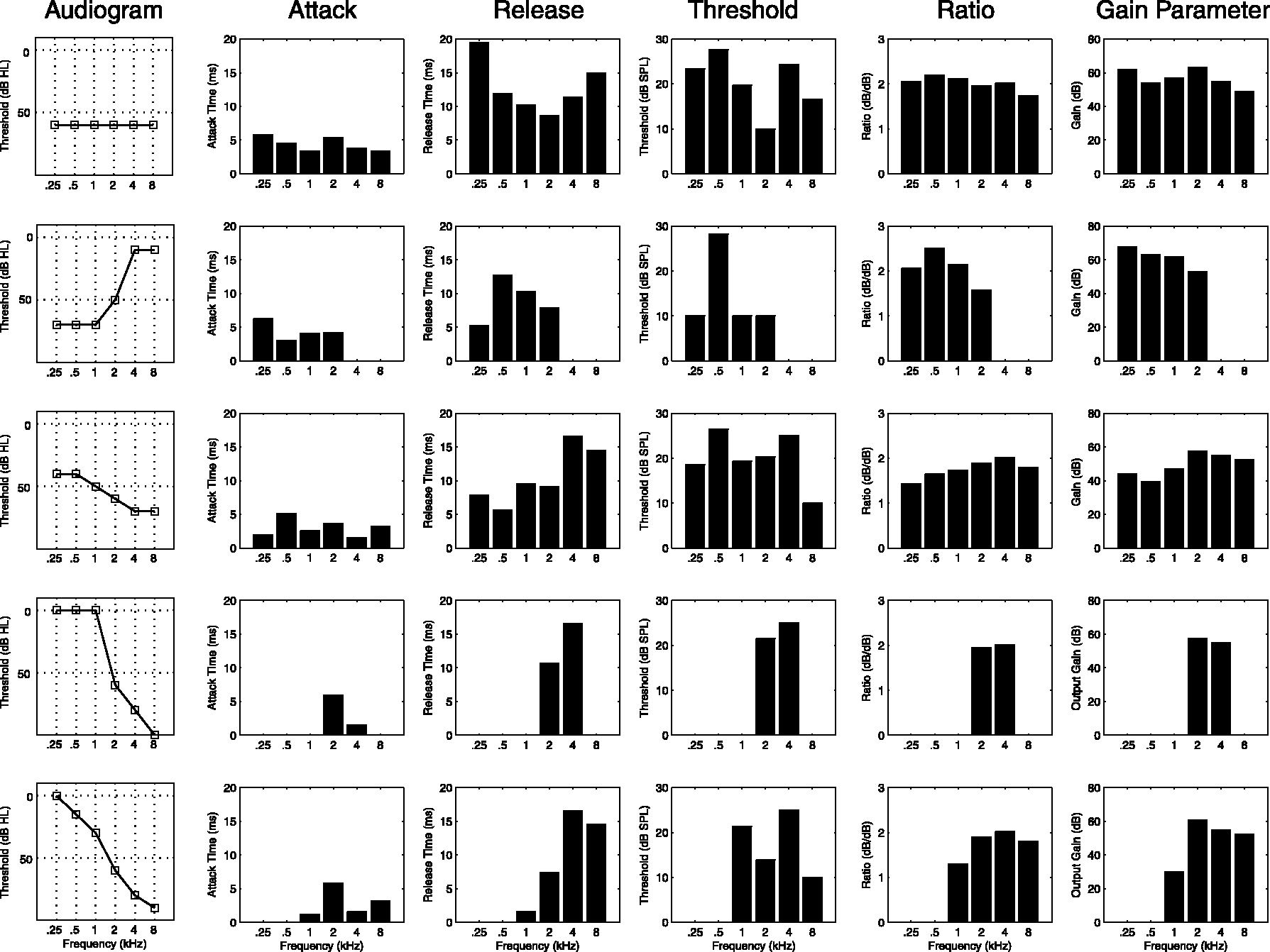
The GA optimization was run for each of the five simulated audiograms displayed in the left column of Figure 4 (the same audiograms as in Byrne et al., 2001, their Figure 2). This set of audiograms contains a flat loss (row 1), a reverse-sloping loss (row 2), and three variations of sloping losses (rows 3–5). In Experiment II, described later, prescriptions were created based on each listener’s audiogram.

Figure 2.

Fitness computation. In each generation of the genetic algorithm, each gene was given a fitness score. To do so, we computed the temporal envelope of the (a) unmodified and (b) compressed envelopes. We then (c) modified the compressed envelope to take into account the listener’s hearing abilities. Specifically, we performed notch clipping at the audiometric threshold and peak reflection at the uncomfortable listening level. The fitness value was the Pearson correlation between the modified compressed envelope (c) and the unmodified envelope (a).

Figure 4.

Genetic algorithm (GA)-prescribed multiband compression values. The genetic algorithm was run on five different audiograms (left column). The band-specific values (bars in each plot) are plotted separately for each compression parameter (remaining columns). Overall, the GA prescribed fast attack and release time constants and low compression thresholds. The ratio and output gain values place the temporal envelope of the test signal into the listener’s audiometric dynamic range.

Test stimuli

The fitness of the GA was always assessed using a portion of the International Speech Test Signal (Holube, Fredelake, Vlaming, & Kollmeier, 2010). This signal was designed to capture relevant acoustical properties of natural speech (e.g., frequency and modulation spectra). The signal used for the optimization was 42 s in total, consisting of 21 s at 50 dB SPL followed by 21 s at 80 dB SPL.

Initialization

The first generation of 100 genes was created using random parameter values selected from predetermined ranges. Five channel-specific parameters were considered: threshold, ratio, attack time constant, release time constant, and gain. The threshold values were randomly selected from all integers ranging from 10 to 90 dB SPL. The gains were selected from integers ranging from 0 to 70 dB. The ratios were selected from continuous values ranging from 1:1 to 10:1. Finally, the attack and release time constant (Att and Rel, Equation 3) times were selected from a logarithmic distribution spanning 0.001 to 0.3. The measured time constants depend on the other parameters, but across the whole experiment spanned the attack times ranged from 1 to 357 ms, and the release time ranged from 1 to 929 ms.

Evaluation of fitness

The fitness criterion was designed to determine the parameter values that preserved the temporal envelope shape, while also providing a frequency–gain curve that was suprathreshold and below a simulated UCL. Our measure of fitness was related to the Pearson correlation coefficient between the unmodified (Figure 2a) and compressed temporal envelopes (Figure 2b). A high-envelope correlation coefficient meant that the compressor led to little distortion of the temporal envelope, and a low coefficient indicated a large amount of distortion. Note that this criterion does not ensure the best fit in terms of a measure such as speech intelligibility or quality. This criterion was simply chosen as a first step to demonstrate how a GA can minimize the temporal envelope distortions introduced by a hearing aid prescription.

Envelope extraction was accomplished by half-wave rectification, followed by 50-Hz low-pass filtering (Gallun & Souza, 2008; Souza & Gallun, 2010). Before computing the envelope correlation, we performed two manipulations on the compressed temporal envelope. To account for the amount of hearing loss at a given frequency, we notch clipped the temporal envelope at the audiometric threshold for a pure tone at the center of the pass-band (Figure 2c). Envelope values lower than the audiometric threshold were replaced with the threshold value. This step penalized the fitness value of genes that made the signal subthreshold. We also penalized genes that placed the signal above the UCL. We first used the formula applied to the audiometric threshold described in Dillon and Storey (1998) to estimate UCL and then corrected for the difference between speech peaks and average level (Cox, Matesich, & Moore, 1988). We initially tried to peak-clip the compressed envelope at the UCL. However, initial investigations indicated that the overall effect of this manipulation on the uncompressed versus compressed envelope correlation was minimal, and the resulting fits often had temporal envelopes that exceeded the UCL. Therefore, to increase the penalty for exceeding the UCL on the correlation we reflected peaks that exceeded the UCL. For example, if the UCL was 100 dB SPL, and the compressed envelope had a value of 110 dB SPL, we instead set that value to 90 dB SPL. Since this manipulation inverted the relationship between the input and the output, the effect of exceeding the UCL on the correlation coefficient was more dramatic. After notch clipping and peak reflection, we computed the Pearson correlation coefficient between the unmodified (Figure 2a) and the modified compressed amplitude envelopes (Figure 2c). The resulting value was taken as our measure of fitness. This measure is a modification of the correlation-based metric for comparing envelopes proposed by Gallun and Souza (Gallun & Souza, 2008; Souza & Gallun, 2010).

Determination of next generation

Each subsequent generation was determined by taking the top genes from the previous generation, as well as by creating new genes by mating and mutating those top genes. After fitness was evaluated for an entire generation, the top 10 genes were preserved for the next generation (Figure 1a).

For the remaining 90 genes in the new generation, there was a 50% chance of that gene being created by mating (Figure 1b). If mating occurred, the two parents were selected randomly from the 10 genes that were preserved. The crossover points were determined randomly as well. We treated threshold, ratio, and gain as one unit, because their contributions to fitness are dependent on one another. Attack and release times were each treated separately. Therefore, there could be either one or two crossover points, creating three total mating possibilities. If mating did not occur, the new gene was identical to its parent until the mutation stage.

Mutation (Figure 1c) was accomplished by multiplying the values comprising the gene by random numbers. For each value in a gene, mutation occurred with 50% probability. If mutation occurred, the previous parameter value was multiplied by a random number drawn from a normal distribution with mean of 1 and standard deviation of 0.5.

Stopping criterion

Finally, we stopped the algorithm when we had inferred that it had converged on a final setting. When the maximum fitness of the current generation was within 0.002 of the previous 3 generations, the procedure was stopped. The gene with the maximum fitness in the final generation was taken as the winner.

Overall, the GA was designed so that the fitness increases over time. For example, in Figure 3, we have plotted the results of the GA optimization run for an example audiogram (Audiogram 1 in Figure 4, left column, top row). Notice that, for the plotted band, much of the uncompressed temporal envelope (Figure 3a) is inaudible. Audibility improves for the winner of the first generation (Figure 3b), though much of the speech envelope is still inaudible. By the final generation (Figure 3c), the entire speech envelope is audible and the peaks do not exceed the UCL. For this example optimization, we have also plotted, separately for each band, the fitness value of the best gene as a function of generation number (Figure 3d). Notice that the maximum fitness increases over multiple generations with the largest improvements occurring over the early generations. Each band has a different trajectory. In general, fewer generations are needed for bands where the initial fitness is high.

Figure 3.

Example optimization. (a) The unmodified temporal envelope in one example frequency band. The envelope of the same signal processed by the winning gene of the first (b) and final (c) generation. Note how audibility increases from the first to last generation, yet the relative shape of the final envelope matches that of the unmodified envelope. (d) Maximum fitness values as a function of generation, plotted separately for each band of an example audiogram. Note that fitness improves over generations with the largest improvements generally occurring in the earlier generations.

Results

Description

In all cases, the GA improved beyond the initial fitness. The median fitness value of the first generation was r = 0.88, and by the last generation it reached r = 0.93. The median number of generations to reach the stopping criterion was 18.

The parameter values of each of the winning genes are plotted for each of the example audiograms (rows) in Figure 4. We first note that for all audiograms the attack and release times (Figure 4, columns 2 and 3, respectively) were short. The median attack and release times were 6.1 and 10.7 ms, respectively. This attack time is within the normal range of fast time constants, but the release time is much shorter than what would normally be prescribed. The compressor threshold (Figure 4, column 4) was quite low and shows little variation across audiograms. The median threshold of (17.4 dB SPL) was quite close to the bottom of the dynamic range of speech. For each of these three parameters, there was no correlation between the assigned parameter value and the amount of hearing loss (all p > .08).

In contrast, the ratio and gain values (Figure 4, columns 5 and 6) were systematically related to the audiogram. We initially evaluated whether the GA-prescribed compression ratio would be related to the ratio between the dynamic range of speech and that of the simulated listener’s hearing. We considered this to be a logical starting point because the GA was designed to maximize the availability of the temporal envelope of speech within the audiometric dynamic range. The dynamic range of speech was estimated as the difference in dB between the 1st and 99th percentiles of the values of the envelope of the unmodified test signal, which comprised quiet and loud speech envelopes. The audiometric dynamic range was estimated as the difference in dB between the audiometric threshold and UCL. The relationship between these two ratios is plotted in Figure 5a and is captured by the linear equation displayed at the bottom right corner of the figure (r = 0.8, p < .001). There was a similarly straightforward relationship between audiometric threshold and the gain parameter resulting from this optimization (r = 0.86, p < .001). This relationship is plotted in Figure 5b and is captured by the linear equation at the bottom right corner.

Figure 5.

Analysis of genetic algorithm (GA)-prescribed values. Some values prescribed by the GA were predictable from the audiogram. (a) The compression ratio parameter value prescribed by the GA was linearly correlated with the band-specific ratio between the dynamic range of the test speech signal and the listener’s audiometric dynamic range. (b) The output gain parameter value prescribed by the GA for a given band was linearly correlated with the audiometric threshold for that band. (c) When we compute the target insertion gain using the values from the fitted lines (rather than the prescribed values) in conjunction with the median prescribed compression threshold, the resulting insertion gains are extremely close to those resulting from the GA-prescribed parameter values.

Taken together, the analyses described earlier can be summarized by a straightforward set of rules. The attack, release, and threshold parameters can all be set to the median value observed across all audiograms and bands. We use the across-group median here, because these parameters were not related to the audiogram. In contrast, ratio and gain are determined using the listener-specific audiometric thresholds and the linear functions described earlier.

For each audiogram and band, we can compute an insertion gain value by computing the level of a compressed signal and subtracting the level of the uncompressed signal. If we use this summary rule to compute insertion gains, for a pure-tone input of 50, 65, and 80 dB SPL input and compare them to the values obtained through the GA itself, there is a very close correspondence between the resulting gain values. This relationship is plotted in Figure 5c, where the correlation between the summary-rule-based and GA-based insertion gains is very high (r = 0.99, p < .001), and the average absolute value of the difference in dB is low (1.58 dB). Therefore, for the behavioral experiments described later, all multiband compression parameter values were determined using this rule (derived from the GA analysis) rather than running the GA separately for each patient.

Acoustical comparison to NAL-NL2

For each of the five example audiograms, we computed the target insertion gains (pure-tone input) as a function of frequency at input levels 50, 65, and 80 dB SPL for both the GA prescription (Figure 6, left column) and for NAL-NL2 (Figure 6, right column). NAL-NL2 was selected for comparison because it is the most commonly used nonlinear hearing aid prescription in the United States. Several dramatic differences between the two prescriptions can immediately be observed. In nearly all cases, the target insertion gain prescribed by the GA is higher than that of NAL-NL2. This gain difference is particularly large in the lower frequencies where, in some cases, the GA-optimized fit prescribes >30 dB more gain than NAL-NL2.

Figure 6.

Comparison of insertion gain between the genetic algorithm and NAL-NL2. Insertion gain is plotted as a function of frequency for each of the five audiograms in Figure 4. Gain values are plotted for a pure-tone input level of 50, 65, and 80 dB SPL (top, middle, and bottom lines, respectively). Note that in nearly all cases the genetic algorithm prescribes more insertion gain, especially at the lower frequencies.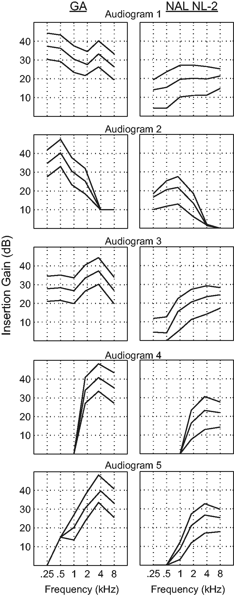

Overall, the GA prescribed a lower compression threshold and a less severe ratio than did NAL-NL2. In terms of compression threshold, the values prescribed by NAL-NL2 (50–52 dB SPL) are considerably higher than the median value obtained with the GA (17.4 dB SPL). The compression ratios prescribed by NAL-NL2 were slightly, but consistently, higher (median = 1.90) than those prescribed by the GA (median = 1.64, t₅₉ = −3.68, p < .001). Finally, no comparison between time constants can be made between the two prescriptions because NAL-NL2 does not prescribe time constants.

Experiment II: Behavioral Testing

In Experiment II, we performed an initial behavioral examination comparing some of the perceptual consequences of the GA-based prescription to those of with the NAL-NL2 prescription. For both prescriptions, we evaluated the performance of listeners with sensorineural hearing loss on tasks thought to depend on temporal perception.

Method

Participants

Ten listeners with mild-to-severe sensorineural hearing loss were recruited for the research project (summarized in Table 1). Normal middle ear function was confirmed through otoscopic screening, bone conduction testing (air-bone gaps no greater than 10 dB at octave frequencies < 8 kHz), and tympanometric values within normal ranges (Wiley et al., 1996). Nine of the listeners had symmetrical losses, as defined by between-ear threshold differences ≤20 dB at all tested frequencies between the two ears. The remaining listener (HI-024) was tested in her left ear, because the loss in her other ear was too severe to provide adequate amplification. For the other listeners, the test ear was determined randomly. Participants were recruited without regard for prior hearing aid usage. Three subjects were current hearing aid users, two were not current hearing aid users but had previously worn aids, and five had never worn hearing aids. All participants gave informed consent and were compensated for their time. All procedures were approved by the Institutional Review Board of Northwestern University.

Table 1.

Listener Demographics.

Subject	Tested ear	Gender	Age	Audiogram in tested ear (dB HL)
Subject	Tested ear	Gender	Age	250	500	1,000	2,000	4,000	8,000
HI-021	R	M	89	25	35	40	60	65	90
HI-013	L	M	82	35	45	50	70	80	75
HI-015	R	M	77	35	35	35	65	60	75
HI-026	R	F	79	35	25	35	50	45	65
HI-028	R	F	80	35	35	15	50	65	80
HI-024	L	F	85	35	25	20	45	50	50
HI-023	L	F	84	25	20	30	55	65	65
HI-031	L	F	79	45	45	45	45	55	70
HI-049	L	M	52	25	25	25	50	55	60
HI-030	R	M	62	15	20	15	25	55	60

Note: For each of the 10 subjects tested in this experiment, the tested ear, gender, age (in years), and audiogram of the tested ear are listed.

Equipment

Participants were seated in a double-walled sound-treated booth throughout the experiment and tasks were automated by custom-written software. All sounds were synthesized and processed in the computer, presented monaurally to the test ear via an external digital-to-analog converter (M-audio Fasttrack) and through an ER-2 insert earphone. Sound pressure level was calibrated in a 2-cc coupler.

Prescriptions

For both of the tasks described later, performance was assessed using either the GA-based prescription or the NAL-NL2 prescription. The prescribed parameters were based on the tested listener’s audiogram. As described earlier, it was not necessary to run the full GA optimization for each audiogram. Instead, we estimated the result from the GA optimization for each listener’s audiogram using the set of rules that we inferred from the optimization run on the test audiograms (see the Results section for Experiment I). For the NAL-NL2 prescription, the compression parameters were determined using a least squares optimization that tried to find the parameter values that created input-level-specific frequency responses that best matched the prescribed values. Before presentation, all stimuli were processed by one of these two prescriptions.

Speech-in-noise testing

Speech-in-noise performance was assessed with the QuickSIN test (Killion et al., 2004) for both the GA and the NAL-NL2 prescription, with each prescription tested separately, and with the order of prescriptions randomized. Each listener was tested on three lists for each of the two prescriptions. There were six sentences per list, thus resulting in 36 total sentences. On each trial, the source signal was a sentence spoken by a recorded target (female) talker at 65 dB SPL in four-talker babble noise. The sentences were presented at signal-to-noise ratios that decreased in 5 dB steps from 25 (easy) to 0 (difficult). There were five key words per sentence. That source signal (mixed speech plus noise) was passed through one of the two hearing aid prescriptions. All processing was done offline. Participants were instructed to repeat as much of the sentences as possible. One point was awarded for every correct target word the subject repeated. The order of lists was randomized for each subject. The average score was computed across the three lists for each prescription.

Gap detection

Each subject completed six blocks of gap detection and each block had 60 trials. Three of the blocks used the GA prescription while the other used NAL-NL2. The blocks of the same prescription were blocked together, but the testing order of the two prescriptions was determined randomly. The input stimulus was a 65-dB SPL speech-shaped noise, passed through one of the two hearing aid prescriptions. On each trial, two 500-ms bursts of noise were presented with a 500-ms interval between them. Each burst was shaped with 10-ms raised cosine onset and offset ramps. One of the bursts had a temporal gap in it. The listener’s task was to determine which of the two sounds had a temporal gap. The gap was temporally centered in the burst, and the fall and rise times of the gap were 2.5 ms with a raised cosine shape. The gap duration is specified as the time between the half-amplitude points. To prevent the detection of spectral splatter associated with the gap (e.g., Glasberg & Moore, 1992), the stimuli were presented simultaneously with a continuous white noise, which was low-pass filtered at 8 kHz and presented at a spectrum level of 18 dB.

A three-down one-up rule was used to estimate the gap duration corresponding to the 79.4% correct point on the psychometric function (Levitt, 1971). Initially, the gap duration was multiplied by 1.4 following each incorrect response and divided by the same factor following three successive correct responses. After the third reversal, the factor was reduced to 1.2. The threshold was taken as the geometric mean of the gap values at the largest even number of reversals after discarding the first three. A run was not counted if there fewer than seven total reversals during the 60 trials. At least three threshold estimates were obtained for each condition. The final threshold was estimated as the mean of these estimates.

Results

For the speech-in-noise task, there was no difference in performance between the two prescriptions (paired t test: t₉ = −1.55, p = .16). This result can be seen in Figure 7a, where the QuickSIN scores associated with NAL-NL2 are on the left and the scores associated with the GA are on the right.

Figure 7.

Behavioral results. (a) On average, there was no difference in speech in background babble perception between the NAL-NL2 prescription (left) and the genetic algorithm (GA) prescription (right). (b) In contrast, listeners were significantly better at gap detection with the GA prescription (right) than the NAL-NL2 prescription (left).

In contrast, performance on the gap detection task was significantly better for the GA than for NAL-NL2 (Figure 7b); t₉ = −2.9, p = .02. On average, thresholds using the GA prescription were 3.0 ms (SD = 0.73 ms) while those using NAL-NL2 were 4.0 ms (SD = 0.96 ms). The average within-listener difference in performance (NAL minus GA) was 1.0 ms (SD = 1.1 ms). Both of these values are comparable to the range of performance for hearing-impaired individuals using amplified broadband signals (Brennan, Gallun, Souza, & Stecker, C. (in press)

Several acoustical factors are related to improved performance on gap detection, namely, increases in presentation level and bandwidth (Eddins, Hall, & Grose, 1992; Fitzgibbons, 1983; Grose, Eddins, & Hall, 1989; Shailer & Moore, 1983). Therefore, the better gap detection performance with the GA prescription observed here could be related to the higher overall presentation level associated with that prescription.

We sought to examine the influence of presentation level on the observed difference in gap detection performance. To do so, for each prescription we first computed the level of the gap detection standard at a 1/3 octave resolution. We then estimated the sensation level (dB SL) at each frequency by subtracting out the SPL of the audiometric threshold. We used linear interpolation to estimate audiometric threshold where it was not measured. We then used the average sensation level across all frequencies to estimate the sensation level for each listener and each prescription. The GA-based prescription was substantially more intense than was NAL-NL2 (see Figure 8a; t₉ = −10.9, p < .001). On average, the GA was 14 dB SL higher than was NAL-NL2. Interestingly, the within-listener difference between prescriptions on the gap detection task was significantly correlated with the within-listener difference in sensation level (Figure 8b; r = 0.72, p = .02). That is, the listeners who showed a larger difference in gap detection (where performance with the GA was better) were also the ones who had a larger difference in sensation level between prescriptions (where the GA was higher than NAL-NL2). Thus, this result is consistent with the possibility that the differences in presentation level between prescriptions (as opposed to temporal envelope preservation per se) may have influenced differences in gap detection threshold.

Figure 8.

Relationship between acoustical and behavioral differences. The most dramatic difference between the NAL-NL2 and genetic algorithm (GA) prescriptions is in the presentation level. (a) On average the sensation level in each frequency band is roughly 18 dB lower in the NAL-NL2 prescription (left) in comparison to the GA prescription (right). (b) On the individual level, the difference in sensation level between the NAL-NL2 and GA prescriptions (ordinate) was correlated (a power function) with the difference in gap detection between the two prescriptions. That is, the listeners for whom the GA prescription had much more gain than NAL-NL2 were the ones who showed the greatest gap detection improvement on the GA.

Figure 9.

Influence of time constants. Fitness value is computed as a function of the attack (filled squares) and release (open circles) time constants. Time constants are expressed as a multiplier of GA-prescribed values such that values greater than 1 are slower than the GA-prescribed values, and values less than 1 are faster. There is no increase in fitness for time constants faster than the GA-prescribed values.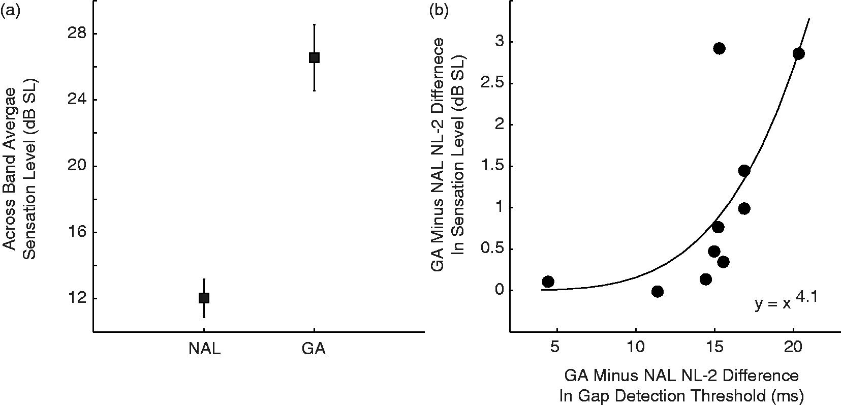

Discussion

The hearing aid prescriptions that are commonly used in clinics are based on rationales that focus on the long-term average spectrum of speech and therefore do not consider any distortions to the temporal envelope of speech that are introduced by hearing aid signal processing. Here, we demonstrated one way in which a prescription can be designed to minimize distortions to the shape of the temporal envelope. We used a GA to find the multiband compressor settings that maintained a strong correlation between the unmodified and hearing aid–modified temporal envelopes while also placing the modified envelope into the listener’s audiometric dynamic range. We did not set out to find the optimal setting for speech intelligibility or quality. Rather, the primary purpose of this work was to provide a proof of concept showing that a GA could be designed to create a hearing aid prescription that incorporates the preservation of the temporal shape.

The output of the GA provided an intuitive solution to temporal envelope shape preservation, which could be summarized by a simple set of rules. First, the compression threshold that resulted from the GA was a very low value that was near the minimum value of the speech envelope. By placing the compression threshold this low, any compression applied to the temporal envelope would scale low and high SPL values by equal amounts and thus preserve the shape of the original temporal envelope. Next, the GA-prescribed gain and compression ratio values boosted the level of the temporal envelope and compressed its range so that the bottom of the quiet speech envelope was near the audiometric threshold and the top of the 80 dB SPL speech envelope was near the UCL. This manipulation ensured that the entire speech temporal envelope was audible and comfortable. Instead, the compressor was nearly always using the attack time constant. As the attack time constant decreased, the smoothed temporal envelope (env, Equation [1]) that determined the amount of gain adjustment more closely matched the real-time speech envelope and therefore led to the least amount of temporal distortion.

The parameter setting rules that resulted from the GA optimization (excluding the time constants, where no comparison is possible) were similar to the rationale of a prescription that was designed to optimize audibility. In particular, there is a remarkable similarity between the fitting rule generated here and the one described in the DSL [i/o] prescription (Cornelisse et al., 1995). Much like the rule that resulted from the GA optimization, the rationale of DSL [i/o] was to compress the entire speech envelope and place it into the listener’s audiometric dynamic range. In contrast, there were substantial differences between the fitting rule generated here and the NAL-NL2 fit. The GA prescribed far more gain than did NAL-NL2, especially at the low frequencies (Figure 6). That less gain was prescribed by NAL-NL2 is likely due to the constraint on that formula ensuring that the loudness perceived by the hearing aid user does not exceed that perceived by an individual with normal hearing who was exposed to the same sound. The more extreme difference in low-frequency gain is likely due to the fact that NAL-NL2 is designed to optimize the SII. In this index, the low frequencies are given less weight because they are less important for speech intelligibility. Neither the DSL nor the NAL prescriptions assign time constants, and therefore, no comparison can be made in terms of these parameters. The work described here should not be used to determine which prescription is superior in terms of speech perception, quality, or comfort. Substantial behavioral testing would be necessary to make that claim.

The prescription determined here is an initial exploration, and further work is needed to develop this prescription into one that is clinically viable. We next consider a noncomprehensive list of factors that would need to be considered when further developing this prescription. First, the prescription as implemented here might be considered to be too loud for many patients. On average, the sensation level was 14 dB higher than NAL-NL2. Aversion to loud sounds is a primary concern of hearing aid users (Jenstad, Van Tasell, & Ewert, 2003), and the additional gain would likely exacerbate that problem. Anecdotally, no subject complained about the sound level. Second, our optimization only considered speech at input levels of 50 and 80 dB SPL. Input sounds that are higher than 80 dB SPL would exceed the patient’s UCL. This could be addressed by running the optimization while using a test signal that had a larger variation in overall level, as well as by incorporating limiter parameters into each gene. Finally, although the current GA prescribes considerable low-frequency gain, there are several practical considerations that suggest that such low-frequency gain could be problematic. For example, in some cases background noise is concentrated in the low frequencies, and therefore, boosting the low frequencies would effectively lower the signal-to-noise ratio. Further, it is well known that that low frequencies cause more masking of high frequencies than vice versa (e.g., Martin & Pickett, 1970). Therefore, boosting the low frequencies might mask the higher frequency portions of the signal that are known to be critical for speech perception. A future optimization would need to incorporate some penalty for boosting the low-frequency gain too much.

On the behavioral level, the GA led to better gap detection performance than did NAL-NL2 (Figure 7b), although the improvement might not have been attributable to preservation of temporal envelope shape. Acoustical analyses of the two prescriptions (Figure 8) revealed that, on the individual level, the extent to which the GA was louder was correlated with the extent to which the listener had better gap detection thresholds with the GA. This is consistent with observations that gap detection thresholds improve with presentation level (Fitzgibbons, 1983; Shailer & Moore, 1983). It is possible that this difference in gap detection performance was influenced by differences in presentation level, rather than the attempt to preserve the temporal envelope shape per se. In contrast, there were no differences in speech-in-noise performance between the two prescriptions. It is encouraging that the GA was at least as good as a conventional prescription in this regard.

The behavioral tests in this investigation were an initial exploration into the perceptual influence of this prescription. It is possible that a more subtle measure of temporal perception would reveal the perceptual consequences of these prescriptions. It is also possible that only a subset of hearing aid users would benefit from a prescription that preserves the temporal envelope shape. For example, it has previously been shown that only listeners with higher cognitive ability benefit from fast-acting compression (Gatehouse, Naylor, & Elberling, 2003). It might also be the case that such listeners are the ones who could benefit from a prescription that preserves temporal envelope shape.

Overall, this work demonstrates one method for considering distortions to the temporal envelope shape when designing a hearing aid prescription. Although the prescription described here is not ready to be deployed in the clinic, some aspects of this optimization could potentially be combined with existing hearing aid prescriptions—adding an additional theoretically based criterion to the rationale. Such combinations would enable these prescriptions to prescribe time constants and would ensure that the prescription provides minimal distortion to the temporal envelope shape.

Footnotes

Authors’ Note

Portions of this work were presented at the 2011 meeting of the American Auditory Society in Scottsdale, AZ, USA.

Declaration of Conflicting Interests

The author(s) declared no potential conflicts of interest with respect to the research, authorship, and/or publication of this article.

Funding

The author(s) disclosed receipt of the following financial support for the research, authorship, and/or publication of this article: This work was funded by the National Institutes of Health grant DC60014 and the Northwestern University Doctor of Audiology Program.

Acknowledgments

Holly Wiles, AuD, helped with human data collection.

References

ANSI. (2003). S3.22-2003, Specification of hearing aid characteristics. New York: Acoustical Society of America.

Baskent

Eiler

C. L.

Edwards

(2007) Using genetic algorithms with subjective input from human subjects: Implications for fitting hearing aids and cochlear implants. Ear and Hearing 28: 370–380.

Brennan, M. A., Gallun, F. J., Souza, P. E., & Stecker, C. (In Press). Temporal resolution with a prescriptive fitting formula. American Journal of Audiology.

Byrne

Dillon

Ching

Katsch

Keidser

(2001) NAL-NL1 procedure for fitting nonlinear hearing aids: Characteristics and comparisons with other procedures. Journal of the American Academy of Audiology 12: 37–51.

Cornelisse

L. E.

Seewald

R. C.

Jamieson

D. G.

(1995) The input/output formula: A theoretical approach to the fitting of personal amplification devices. Journal of the Acoustical Society of America 97: 1854–1864.

Cox

R. M.

Matesich

J. S.

Moore

J. N.

(1988) Distribution of short-term RMS levels in conversational speech. Journal of the Acoustical Society of America 84: 1100–1104.

Dillon

Storey

(1998) The National Acoustic Laboratories’ procedure for selecting the saturation sound pressure level of hearing aids: Theoretical derivation. Ear and Hearing 19: 255–266.

Drullman

Festen

J. M.

Plomp

(1994) Effect of temporal envelope smearing on speech reception. Journal of the Acoustical Society of America 95: 1053–1064.

Durant

E. A.

Wakefield

G. H.

(2002) Efficient model fitting using a genetic algorithm: Pole-zero approximations of HRTFs. IEEE Transactions on Speech and Audio Processing 10: 18–27.

10.

Durant

E. A.

Wakefield

G. H.

Van Tasell

D. J.

Rickert

M. E.

(2004) Efficient perceptual tuning of hearing aids with genetic algorithms. IEEE Transactions on Speech and Audio Processing 12: 144–155.

11.

Eddins

D. A.

Hall

J. W.

3rd Grose

J. H.

(1992) The detection of temporal gaps as a function of frequency region and absolute noise bandwidth. Journal of the Acoustical Society of America 91: 1069–1077.

12.

Fitzgibbons

P. J.

(1983) Temporal gap detection in noise as a function of frequency, bandwidth, and level. Journal of the Acoustical Society of America 74: 67–72.

13.

Gallun

Souza

(2008) Exploring the role of the modulation spectrum in phoneme recognition. Ear and Hearing 29: 800–813.

14.

Gatehouse

Naylor

Elberling

(2003) Benefits from hearing aids in relation to the interaction between the user and the environment. International Journal of Audiology 42(Suppl. 1): S77–S85.

15.

Glasberg

B. R.

Moore

B. C.

(1992) Effects of envelope fluctuations on gap detection. Hearing Research 64: 81–92.

16.

Grose

J. H.

Eddins

D. A.

Hall

J. W.

3rd (1989) Gap detection as a function of stimulus bandwidth with fixed high-frequency cutoff in normal-hearing and hearing-impaired listeners. Journal of the Acoustical Society of America 86: 1747–1755.

17.

Holube

Fredelake

Vlaming

Kollmeier

(2010) Development and analysis of an International Speech Test Signal (ISTS). International Journal of Audiology 49: 891–903.

18.

Jenstad

L. M.

Van Tasell

D. J.

Ewert

(2003) Hearing aid troubleshooting based on patients’ descriptions. Journal of the American Academy of Audiology 14: 347–360.

19.

Kates

J. M.

(2010) Understanding compression: Modeling the effects of dynamic-range compression in hearing aids. International Journal of Audiology 49: 395–409.

20.

Keidser

Dillon

Flax

Ching

Brewer

(2011) The NAL-NL2 prescription procedure. Audiology Research 1: 88–90.

21.

Killion

M. C.

Niquette

P. A.

Gudmundsen

G. I.

Revit

L. J.

Banerjee

(2004) Development of a quick speech-in-noise test for measuring signal-to-noise ratio loss in normal-hearing and hearing-impaired listeners. Journal of the Acoustical Society of America 116: 2395–2405.

22.

Levitt

(1971) Transformed up-down methods in psychoacoustics. Journal of the Acoustical Society of America 49: 467–477.

23.

Martin

E. S.

Pickett

J. M.

(1970) Sensorineural hearing loss and upward spread of masking. Journal of Speech and Hearing Research 13: 426–437.

24.

Moore

B. C.

(2008) The choice of compression speed in hearing AIDS: Theoretical and practical considerations and the role of individual differences. Trends in Amplification 12: 103–112.

25.

Moore

B. C.

Glasberg

B. R.

(2004) A revised model of loudness perception applied to cochlear hearing loss. Hearing Research 188: 70–88.

26.

Moore

B. C.

Glasberg

B. R.

Hess

R. F.

Birchall

J. P.

(1985) Effects of flanking noise bands on the rate of growth of loudness of tones in normal and recruiting ears. Journal of the Acoustical Society of America 77: 1505–1513.

27.

Naylor

Johannesson

R. B.

(2009) Long-term signal-to-noise ratio at the input and output of amplitude-compression systems. Journal of the American Academy of Audiology 20: 161–171.

28.

Payton

K. L.

Braida

L. D.

(1999) A method to determine the speech transmission index from speech waveforms. Journal of the Acoustical Society of America 106: 3637–3648.

29.

Rosen

(1992) Temporal information in speech: Acoustic, auditory and linguistic aspects. Philosophical Transactions of the Royal Society of London 336: 367–373.

30.

Scollie

Seewald

Cornelisse

Moodie

Bagatto

Laurnagaray

Pumford

(2005) The desired sensation level multistage input/output algorithm. Trends in Amplification 9: 159–197.

31.

Shailer

M. J.

Moore

B. C.

(1983) Gap detection as a function of frequency, bandwidth, and level. Journal of the Acoustical Society of America 74: 467–473.

32.

Souza

Gallun

(2010) Amplification and consonant modulation spectra. Ear and Hearing 31: 268–276.

33.

Souza

P. E.

(2002) Effects of compression on speech acoustics, intelligibility, and sound quality. Trends in Amplification 6: 131–165.

34.

Souza

P. E.

Jenstad

L. M.

Boike

K. T.

(2006) Measuring the acoustic effects of compression amplification on speech in noise. Journal of the Acoustical Society of America 119: 41–44.

35.

Stone

M. A.

Moore

B. C.

(1992) Syllabic compression: Effective compression ratios for signals modulated at different rates. British Journal of Audiology 26: 351–361.

36.

Stone

M. A.

Moore

B. C.

(2007) Quantifying the effects of fast-acting compression on the envelope of speech. Journal of the Acoustical Society of America 121: 1654–1664.

37.

Wakefield

G. H.

van den Honert

Parkinson

Lineaweaver

(2005) Genetic algorithms for adaptive psychophysical procedures: Recipient-directed design of speech-processor MAPs. Ear and Hearing 26: 57S–72S.

38.

Wiley

T. L.

Cruickshanks

K. J.

Nondahl

D. M.

Tweed

T. S.

Klein

B. E.

(1996) Tympanometric measures in older adults. Journal of the American Academy of Audiology 7: 260–268.

Initial Development of a Temporal-Envelope-Preserving Nonlinear Hearing Aid Prescription Using a Genetic Algorithm

Abstract

Keywords

Introduction

Experiment I: Algorithm Analysis

Method

Multiband compression

Filtering

Compression

Summation

Genetic Algorithm

Overview

Test audiograms

Test stimuli

Initialization

Evaluation of fitness

Determination of next generation

Stopping criterion

Results

Description

Acoustical comparison to NAL-NL2

Experiment II: Behavioral Testing

Method

Participants

Equipment

Prescriptions

Speech-in-noise testing

Gap detection

Results

Discussion

Footnotes

Authors’ Note

Declaration of Conflicting Interests

Funding

Acknowledgments

References