Sage Journals: Discover world-class research

Abstract

Users of bilateral cochlear implants (CIs) show above-chance performance in localizing the source of a sound in the azimuthal (horizontal) plane; although localization errors are far worse than for normal-hearing listeners, they are considerably better than for CI listeners with only one implant. In most previous studies, subjects had access to interaural level differences and to interaural time differences conveyed in the temporal envelope. Here, we present a binaural model that predicts the azimuthal direction of sound arrival from a two-channel input signal as it is received at the left and right CI processor. The model includes a replication of a clinical speech-coding strategy, a model of the electrode-nerve interface and binaural brainstem neurons, and three different prediction stages that are trained to map the neural response rate to an azimuthal angle. The model is trained and tested with various noise and speech stimuli created by means of virtual acoustics. Localization error patterns of the model match experimental data and are explicable largely in terms of the nonmonotonic relationship between interaural level difference and azimuthal angle.

Keywords

cochlear implant bilateral head-related transfer function interaural level difference lateral superior olive localization direction of arrival

Introduction

Normal-hearing (NH) subjects can localize the source of a sound with high acuity across a wide range of azimuthal (horizontal) locations. The highest precision that can be achieved for azimuthal differences in the frontal field—the minimum audible angle—is approximately 1° (e.g., Mills, 1958). The explanation for this precision has been attributed to exquisite sensitivity to interaural time differences (ITDs) conveyed in the temporal fine structure of low-frequency sounds, particularly in the frequency range of 500 to 800 Hz (Wightman & Kistler, 1992). Cochlear implant (CI) listeners are generally unable to exploit this cue, even with identical CI processors in both ears. One of the reasons is that the ITD is often not preserved in the electrical pulse timing. Another reason is that most CI listeners are insensitive to ITDs if the electrical pulse trains that convey ITDs are presented at a rate greater than 500 pulses per second (pps; e.g., Majdak, Laback, & Baumgartner, 2006). CI listeners instead rely on other localization cues that are generally available to both NH and bilaterally implanted listeners, such as ITDs conveyed in the temporal envelope of modulated sounds (envelope ITDs) and interaural level differences (ILDs). Spectral cues generated by the interaction of the sound with the head and outer ears also contribute to some degree to localization performance in both the horizontal and vertical planes and are available even in monaural listening. The extent to which CI users can exploit these cues, however, is further limited by the microphone position, the CI processing, and the spread of excitation. Together these aspects result in the very limited localization performance of unilateral CI listeners (Kerber & Seeber, 2012).

Localization performance is typically assessed with broadband noise (e.g., Kerber & Seeber, 2012) or speech stimuli (e.g., Potts, Skinner, Litovsky, Strube, & Kuk, 2009) presented via loudspeakers in free-field conditions to provide a wide range of localization cues. The localization performance of different listener groups can then be directly inferred from the availability and absence of the localization cues. Compared with unilateral CIs, the use of bilateral CIs greatly improves the accuracy with which sounds can be localized in the azimuthal plane (e.g., Litovsky, Parkinson, & Arcaroli, 2009; Nopp, Schleich, & D’haese, 2004), which can be attributed to bilateral CI users exploiting the ILD, and potentially the envelope ITD, in their judgments (Laback, Pok, Baumgartner, Deutsch, & Schmid, 2004; Seeber & Fastl, 2008). Nevertheless, most studies reveal a substantial gap in localization performance between NH listeners and users of bilateral CIs (Grantham, Ashmead, Ricketts, Labadie, & Haynes, 2007; Litovsky et al., 2012), likely resulting from of the lack of fine-structure ITD information, as well as the independent operation of left and right CI devices, left and right differences in the processor settings, and the electrode-nerve interfaces. Kerber and Seeber (2012) tested the localization ability of NH listeners, bilateral CI users, and unilateral CI users in the same task. Their results revealed a median root mean square (RMS) localization error of about 5° for NH listeners, 30° for bilateral CI listeners, and 47° for the two best performing unilateral CI listeners, whilst two other unilateral listeners were unable even to discriminate between left and right. Távora-Vieira, De Ceulaer, Govaerts, and Rajan (2015) further showed that CI subjects suffering from unilateral deafness showed significant improvements in localization abilities when the CI was switched on (mean RMS error = 22.8°) compared with when it was not (mean RMS error = 48.9°), despite the very different sound stimulation provided to each ear.

To gain a deeper insight into the origin of the localization errors made by bilateral CI subjects, Jones, Kan, and Litovsky (2014) compared their performance with that of NH listeners listening through a vocoder simulation of virtual acoustic sounds. They found comparable performance of about 30° RMS error and a very similar pattern of systematic errors. The comparison of CI data with NH data using vocoder simulations has proven beneficial in the past because the simulations enable testing of two almost identical ears with identical preprocessing and also show a low intersubject variability (e.g., Goupell & Litovsky, 2014). Therefore, the comparable performances between vocoded NH and CI subjects reported by Jones et al. suggest that the absence of fine-structure ITD is the most limiting performance factor with differences between left and right CI playing a less critical role.

Of the remaining two interaural cues available to typical bilateral CI users, namely envelope ITDs and ILDs, the latter is the more salient and dominant cue (Laback et al., 2004; Seeber & Fastl, 2008). Using their clinical speech processors, subjects could discriminate acoustic ILDs of approximately 2 dB, only about twice as high as NH listeners (Laback et al., 2004).

Despite ILDs being the most important cue for sound source localization with bilateral CIs, little information exists as to how the azimuthal direction of sound arrival translates into different electrode activations, different auditory nerve (AN) response rates, and, ultimately, in listeners being able to perceive the direction of sound arrival. Computer models complemented by experimental data are expected to reveal this, by dissecting the specific contribution of each stage of the long processing chain. For example, some monaural models combine a speech-coding strategy with a model of the electrode-nerve interface (e.g., Imennov & Rubinstein, 2009; Stadler & Leijon, 2009). Such models are useful in clarifying whether specific differences between electric and acoustic hearing are caused by the speech-coding strategy or rather by the electrode-nerve interface. To understand spatial hearing with CIs, even more processing stages are required, namely the filtering of the sound by the head and torso, typically referred to as the direction-dependent head-related transfer function (HRTF) as a front end and the binaural interaction as additional back end.

To date, such direction-estimating models exist only for NH listeners (e.g., Dietz, Ewert, & Hohmann, 2011; Faller & Merimaa, 2004). They have found various applications in wave field synthesis (e.g., Wierstorf, Raake, & Spors, 2013), computational auditory scene analysis (Spille, Meyer, Dietz, & Hohmann, 2013b; Woodruff & Wang, 2013), and automatic speech recognition (e.g., Spille, Dietz, Hohmann, & Meyer, 2013a). Direction-estimating models for bilateral CI listeners could further be applied to CI algorithm development or individualized performance prediction. However, existing binaural models of CI listening (e.g., Chung, Delgutte, & Colburn, 2014; Colburn, Chung, Zhou, & Brughera, 2009; Nicoletti, Wirtz, & Hemmert, 2013) have mostly been concerned with the response of binaural neurons in the brainstem to electrical stimulation. So far, no published CI model combines all necessary processing stages required to estimate the direction of sound arrival based on simulated neural responses.

Here, we present a processing chain for modeling the spatial hearing of bilateral CI listeners by combining several existing models. The processing chain includes (a) the sound interacting with the HRTF, (b) the CI speech processor, (c) the electrode-nerve interface, (d) a model of the AN responses, (e) a neural stage of binaural processing, and (f) three models of a mapping stage, which estimate an azimuthal direction of the sound source based on the neural left and right input. Investigating the input–output characteristics of the key stages and the nonlinear interaction of some stages will allow for a detailed investigation of the final prediction and of any systematic error. The model-based estimates will also be compared against published data and be used to test hypotheses made in the previously described studies. In particular, the dominance of the ILD and the detrimental effect of the level-dependent compression will be investigated.

Methods

The model was implemented in MATLAB. The code is publicly available.¹

After introducing the stimuli used, the following subsections will follow the processing chain of the stimuli by the model stages as illustrated in Figure 1.

Figure 1.

Flow chart of the implemented processing chain. Each stage is described in detail in the Methods section. The localization models operate either on the AN output or on the output of the binaural interaction stage (see last part of the Methods section for details). The output of the binaural interaction stage still has two channels, representing left and right hemisphere brainstem neurons.

Stimuli and HRTF Filtering

Four different stimuli were used to test the model:

Stationary speech-shaped noise (SSN) generated from 10 male and 10 female adult German speakers, uttering sentences of the Oldenburg Sentence Test (OLSA) by the procedure described in Wagener, Kühnel, and Kollmeier (1999): OLSA noise OL-noise (SSN),

Pink noise (PN), that is, stationary noise with a 1/f power spectrum,

White Gaussian noise (WN), and

A male frozen speech segment (Sp) taken from the OLSA consisting of the phone [vaI̯] from the German word weiß.

Dichotic, free-field stimuli were produced from these four stimuli using a previously generated database of head-related impulse responses (Kayser et al., 2009). The head-related impulse responses were taken from the frontal out of the three behind-the-ear microphones mounted on an artificial human head and torso at a virtual source distance of 3 m. The free-field stimuli were then generated at 5° intervals for the azimuthal angles between 0° and 90°, generating 19 virtual sources for each stimulus.

All experimental stimuli were 200 ms in duration and adjusted to have 10-ms rise and fall times. Model experiments were performed at three different stimulus levels of 45, 55, and 65 dB sound pressure level (SPL) for the frontal source direction. When the signal was presented from a nonfrontal direction, the same calibration was used, and the level would deviate from the frontal level.

In addition to these four main stimuli, two more natural stimuli were used for additional testing. One was 10 s of continuous male and female speech, obtained from the OLSA, to examine predictive ability in the case of dynamic level fluctuations. The second was SSN combined with a 360° white noise interferer at 5 dB signal-to-interferer ratio to examine the effects of interfering sound on the predictive ability of the model.

CI Processing

The transformation from sound to electrodogram was performed using the advanced combination encoder (ACE) strategy implemented in the Cochlear Nucleus 24 implant (Laneau, 2005). The acoustic broadband signal was sampled at 16 kHz and filtered into 22 frequency bands using a 128-point FFT. The frequency bands had center frequencies linearly spaced below 1000 Hz and logarithmically spaced above 1000 Hz. As part of the ACE processing strategy, an n-of-m strategy was implemented by selecting the 8 most energetic of the 22 channels in each 8-ms time frame. Out of the eight selected bands, the most basal band was stimulated first during each time frame, followed sequentially by the next one. Frequency-independent compression was then performed on each channel by applying a loudness growth function with a steepness controlled by the parameter α_c = 415.96 (see Swanson, 2008 for further details). Threshold levels of T_SPL = 25 dB SPL and maximum levels M_SPL = 65 dB SPL were set, and the resulting levels were then mapped to the CI electrode threshold and saturation levels that were specified in clinical units (CL) of T = 100 CL and M = 200 CL, respectively. These values were then mapped onto output current values, $I in μ A$ , by using the device-specific mapping function, $I = 10 . 175^{CL - 100}$ . Finally, biphasic pulses with 25-µs phase duration (cathodic first) and an 8-µs interphase gap were generated in a monopolar stimulation mode and sent to the virtual CI at a rate of 900 pps.

Electrode-Nerve Interface

The spread of current within the cochlea and the response of the population of AN fibers was modeled as in Fredelake and Hohmann (2012). The model assumed an unwound cochlea with a length of 35 mm. The 22 electrodes were equally distributed between 8.125 and 23.875 mm (measured from the apex) at a spacing of 0.75 mm, simulating a Cochlear Nucleus 24 electrode array. The electrode locations inside this virtual cochlea corresponded to acoustic frequencies between 363 and 4332 Hz according to the frequency-to-place function of Greenwood (1990). The spread of current in the cochlea was modeled by a double-sided, one-dimensional, exponentially decaying spatial-spread function controlled with the parameter λ = 9 mm. Along the virtual cochlea, 500 AN fibers were equally distributed. To simulate individual AN fiber stimulation to electric pulses, the electric pulse trains were processed by a deterministic leaky integrate-and-fire model (Gerstner & Kistler, 2002) extended with a zero-mean Gaussian noise source, to simulate stochastic behavior of the AN fibers. The model processed electric pulse trains with a stimulus-level-dependent current amplitude across electrodes as input. The model output was a vector of AN spike times over the duration of the acoustic stimulus for each AN fiber in the population.

AN Frequency Bands

Models of binaural processing assume convergent input from a certain number of AN fibers. The model described in the binaural interaction stage used 20 AN inputs from either side (Wang & Colburn, 2012) so that sample groups of 20 fibers along the model cochlea were combined for further analysis of the AN responses. Instead of presenting all 25 possible AN groups from the 500 fibers, only five sample groups were selected, centered at 10, 13, 16, 19, and 22 mm from the apex, corresponding to 5 segments, each covering 2 electrodes in the range of electrodes 3 to 20. The five mean center frequencies of the five electrode pairs were 563, 1063, 1813, 3188, and 5500 Hz. To compute the corresponding acoustic free-field ILDs, left and right audio channels were filtered using equivalent rectangular bandwidth-wide fourth-order gammatone filters (Hohmann, 2002) with the same five center frequencies mentioned earlier. The RMS power was computed in each frequency band and the difference between the right and left channels produced the final frequency-dependent ILD.

Binaural Interaction Stage

A Hodgkin–Huxley-type model was used to model binaural interaction at the level of the brainstem (Wang & Colburn, 2012). The single-compartment model contained a sodium channel, a high-threshold potassium channel, and a passive leak channel. All channel and membrane parameters were chosen in the original study to be within the plausible range for the lateral superior olive (LSO; see Wang & Colburn, 2012 for more details). Each binaural model neuron received 20 excitatory AN inputs from the ipsilateral side and 20 inhibitory inputs from the contralateral side that corresponded to the AN frequency bands described earlier. When using the electric stimulation front end, it was found that the output responses of the original model parameters did not generate ILD- or ITD-dependent output over the tested range. Therefore, as in Wang, Devore, Delgutte, and Colburn (2014), the excitatory and inhibitory conductances of the LSO model were reduced compared with the Wang and Colburn (2012) conductances. The final chosen values for the current study were 1.2 and 1.0 nS, respectively, which were still within the physiologically plausible range.

Localization Models

The stages presented so far modeled the neural response rates at the AN and LSO stages in the five AN frequency bands. The neural response rates are expected to change depending on the source location. In this subsection, three different localization models are proposed to map the response rate differences to a predicted source location. The methods, namely linear rate-level localization, linear response difference localization, and maximum-likelihood localization, were implemented on the interaural AN response differences or on the respective LSO response differences. Each model differs from the others in the choice of input–output relations that were used to train the model.

Linear rate-level localization model

This model operates only on AN responses, not on LSO responses. Compared with the other two model types that will be introduced, this model allows for a more functional understanding of the input–output relations of each processing stage shown in Figure 1, thus enabling the user to pinpoint the origin of model predictions to the influence of acoustic ILDs, the influence of speech coding, or influences at the electrode-nerve interface. The model assumes a priori claims that (1) ILD can be linearly mapped to azimuthal direction of sound arrival, (2) monaural AN response rate can be linearly mapped to stimulus level, and (3) CI subjects’ percept of azimuthal localization can be linearly mapped to the interaural AN response rate difference $(R right - R left) n$ in each frequency band, where n denotes the frequency band index. All three claims are fairly crude assumptions that are typically not fulfilled. For example, the ILD is not even monotonic as a function of azimuth (e.g., Macaulay, Hartmann, & Rakerd, 2010). Nevertheless, it will be demonstrated that Claims (1) and (3) are very accurate at central angles between −45° and +45°.

Thirty instances of 200-ms SSN were HRTF filtered and the virtual source at 0° was presented monaurally. Monaural rate-level curves were constructed from the mean AN response rates within each of the AN frequency bands, and, based on Claim (2), a linear regression was performed on this data between the SPL of 35 and 70 dB. The slopes b_n (Figure 2, bottom left panel) of these linear approximations represent the response rate change per dB for a given frequency band n.

Figure 2.

Schematics of the localization models via linear fitting. (Left): two-stage rate-level localization model. The first stage maps azimuthal angle to ILD, and the second stage maps level to spike rate. These two mappings produce a final mapping of AN response rate difference to azimuthal angle. (Right): response rate difference localization model. This model is used on the interaural response difference for either the AN or the LSO output.

Figure 3.

(Top): Ipsilateral (dashed lines) and contralateral levels (solid lines) relative to 0° plotted as a function of azimuthal angle for the five AN frequency bands. (Bottom): Interaural level difference (ILD) as a function of azimuthal angle for the five AN frequency bands.

For training the model to the frequency-dependent mapping of ILD to azimuth, the SSNs were presented (in virtual acoustic space) from each of the azimuthal angles. A further linear regression (based on Claims 1 and 3) generated a slope m_n that linearly mapped ILD to an azimuthal angle for each of the AN frequency bands (Figure 2, top left panel). As the model is inherently left–right symmetric, the analysis can be limited to sounds originating from the right hemisphere without loss of generality. The only consequence of the right hemisphere restriction together with the symmetry assumption is that the linear regression has to be forced to be point-symmetric as well. This is achieved by setting the y axis intercept to zero and fitting only the slope.

In each frequency band n, the predicted direction of sound arrival $α n$ was then determined by the interaural AN response rate differences divided by the products of the rate-level slope $b n$ and the ILD per degree azimuth slope m_n (see Figure 2):

α n = \frac{(R right - R left) n}{b n \cdot m n}

This functional relationship can be isolated again into the two stages used for training: Dividing the AN-rate difference by the rate-level slope

b n

determines the predicted ILD and dividing this quotient by m_n determines the predicted azimuth.

Two different model calibrations were generated by altering the azimuthal angle range over which the linear regression was computed: Slope m45 attempted to optimize performance in the central linear segment of the ILD to azimuthal angle function (Figure 2). The shallower slope m90 attempted to minimize the RMS error over the entire range.

To produce a final prediction from the five AN frequency bands, a rate-weighted average was then derived:

α weighted average = \frac{\sum_{n} α n (R right + R left) n}{\sum_{n} (R right + R left) n}

Linear response difference localization model

This model assumes the a priori claim that interaural response rate differences can be linearly mapped to CI subjects’ azimuthal localization percept. This model operates on the LSO responses; however, for a more direct comparison with the rate-level model, a second version of this model was used on the AN responses. In contrast to the linear rate-level model described earlier, the internal processing stages here are considered as a black box so that the model could be trained directly with the interaural response rate difference over azimuth functions for each frequency band. Because both the rate-level and the ILD-over-azimuth function are nonlinear, the single-stage linear calibration of AN-rate difference over azimuth is not necessarily the same as the combination of the two linear mappings performed in the previously described two-stage model. Presumably, this one-stage mapping is more accurate and at least more direct; however, the disadvantage over the two-stage rate-level calibration is its black-box approach. While good for applications, it does not allow the scientist to analyze the contribution of each processing stage. Training was performed with 30 instances of 55 dB SSN-noise convolved with the HRTF at each of the 19 sound source directions. Response rate differences were taken from 20 contralateral and 20 ipsilateral AN fibers. The output of these 40 fibers was then further processed by a binaural interaction stage that produced a contralateral–ipsilateral difference of one left and one right hemisphere LSO neuron per AN frequency band. Linear regressions on the spike rate data produced slopes that map azimuthal angle to spike rate differences. As in the previous AN-based localization model, the linear mapping coefficient

α n

was then derived by dividing the response rate differences between the two model LSO neurons by the slopes of the linear regression (Figure 2 and Table 1). Finally, a weighted average across frequency bands was computed using the same method described earlier.

Table 1.

Slopes of Linear Regression Performed for Each Stage of Localization Models Obtained With 55 dB Speech-Shaped Noise.

Localization model	AN frequency bands
Localization model	563 Hz	1063 Hz	1813 Hz	3188 Hz	5500 Hz
Rate-level
AN (b_n in R/dB)	16.56	14.75	15.06	13.23	13.30
-m45 (m_n in dB/°)	0.10	0.19	0.17	0.30	0.41
-m90 (m_n in dB/°)	0.06	0.10	0.12	0.20	0.30
Response rate difference
AN m45 ( $m n Δ R$ /°)	1.36	3.17	3.15	3.86	4.69
AN m90 ( $m n Δ R$ /°)	0.85	1.54	1.85	2.86	3.14
LSO m45 ( $m n Δ R$ /°)	1.67	2.53	2.26	2.97	3.00
LSO m90 ( $m n Δ R$ /°)	1.00	1.24	1.42	2.18	2.07

Note. AN = auditory nerve; LSO = lateral superior olive.

Maximum-likelihood estimation

This model assumes that localization can be modeled as maximizing the likelihood of a set of frequency channels over all possible azimuthal angle percepts, similar to the approach of Day and Delgutte (2013). A prediction was produced by performing a maximum-likelihood estimation (MLE) over all angles. This method exploits the azimuth-specific ILD patterns across frequency channels that are also mirrored by LSO neurons (Tollin & Yin, 2002). The MLE method includes, but is not limited to, a possible explicit place coding of ILD that will be detailed in the HRTF Results and Discussion section: Depending on which specific frequency channel is closest to its maximum ILD, the prediction model derives the corresponding azimuth. Hypothetically, this place-coding strategy is suitable at lateral angles, whereas, for more central angles, the probabilistic calibration can effectively operate in terms of a rate code, similar to the other calibrations. The model was trained with interaural AN response rate differences. As this prediction stage is more suited to training with naturally fluctuating signals, rather than long-term averages, 10 s of 55 dB SPL continuous male and female speech originating from each of the 19 possible directions was used as training material. Sample means, and corresponding standard deviations, were computed on response difference data collected in 200-ms windows for each of the 5 frequency bands resulting in 50 × 19 training events. A multivariate Gaussian distribution of response rate differences was then assumed at each angle. In contrast to the other models, this model is restricted to the right hemisphere by the training. However, this limitation can easily be overcome.

In the testing phase, only the five rate differences were supplied to the multivariate probability density function and the angle with the maximum likelihood was determined. This calibration method offers the advantage over the other two calibrations in that it can potentially cope with the nonmonotonic ILD because the azimuth dependence of the ILD is frequency specific, and each angle has its unique combination of ILDs. Because the training material and nature of the calibration was fundamentally different than that of the other linear methods, the maximum-likelihood results were not included in the statistical analysis of the other calibrations.

Results and Discussion

Influence of the HRTF

The upper torso and the head have a considerable spectral filtering effect that depends critically on the direction of sound arrival, especially for wavelengths shorter than head diameter (f > 1.5 kHz) (Figure 3). This is manifest as the HRTF (see, e.g., Kayser et al., 2009). However, even for sounds arriving from straight ahead, HRTF filtering results in a strong spectral coloration (Figure 4).

Whilst the difference in HRTFs between the ears for lateral sources is well known, and forms the basis of numerous investigations of spatial hearing (e.g., Strutt, 1907), the spectral coloration is typically not considered in studies that are not explicitly concerned with directional hearing. The importance of HRTFs, even for investigations into dimensions of sound processing other than localization, however, is apparent in the transfer function of the HRTF filtering to white noise at 0° azimuth and elevation (Figure 4), where a significant amplification of ∼5 dB SPL is evident in the 2 to 4 kHz range. A collateral benefit of this filtering is an enhancement of the higher frequency formants (1.7, 3.4, 4.3 kHz) that are captured in the corresponding AN frequency bands. The HRTF-filtered white noise also shows a high-pass characteristic resulting in approximate 10 dB attenuation at 200 Hz.

Figure 4.

Smoothed spectra of the four stimuli at 0° with and without HRTF filtering. Top left: speech-shaped noise (SSN). Top right: A 200-ms male speech token (Sp). Bottom left: 1/f pink noise (PN). Bottom right: White Gaussian noise (WN). The colored rectangles represent the AN frequency bands used in the localization models. The respective color corresponds to the color code introduced in Figure 3.

In contrast to the lack of HRTF consideration in monaural studies, many investigations have analyzed the azimuth dependence of the HRTF (e.g., Duda & Martens, 1998). In the current study, compared with a reference at 0° azimuth, ipsilateral signal levels increased slightly up to azimuthal angles of approximately 45° and flattened beyond that (Figure 3, top). This effect was relatively independent of sound frequency, with the exception of the 3188-Hz band, which showed destructive interference effects (due to the reflections from the shoulder) for angles beyond 45°. Conversely, contralateral levels were strongly dependent on azimuth over the entire range of angles. This effect was highly frequency dependent, with larger negative slopes corresponding to higher frequencies. This frequency dependence is well established and indeed was highlighted in early descriptions of the duplex theory of sound localization (Strutt, 1907). Low-frequency sounds have a longer wavelength than the diameter of the head and, as a result, are less subject to attenuation at locations contralateral to the source. This results in a frequency-dependent mapping of interaural difference to azimuth, expressed by the slopes m_n (see Table 1).

Contralateral levels dropped with increasing azimuthal angle up to a frequency-dependent minimum, after which they began to rise again. This increase toward 90° has been analytically described with a spherical head model (e.g., Duda & Martens, 1998): Close to −90°, the pathways around the head are similarly long and the waves interfere constructively at the contralateral ear. At midfrequencies (e.g., 1 kHz), this effect is already apparent at −60°, but at higher frequencies with shorter wavelength, the constructive interference began to appear only at more lateral angles (see Figure 3).

The free-field dependence of ILD on azimuthal angle was dominated by the contralateral effects (Figure 3, bottom). Due to the nonmonotonic behavior, it is not possible to generate a linear mapping of ILD to azimuth without including systematic errors. It is possible that the brain potentially learns this pattern of ambiguity and employs some form of explicit code to map this region, such that the dominant frequency of the neuron with the peak ILD determines the azimuth. The proposed MLE localization model can potentially account for this possibility, whereas the other localization models are limited by their linear approximations.

Influence of the CI Processing

One aspect that illustrates the interaction of HRTF influences and CI processing is the spectral filtering of the HRTF, which was shown to have relevance beyond azimuthal localization. These spectral filtering properties of the head, torso, and outer ear are typically only investigated when studying localization in the sagittal plane (e.g., Majdak, Goupell, & Laback, 2011). Their particular relevance for electric hearing can be seen in Figure 5, when comparing the monaural AN model output with and without HRTF filtering from 0° azimuth. For instance, the 1/f (pink) noise had the same energy in each octave band and elicited similar activations in all five frequency channels without HRTF preprocessing but possessed a very frequency-dependent activation after 0° HRTF filtering (Figure 5, column 3). Interestingly, this was precisely opposite to the case when SSN is assessed; here, the HRTF-filtered signal yielded the most homogeneous electrode activation (Figure 5, column 1). This illustrates just how well CI processing is tailored to match free-field HRTF filtering and the average speech spectrum. It is, therefore, important to include HRTF filtering for the purpose of modeling realistic response patterns for broadband stimuli even in monaural studies. CI subjects are also exposed to a similar HRTF filtering when they listen using their behind-the-ear microphones.

Figure 5.

(Top row) Cumulative charge output for each of the AN frequency bands of the four HRTF-filtered stimuli at 0°. The charge is summed over the 2 electrodes in each bin for the 200-ms duration of the stimuli. (Middle row) Mean AN frequency band rate-level curves for the same free-field stimuli. (Bottom row) Mean AN frequency band rate-level curves for the nonfree-field stimuli.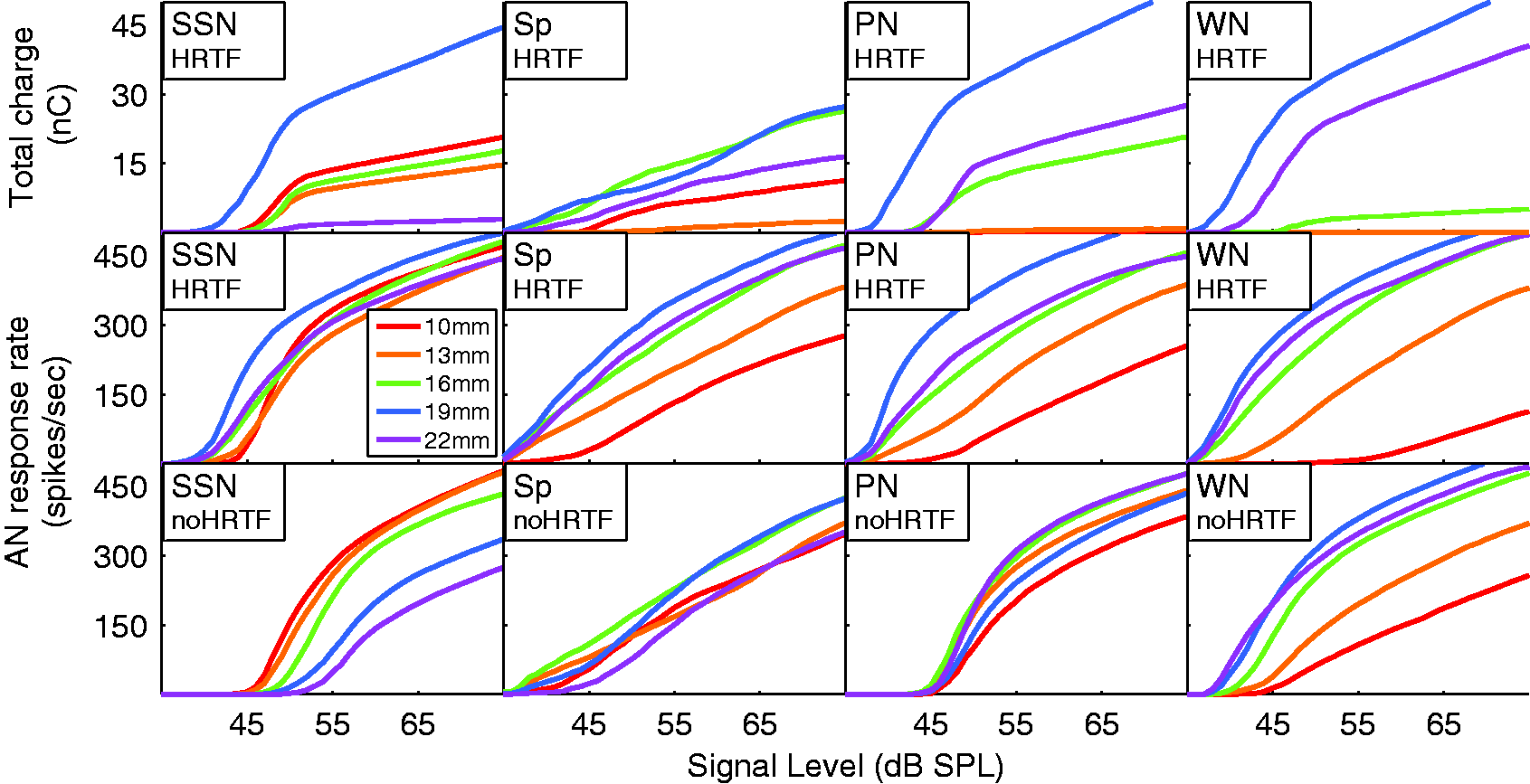

To map the large dynamic range of input signals—primarily of speech—to the low dynamic range of CI listeners, a relatively strong compression to the input signal is applied, which generates a nonlinear relationship between input level in dB and output current (Figure 5). This nonlinearity leads to a level-dependent transformation from ILD to interaural current differences (ICD). In the model, this ultimately resulted in level-dependent localization. At low input levels, where the compression was weak, a given ILD resulted in a larger ICD than at high input levels. This model prediction calls for a subjective evaluation of whether CI subjects show level-dependent localization. Level-dependent lateralization has been demonstrated with NH subjects with conflicting ITD information (Dietz, Ewert, & Hohmann, 2009) and bimodal listeners with nonmatched loudness growth (Francart & MacDermott, 2012). However, we are aware of only one bilateral CI subject whose localization abilities were tested at different levels (60 and 70 dB SPL; van Hoesel, Ramsden, & O’Driscoll, 2002). In line with our model prediction, van Hoesel et al. (2002) argues that level compression likely also has a compressive effect on the perceived angle at higher sound levels (i.e., it causes a central localization bias). Their single subject, in contrast, has a lateral localization bias at 70 dB SPL. This is further backed by data from Grantham, Ashmead, Ricketts, Haynes, and Labadie (2008; their Figure 3) that reveals lower ILD thresholds for bilateral CI subjects when compression is switched off.

Finally, performance is reduced by the independently operating n-of-m strategies in either processor (i.e., either ear). Due to the frequency dependence of ILDs, the contralateral ear had a bias to lower frequencies, resulting in the n-of-m strategy selecting more apical electrodes that were potentially not selected on the ipsilateral side. In some cases, this result led to a stronger stimulation on the contralateral electrodes and, ultimately, a contralateral localization cue in the apical channels (see PN: 65 dB, Figure 7, top right). A similar effect has previously been described for independently operating gain control in each ear (Dorman et al., 2014).

The HRTF-filtered SSN produced the most uniform stimulation pattern across all sound levels, and the dynamic range from approximately 40 to 70 dB SPL was centered around 55 dB (Figure 5, middle left). Because of these properties, 55 dB SSN was chosen to calibrate the localization models. In the case of speech being used as a test stimulus, the instantaneous level fluctuations resulted in a more linear mean stimulus level across the stimulation current curve (Figure 5, second column).

Influence of Spread of Excitation

The spread of current within the cochlea is the major limiting factor of spectral resolution in electric hearing (Bingabr, Espinoza-Varas, & Loizou, 2008). With a 9 mm exponential current decay, and an AN frequency band spacing of just 1.4 mm, a considerable cross talk can be expected. This was visible in the AN-rate-versus-azimuth functions (Figure 6), where differences between neighboring channels were reduced compared with the acoustic ILDs (Figure 3). However, in the tested conditions, with one directional source, even this large spread of excitation did not systematically influence localization ability. Similarly, even an interaural electrode mismatch has been shown not to harm ILD sensitivity very much (Kan, Stoelb, Litovsky, & Goupell, 2013). Further, in a two-source condition, with both sources having different frequency content, spread of excitation would be expected to impact localization more than we demonstrate here. Finally, the spread of excitation resulted in a less reliable relation of response rate difference for a given azimuth. For instance, the peak of the AN-rate difference over azimuth (Figure 6) was at 70° for both the 19- and the 22-mm channel, whereas the corresponding acoustic ILD had peaks at 70° and 80°, respectively. The spread from the more energetic electrodes around the 19-mm band to the 22-mm band caused the 22-mm rate difference to be dominated by off-frequency ILDs.

Figure 6.

AN response rate differences for speech-shaped noise at three different levels. (Top) Right (dashed lines) and left AN response rates relative to a 0° reference are plotted as a function of azimuthal angle for the five AN frequency bands. (Bottom) Interaural AN response rate difference as a function of azimuthal angle for the AN frequency bands. The respective color corresponds to the color code as in Figures 3 and 4. The level dependence is due to flooring effects at the contralateral left side (no responses) at 45 dB and strong compression effects especially at the right side at 65 dB.

Figure 7.

(Top) Interaural AN response rate difference as a function of azimuthal angle for the 5 AN frequency bands to speech-shaped noise (left) and pink noise (right) at 65 dB. (Bottom) Interaural LSO response rate difference as a function of azimuthal angle for the five AN frequency bands to speech-shaped noise (left) and pink noise (right). The respective color corresponds to the same frequency bins as in previous figures.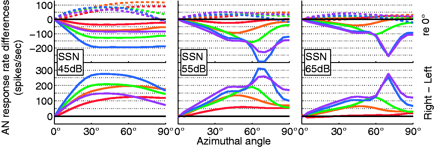

Influence of the Binaural Model

Whilst the difference between interaural AN responses purely resembled the ILD cue, the modeled binaural neurons were also sensitive to the ITD. In the case of the ACE strategy assessed here, the only available ITD cue was the envelope ITD. In clinical processors, ILD cues dominate envelope ITD cues for both speech and noise input (Laback et al., 2004). This is in line with the model outcome, that is, that the LSO output as a function of azimuth (Figure 7) had a similar shape to that of the acoustic ILDs (Figure 3). When comparing LSO model data with AN model data (Figure 7), the small but positive influence of envelope ITD can be seen in the 22-mm channel where the decline toward 90° was smaller in the LSO than in the AN response. The LSO stage of the model is expected to be suitable for testing potential localization benefits of new coding strategies that preserve ITD in the pulse timing.

NH listeners can also exploit temporal fine-structure ITD information in the 1-kHz regime, presumably through their faster medial superior olive (MSO) pathway (Remme et al., 2014). In processing binaural information, CI listeners appear to be limited to the slower LSO pathway, consistent with their upper-frequency limen being roughly 200 to 400 Hz or pps, even if ITDs are preserved in the pulse pattern (van Hoesel & Clark, 1997; van Hoesel & Tyler, 2003). A possible reason for CIs not activating the MSO pathway is that the highly synchronized neural stimulation pattern from the electric pulses is not optimal for the synapse and membrane parameters of the MSO (Chung et al., 2014). This single effective pathway of the LSO was represented by our model and contrasts with the complex dual (MSO, LSO) pathway models of the acoustically stimulated binaural system (e.g., Dietz et al., 2009; Hancock & Delgutte, 2004; Takanen, Santala, & Pulkki, 2014).

Results of the Localization Models

In contrast to the previous stages, less is known about how central pathway stages extract a localization percept from the ensemble of binaural brainstem neurons. Therefore, three different localization models were tested here. The first strategy was a two-stage linear mapping of the monaural AN response rates into level and from ILD to azimuth. This strategy is less likely to resemble the physiologic processes or the learning and estimating strategies of a human subject (Figure 8(a)). The second localization model of a one-stage linear mapping from interaural rate differences of LSO or AN responses to azimuth is more plausible, at least as a possible learning strategy of a listeners brain (Figures 8(b) and 9).

Figure 8.

Model predictions and RMS error for the rate-level and response difference localization models. Frequency band predictions are shown for the SSN stimulus at 55 dB. Weighted average predictions are also shown (black) for all levels tested with the model. (Left) Predictions using the AN-rate-level m45 localization model. (Right) Predictions using the AN response difference m45 localization model.

Figure 9.

Model predictions and RMS error for the AN (Left) and LSO (Right) response difference localization models for the m90 slope calibration. AN frequency band predictions are shown for the SSN stimulus at 55 dB. Weighted average predictions are also shown (black) for all levels tested with the model.

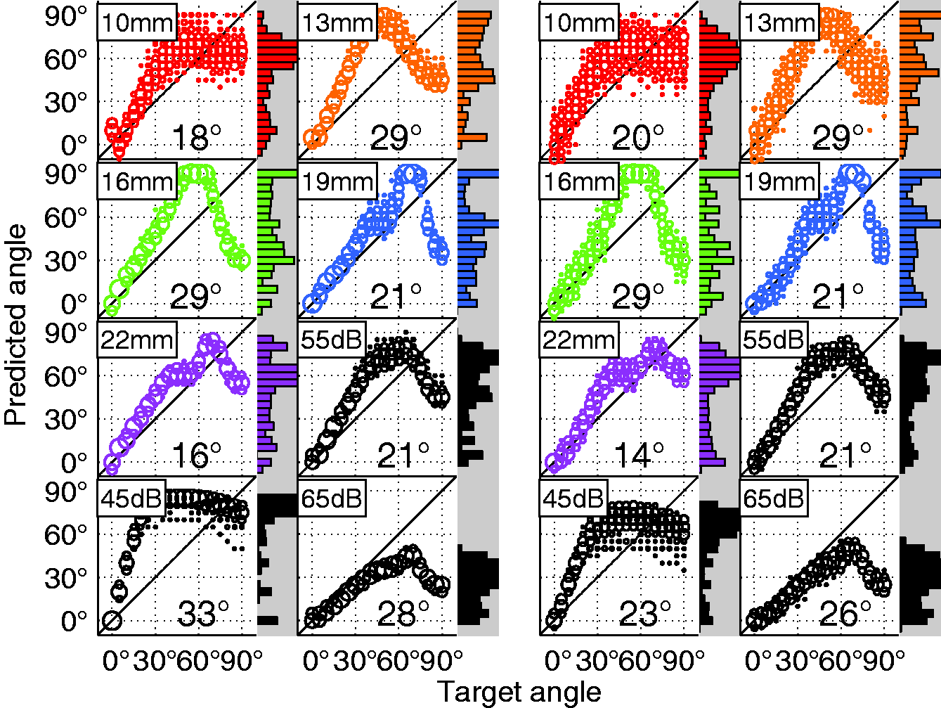
The calibration of the linear mapping was somewhat arbitrary; however, it could resemble an individual mapping strategy. For instance, Jones et al. (2014) reported very individualized localization estimation patterns that can be attributed to such mappings. Two possible mapping strategies were tested here: (a) minimizing the error in the frontal segment between −45° and +45° and (b) minimizing the error in the range between −90° and +90°. Both strategies were successful in reaching their specific goal (Figures 8(b) and 9(a)). The first strategy, using the slope m45 had an almost perfect accuracy in the frontal segment but had an overall worse performance than the m90 slope (Figure 11). The m45 and m90 slope conditions produced an RMS prediction error of $28 . 1^{\circ} \pm 8 . 1^{\circ}$ and $26 . 7^{\circ} \pm 5 . 4^{\circ}$ , respectively. For the 55 dB condition with which the model was trained, the first strategy resulted in azimuth-response histograms that Jones et al. classified as a central pattern, whereas the second strategy resulted in a bimodal or trimodal histogram, with many responses pointing to the far left and the far right (bimodal) and sometimes a third response cluster at 0° (trimodal). However, in addition to depending on which range was used for the slope fitting, the pattern also depended on the level. At low levels, with little or no compression, larger ILDs caused a larger predicted angle that resulted in a more bimodal pattern. At high levels, the compression resulted in a more central pattern. The LSO model had the advantage that it was most robust against overall level. Figure 9 reveals that while at the 55-dB calibration level both AN and LSO model had the same RMS error (21°), at 45 dB the LSO model error increases by only 2°, whereas the AN model error increases by 12°. This can be explained by the level-dependent slope of the rate-ILD tuning curve of LSO neurons: Around the 0-dB ILD point, the slope increases with increasing level (e.g., Tsai, Koka, & Tollin, 2010). This counteracts the ILD reduction through increasing compression. This LSO I/O relation presumably helps to get a less level-dependent LSO rate for a given azimuth in both acoustic and electric hearing. It was previously reported that the rate difference between a left–right pair of antagonistic LSO neurons, as implemented here, is particularly robust against level variations (Tsai et al., 2010).

In Table 2, the estimates from the two LSO slope calibrations for all three stimulus level were categorized into central versus bimodal or trimodal patterns alongside the six bilateral CI users that were reported in Jones et al. (2014, their Figure 4(a) to (c)) for fairly similar stimuli. The error measures in Table 2 were derived according to Kerber and Seeber (2012): A linear regression was performed on the localization data. Furthermore, a measure of spatial resolvability was generated by dividing the average standard deviation of predictions across all target angles by the slope of the linear regression. Slopes <0.75 were classified as central response patterns. It can be seen that the range of slope values across the six model implementations varied in a similar interval as the six listeners in Jones et al. Only the standard deviation and thus the resulting spatial resolvability was much lower in all models. The 8° spatial resolvability for the worst performing model is about equal to the best performing subject in Kerber and Seeber. However, the good spatial resolvability of 2° to 8° is in line with high-frequency minimum audible angle data from NH listeners (e.g., Mills, 1958). Therefore, future studies should determine why CI subjects hardly ever reach this level of performance. More realistic model versions with left and right differences in the dynamic range, the AN density, the electrode-nerve interface, and the electrode insertion depth (see, e.g., Hu & Dietz, in press), may help in answering this question.

Table 2.

Results of the LSO Localization Models for Both Model Calibrations Compared With the Results of Localization Experiments Performed With Bilateral CI Users (Jones et al., 2014).

Subject/Model	RMS error	Slope	SD	Spatial resolvability
Central
Subject ICF	26°	0.72	17.06°	23.76°
Subject ICJ	37°	0.49	20.56°	41.95°
LSO 65 dB m90	26°	0.40	2.93°	7.32°
LSO 65 dB m45	35°	0.26	2.00°	7.71°
LSO 55 dB m45	24°	0.52	2.12°	4.08°
Bimodal/Trimodal
Subject IBZ	22°	0.83	12.62°	15.28°
Subject ICO	25°	0.95	16.70°	17.51°
Subject IBY	25°	1.17	13.30°	11.40°
Subject ICB	25°	1.12	15.21°	13.58°
LSO 45 dB m45	23°	0.82	1.87°	2.29°
LSO 55 dB m90	21°	0.77	2.51°	3.28°
LSO 45 dB m90	23°	1.09	2.15°	1.97°

Note. CI = cochlear implant; LSO = lateral superior olive; RMS = root mean square.

Finally, one predictive model was calibrated by creating multivariate normal probability density functions across all AN frequency bands for all azimuthal angles. In the current experiment, the probabilistic model outperformed the linear models by producing lower overall RMS errors and by being able to predict performance at more lateral angles (Figures 10 and 11). The probabilistic model’s predictive ability was also compared with that of the linear AN response difference localization model (m90 calibration) when subject to the time-varying level fluctuations of continuous speech. Ten seconds of male and female speech were presented to the model, and predictions were made in windows of 200 ms. In this case, the probabilistic model produced slightly higher RMS errors than the linear model with predictions that were very widely distributed in a trimodal form. Predictions of the linear model had bimodal distributions that were similar to those for the 200-ms noise bursts but more widely distributed (Figure 10).

Figure 10.

Weighted average predictions and RMS error are compared for the linear AN response rate difference model and the maximum-likelihood estimation (MLE) model for the 200-ms speech token and a 10-s combination of OLSA male and female speech. Predictions are made in shifting windows of 200 ms.

Figure 11.

RMS errors of the weighted average predictions for each model calibration. Results are shown for the four main stimuli at the three stimulus levels used in the experiment.

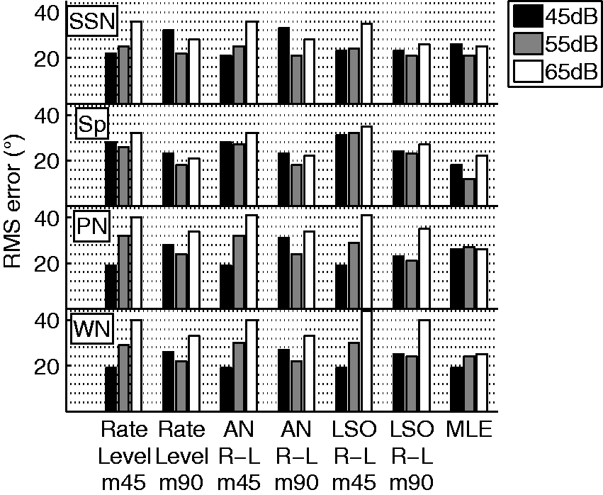
Despite their inherent differences, each model produced predictions that were within the range of published subject data (e.g., Grantham et al., 2007; Jones et al., 2014; Kerber & Seeber, 2012), thus making it difficult to say that one model is more realistic than the rest (Figure 11). It is also not possible to state which model is most accurate. What can be summarized from this subsection is that the LSO model is most robust against changes in signal level and that the MLE model performs best at the most lateral angles. Instead of choosing a model version based on performance, each one offers a different functional understanding of the input–output relations and should be chosen according to the focus of study.

Influence of the Test Stimulus

The best performing stimulus level, averaged over all stimulus types and prediction models, was 55 dB SPL with an RMS error of $23 . 6^{\circ} \pm 3 . 2^{\circ}$ (Figure 11, gray bars). This error is within the range of individual subject errors reported experimentally (e.g., Jones et al., 2014; Kerber & Seeber, 2012) and was approximately 5° better than the across-subject average. Model performance was comparable at 45 dB SPL and was somewhat worse at 65 dB, with RMS errors of $23 . 8^{\circ} \pm 5 . 3^{\circ}$ and $35 . 1^{\circ} \pm 3 . 9^{\circ}$ , respectively. Because the model was trained at 55 dB, it was not surprising that this level resulted in the best performance, especially considering that compression reduces the ICD for higher sound levels. Therefore, the azimuth was systematically underestimated at 65 dB, thus generating a larger error. At 45 dB, the opposite effect resulted in more lateralized estimates of the location. However, in the m45 case, there were systematically more underestimates at larger lateral angles, and the two effects largely canceled each other out, thus resulting in similar overall errors. The overall RMS error did not vary much when comparing the three different steady-state noise test stimuli (WN: $26 . 5^{\circ} \pm 8 . 0^{\circ}$ , SSN: $27 . 4^{\circ} \pm 6 . 0^{\circ}$ , and PN: $28 . 4^{\circ} \pm 6 . 7^{\circ}$ ). Although the model was trained with the SSN, slightly better performance was achieved with the frozen male speech segment ( $26 . 1^{\circ} \pm 5 . 0^{\circ}$ ). The intrinsic-level fluctuations that are inherent to speech resulted in a more linear rate-level function as opposed to the standard sigmoidal rate-level functions that were generated by the stationary stimuli (Figure 5). This linearity better appropriated the linear approximations made in the calibration step of the model and resulted in a lower mean RMS error. This result is also in line with subject data reported by Grantham et al. (2007) that showed a lower RMS error (reported as unsigned error) for similar 70 dB speech and white noise stimuli, $24 . 0^{\circ} \pm 10 . 1^{\circ}$ , $25 . 5^{\circ} \pm 9 . 6^{\circ}$ , respectively. This is an example where the model can offer an explanation behind an experimental finding. However, it must be noted that speech localization errors were smaller only for 16 of 22 subjects, a fact that further shows the need for individualizing the model to the CI subject.

In addition to testing the 4 different 200-ms stimuli in the absence of an interferer, data were also obtained for continuous speech (Figure 10, bottom row) and for a +5 dB signal-to-noise ratio condition (Figure 12). In the continuous speech, a new prediction was made every 200 ms, and the resulting large variability was caused by the nonstationary speech. Despite this variability, the distribution of predictions still retained the same basic bimodal form as that of the stationary stimulus. The central bias observed for more lateral angles in the +5 dB signal-to-noise ratio condition is in line with data for actual CI subjects (Kerber & Seeber, 2012) and can be explained by the reduction of ILD due to the 0-dB ILD of the interferer.

Figure 12.

Weighted average predictions and RMS error for clean SSN stimuli at 55 dB SPL (left) and the same stimuli at a signal-to-interferer ratio of +5 dB (right). The AN response difference localization model was used with the m90 slope calibration (same as Figure 9(a)).

Summary and Conclusions

A computer model for simulating the spatial hearing abilities of bilateral CI listeners was presented and tested in seven different versions. The model predictions were similar to the subjective performance of bilateral CI listeners not only in terms of the average localization error but also in the occurrence of systematic errors. The spatial resolvability of the model was too good, likely due to the absence of cognitive noise and due to modeling both ears with an identically programmed processor and an identical electrode-nerve interface. The different model versions performed fairly similar so that future studies should choose a version based on the focus of study. For studies investigating the origin along the processing chain, the two-stage rate-level model is recommended. For other purposes, the linear LSO rate-difference model is the best one-size-fits-all choice.

Irrespective of the particular version, the model confirmed a range of hypotheses from experimental studies, including the dominance of ILD cues in lateralization judgments, and the detrimental effect of level-dependent compression. The model allows for the identification of the origins of unexpected predictions along the processing chain. Beyond that, the proposed model of localization for bilateral CI can be useful in predicting performance of individual CI subjects by customizing the model to their clinical profile and for early stage testing of CI algorithms. It can be especially useful for the investigation of complex acoustic scenarios and more complex input systems (e.g., electro-acoustic stimulation or single-sided deaf), as well as in testing the influence of interaural pulse time differences at low pulse rates (with the ITD sensitive LSO model). From the investigations made to date, a binaurally coordinated n-of-m selection and compression are highly desirable for the next generation of CIs. Future model extensions are envisaged to include individualized versions of the processor setting, the electrode-nerve interface, and the mapping strategy.

Footnotes

Acknowledgments

We thank Tim Jürgens and Ben Williges for providing the code and support for the model, Le Wang for the LSO model code, Bernd Meyer for generating the multitalker speech-shaped noise, and Heath Jones for providing localization data of binaural CI subjects. We are indebted to David McAlpine, Volker Hohmann, and Nathan Spencer for valuable feedback on previous versions of the article. We are grateful to Birger Kollmeier and the Medical Physics group for continuous support and fruitful discussions.

Declaration of Conflicting Interests

The authors declared no potential conflicts of interest with respect to the research, authorship and/or publication of this article.

Funding

The authors disclosed receipt of the following financial support for the research, authorship, and/or publication of this article: The research leading to these results has received funding from the European Union’s Seventh Framework Programme (FP7/2007-2013) under ABCIT grant agreement n° 304912.

Note

References

Bingabr

Espinoza-Varas

Loizou

P. C.

(2008) Simulating the effect of spread of excitation in cochlear implants. Hearing Research 241(1): 73–79.

Chung

Delgutte

Colburn

H. S.

(2014) Modeling binaural responses in the auditory brainstem to electric stimulation of the auditory nerve. Journal of the Association for Research in Otolaryngology 16(1): 135–158.

Colburn

H. S.

Chung

Zhou

Brughera

(2009) Models of brainstem responses to bilateral electrical stimulation. Journal of the Association for Research in Otolaryngology 10(1): 91–110.

Day

M. L.

Delgutte

(2013) Decoding sound source location and separation using neural population activity patterns. The Journal of Neuroscience 33(40): 15837–15847.

Dietz

Ewert

S. D.

Hohmann

(2009) Lateralization of stimuli with independent fine-structure and envelope-based temporal disparities. The Journal of the Acoustical Society of America 125(3): 1622–1635.

Dietz

Ewert

S. D.

Hohmann

(2011) Auditory model based direction estimation of concurrent speakers from binaural signals. Speech Communication 53(5): 592–605.

Dorman

M. F.

Loiselle

Stohl

Yost

W. A.

Spahr

Brown

Cook

(2014) Interaural level differences and sound source localization for bilateral cochlear implant patients. Ear and Hearing 35(6): 633–640.

Duda

R. O.

Martens

W. L.

(1998) Range dependence of the response of a spherical head model. The Journal of the Acoustical Society of America 104(5): 3048–3058.

Faller

Merimaa

(2004) Source localization in complex listening situations: Selection of binaural cues based on interaural coherence. The Journal of the Acoustical Society of America 116(5): 3075–3089.

10.

Francart

MacDermott

(2012) Speech perception and localisation with SCORE bimodal: A loudness normalisation strategy for combined cochlear implant and hearing aid stimulation. PLoS One 7(10): e45385.

11.

Fredelake

Hohmann

(2012) Factors affecting predicted speech intelligibility with cochlear implants in an auditory model for electrical stimulation. Hearing Research 287(1): 76–90.

12.

Gerstner

Kistler

W. M.

(2002) Spiking neuron models: Single neurons, populations, plasticity, Cambridge, England: Cambridge University Press.

13.

Goupell

M. J.

Litovsky

R. Y.

(2014) The effect of interaural fluctuation rate on correlation change discrimination. Journal of the Association for Research in Otolaryngology 15(1): 115–129.

14.

Grantham

D. W.

Ashmead

D. H.

Ricketts

T. A.

Haynes

D. S.

Labadie

R. F.

(2008) Interaural time and level difference thresholds for acoustically presented signals in post-lingually deafened adults fitted with bilateral cochlear implants using CIS+ processing. Ear and Hearing 29(1): 33–44.

15.

Grantham

D. W.

Ashmead

D. H.

Ricketts

T. A.

Labadie

R. F.

Haynes

D. S.

(2007) Horizontal-plane localization of noise and speech signals by postlingually deafened adults fitted with bilateral cochlear implants. Ear and Hearing 28(4): 524–541.

16.

Greenwood

D. D.

(1990) A cochlear frequency-position function for several species—29 years later. The Journal of the Acoustical Society of America 87(6): 2592–2605.

17.

Hancock

K. E.

Delgutte

(2004) A physiologically based model of interaural time difference discrimination. The Journal of Neuroscience 24(32): 7110–7117.

18.

Hohmann

(2002) Frequency analysis and synthesis using a Gammatone filterbank. Acta Acustica united with Acustica 88(3): 433–442.

19.

Dietz

(2015) Comparison of interaural electrode pairing methods for bilateral cochlear implants. Trends in Hearing 19: 1–22.

20.

Imennov

N. S.

Rubinstein

J. T.

(2009) Stochastic population model for electrical stimulation of the auditory nerve. IEEE Trans Biomed Eng. 56(10): 2493–2501.

21.

Jones

Kan

Litovsky

R. Y.

(2014) Comparing sound localization deficits in bilateral cochlear-implant users and vocoder simulations with normal-hearing listeners. Trends in Hearing 18: 1–16.

22.

Kan

Stoelb

Litovsky

R. Y.

Goupell

M. J.

(2013) Effect of mismatched place-of-stimulation on binaural fusion and lateralization in bilateral cochlear-implant users. The Journal of the Acoustical Society of America 134(4): 2923–2936.

23.

Kayser

Ewert

S. D.

Anemüller

Rohdenburg

Hohmann

Kollmeier

(2009) Database of multichannel in-ear and behind-the-ear head-related and binaural room impulse responses. EURASIP Journal on Advances in Signal Processing 2009(1): 298605.

24.

Kerber

I. S.

Seeber

I. B. U.

(2012) Sound localization in noise by normal-hearing listeners and cochlear implant users. Ear and Hearing 33(4): 445–457.

25.

Laback

Pok

S. M.

Baumgartner

W. D.

Deutsch

W. A.

Schmid

(2004) Sensitivity to interaural level and envelope time differences of two bilateral cochlear implant listeners using clinical sound processors. Ear and Hearing 25(5): 488–500.

26.

Laneau, J. (2005). When the deaf listen to music–pitch perception with cochlear implants (Doctoral dissertation, Ph D dissertation). Katholieke Universiteit Leuven, Faculteit Toegepaste Wetenschappen, Leuven, Belgium.

27.

Litovsky

R. Y.

Goupell

M. J.

Godar

Grieco-Calub

Jones

G. L.

Garadat

S. N.

Misurelli

(2012) Studies on bilateral cochlear implants at the University of Wisconsin's Binaural Hearing and Speech Laboratory. Journal of the American Academy of Audiology 23(6): 476–494.

28.

Litovsky

R. Y.

Parkinson

Arcaroli

(2009) Spatial hearing and speech intelligibility in bilateral cochlear implant users. Ear and Hearing 30(4): 419–431.

29.

Macaulay

E. J.

Hartmann

W. M.

Rakerd

(2010) The acoustical bright spot and mislocalization of tones by human listener. The Journal of the Acoustical Society of America 127(3): 1440–1449.

30.

Majdak

Goupell

M. J.

Laback

(2011) Two-dimensional localization of virtual sound sources in cochlear-implant listeners. Ear and Hearing 32(2): 198–208.

31.

Majdak

Laback

Baumgartner

W. D.

(2006) Effects of interaural time differences in fine structure and envelope on lateral discrimination in electric hearing. The Journal of the Acoustical Society of America 120(4): 2190–2201.

32.

Mills

A. W.

(1958) On the minimum audible angle. The Journal of the Acoustical Society of America 30(4): 237–246.

33.

Nicoletti

Wirtz

Hemmert

(2013) Modeling sound localization with cochlear implants. In: Blauert

(ed.) The technology of binaural listening, Heidelberg, Berlin: Springer, pp. 309–331.

34.

Nopp

Schleich

D’haese

(2004) Sound localization in bilateral users of MED-EL COMBI 40/40+ cochlear implants. Ear and Hearing 25(3): 205–214.

35.

Potts

L. G.

Skinner

M. W.

Litovsky

R. A.

Strube

M. J.

Kuk

(2009) Recognition and localization of speech by adult cochlear implant recipients wearing a digital hearing aid in the nonimplanted ear (bimodal hearing). Journal of the American Academy of Audiology 20(6): 353.

36.

Remme

M. W.

Donato

Mikiel-Hunter

Ballestero

J. A.

Foster

Rinzel

McAlpine

(2014) Subthreshold resonance properties contribute to the efficient coding of auditory spatial cues. Proceedings of the National Academy of Sciences 111(22): E2339–E2348.

37.

Seeber

B. U.

Fastl

(2008) Localization cues with bilateral cochlear implants. The Journal of the Acoustical Society of America 123(2): 1030–1042.

38.

Spille

Dietz

Hohmann

Meyer

B. T.

(2013a, May) Using binaural processing for automatic speech recognition in multi-talker scenes. Paper presented at the Acoustics, Speech and Signal Processing (ICASSP), 2013 IEEE International Conference on, Vancouver, BC, Piscataway, NJ: IEEE, pp. 7805–7809.

39.

Spille

Meyer

B. T.

Dietz

Hohmann

(2013b) Binaural scene analysis with multidimensional statistical filters. In: Blauert

(ed.) The technology of binaural listening, Heidelberg, Berlin: Springer, pp. 145–170.

40.

Stadler

Leijon

(2009) Prediction of speech recognition in cochlear implant users by adapting auditory models to psychophysical data. EURASIP Journal on Advances in Signal Processing 2009: 5.

41.

Strutt

J. W.

(1907) On our perception of sound direction. Philosophical Magazine 13: 214–232.

42.

Swanson, B. A. (2008). Pitch perception with cochlear implants (PhD thesis). Faculty of Medicine, Dentistry & Health Sciences, Otolaryngology Eye and Ear Hospital, The University of Melbourne.

43.

Takanen

Santala

Pulkki

(2014) Visualization of functional count-comparison-based binaural auditory model output. Hearing Research 309: 147–163.

44.

Távora-Vieira

De Ceulaer

Govaerts

P. J.

Rajan

G. P.

(2015) Cochlear implantation improves localization ability in patients with unilateral deafness. Ear and Hearing 36(3): e93–e98.

45.

Tollin

D. J.

Yin

T. C.

(2002) The coding of spatial location by single units in the lateral superior olive of the cat. I. Spatial receptive fields in azimuth. The Journal of Neuroscience 22(4): 1454–1467.

46.

Tsai

J. J.

Koka

Tollin

D. J.

(2010) Varying overall sound intensity to the two ears impacts interaural level difference discrimination thresholds by single neurons in the lateral superior olive. Journal of Neurophysiology 103(2): 875–886.

47.

van Hoesel

Ramsden

O’Driscoll

(2002) Sound-direction identification, interaural time delay discrimination, and speech intelligibility advantages in noise for a bilateral cochlear implant user. Ear & Hearing 23(2): 137–149.

48.

van Hoesel

R. J.

Clark

G. M.

(1997) Psychophysical studies with two binaural cochlear implant subjects. The Journal of the Acoustical Society of America 102(1): 495–507.

49.

van Hoesel

R. J.

Tyler

R. S.

(2003) Speech perception, localization, and lateralization with bilateral cochlear implants. The Journal of the Acoustical Society of America 113(3): 1617–1630.

50.

Wagener

Kühnel

Kollmeier

(1999) Entwicklung und Evaluation eines Satztests für die deutsche Sprache I: Design des oldenburger satztests [Development and evaluation of a German sentence test part I: Design of the Oldenburg sentence test]. Zeitschrift für Audiologie/Audiological Acoustics 38(1): 4–15.

51.

Wang

Colburn

H. S.

(2012) A modeling study of the responses of the lateral superior olive to ipsilateral sinusoidally amplitude-modulated tones. Journal of the Association for Research in Otolaryngology 13(2): 249–267.

52.

Wang

Devore

Delgutte

Colburn

H. S.

(2014) Dual sensitivity of inferior colliculus neurons to ITD in the envelopes of high-frequency sounds: Experimental and modeling study. Journal of Neurophysiology 111(1): 164–181.

53.

Wierstorf

Raake

Spors

(2013) Binaural assessment of multichannel reproduction. In: Blauert

(ed.) The technology of binaural listening, Heidelberg, Berlin: Springer, pp. 255–278.

54.

Wightman

F. L.

Kistler

D. J.

(1992) The dominant role of low-frequency interaural time differences in sound localization. The Journal of the Acoustical Society of America 91(3): 1648–1661.

55.

Woodruff

Wang

(2013) Binaural detection, localization, and segregation in reverberant environments based on joint pitch and azimuth cues. Audio, Speech, and Language Processing, IEEE Transactions on 21(4): 806–815.

Auditory Model-Based Sound Direction Estimation With Bilateral Cochlear Implants

Abstract

Keywords

Introduction

Methods

Stimuli and HRTF Filtering

CI Processing

Electrode-Nerve Interface

AN Frequency Bands

Binaural Interaction Stage

Localization Models

Linear rate-level localization model

Linear response difference localization model

Maximum-likelihood estimation

Results and Discussion

Influence of the HRTF

Influence of the CI Processing

Influence of Spread of Excitation

Influence of the Binaural Model

Results of the Localization Models

Influence of the Test Stimulus

Summary and Conclusions

Footnotes

Acknowledgments

Declaration of Conflicting Interests

Funding

Note

References