Transmission of Binaural Cues by Bilateral Cochlear Implants: Examining the Impacts of Bilaterally Independent Spectral Peak-Picking,Pulse Timing,and Compression

Abstract

Acoustic hearing listeners use binaural cues—interaural time differences (ITDs) and interaural level differences (ILDs)—for localization and segregation of sound sources in the horizontal plane. Cochlear implant users now often receive two implants (bilateral cochlear implants [BiCIs]) rather than one, with the goal to provide access to these cues. However, BiCI listeners often experience difficulty with binaural tasks. Most BiCIs use independent sound processors at each ear; it has often been suggested that such independence may degrade the transmission of binaural cues, particularly ITDs. Here, we report empirical measurements of binaural cue transmission via BiCIs implementing a common “n-of-m” spectral peak-picking stimulation strategy. Measurements were completed for speech and nonspeech stimuli presented to an acoustic manikin “fitted” with BiCI sound processors. Electric outputs from the BiCIs and acoustic outputs from the manikin’s in-ear microphones were recorded simultaneously, enabling comparison of electric and acoustic binaural cues. For source locations away from the midline, BiCI binaural cues, particularly envelope ITD cues, were found to be degraded by asymmetric spectral peak-picking. In addition, pulse amplitude saturation due to nonlinear level mapping yielded smaller ILDs at higher presentation levels. Finally, while individual pulses conveyed a spurious “drifting” ITD, consistent with independent left and right processor clocks, such variation was not evident in transmitted envelope ITDs. Results point to avenues for improvement of BiCI technology and may prove useful in the interpretation of BiCI spatial hearing outcomes reported in prior and future studies.

Introduction

Disabling hearing loss impacts some 466 million individuals, roughly 5% of the global population (World Health Organization, 2020). Although most forms of hearing loss are permanent, technological solutions such as hearing aids can improve access to sound for the vast majority of affected individuals. For many individuals with severe to profound hearing loss, cochlear implants (CIs)—implanted neural prostheses that transform acoustic signals into sequences of electrical pulses—have proven remarkably successful in restoring access to sound and improving communication outcomes (Wilson & Dorman, 2008). However, despite success in tasks like speech understanding in quiet settings (which can be achieved with access to sound in one ear), success in other tasks such as speech understanding in noise and sound localization (which rely on input from two functional ears) has been limited for most CI users (e.g., J. G. W. Bernstein et al., 2016; Kan & Litovsky, 2015; Kerber & Seeber, 2012; Loizou et al., 2009; van Hoesel & Tyler, 2003).

The positioning of the ears on opposite sides of the head leads to differential acoustic delay and attenuation of sound arriving from sources in the environment, giving rise to interaural time difference (ITD) and interaural level difference (ILD) cues (e.g., Feddersen et al., 1957). These ITD and ILD cues aid in the localization of sound sources in the horizontal plane (Mills, 1958; Rayleigh, 1907) and in the perception and segregation of signals in noisy backgrounds (Cherry, 1953; Durlach, 1963), supporting spatial orientation, navigation, and communication (reviewed in Blauert, 1997; Litovsky et al., 2021). Normal-hearing (NH) listeners can detect ITDs as small as ∼10 μs (for low-frequency pure tones; Zwislocki & Feldman, 1956) and ILDs as small as ∼0.5 dB (across most of the audible spectrum; Mills, 1960).

Although NH listeners are not sensitive to ITDs conveyed by high-frequency (≥1500 Hz) temporal-fine-structure (the cycle-by-cycle fluctuations that define the waveform), listeners can be quite sensitive to ITDs conveyed by the envelopes of fluctuating high-frequency signals (Henning, 1974). For sufficiently slow (1–200 Hz) and prominent (high-modulation-depth) fluctuations, such envelope ITD sensitivity may approach that observed for low-frequency tones (Bernstein & Trahiotis, 2002). Notably, although NH individuals are thus able to access both ITDs and ILDs across frequency, ITDs carried by low-frequency signal components and stimulus onsets tend to dominate spatial judgments when available (Macpherson & Middlebrooks, 2002; Wightman & Kistler, 1992). Therefore, access to ITDs, and low-frequency ITDs in particular, is expected to be critical for typical spatial hearing abilities.

Toward restoration of access to binaural information and the associated perceptual binaural benefits described above, an increasing number of patients with severe to profound bilateral hearing loss have received bilateral CIs (BiCIs; Holder et al., 2018; Peters et al., 2010). Electrical stimulation via BiCIs provides demonstrable benefit over unilateral CI stimulation in many patients, for example, in terms of speech understanding in noise and sound localization; however, BiCI binaural outcomes remain highly variable and generally suboptimal, with binaural/spatial outcomes typically falling well short of NH performance (reviewed in Kan & Litovsky, 2015). Several factors may limit the binaural abilities of BiCI users; these can be grouped into device-related factors (e.g., technological limitations, surgical placement) and patient-related factors (e.g., constraints based on auditory system health, broadly defined; Kan & Litovsky, 2015). Here, we focus on a particular device-related factor: the fidelity of the transmitted ITDs and ILDs themselves.

Currently, most CI sound processors operate independently at each ear. Each device emits electrical pulses according to an internal clock, and pulse timing is not explicitly interaurally synchronized across devices (Laback et al., 2015; but see Bonnard et al., 2013). It has been suggested that a lack of interaural synchronization might disrupt or prevent the transmission of reliable ITDs (e.g., Grantham et al., 2007, 2008; Laback et al., 2004; Majdak et al., 2011; Potts et al., 2019). Although most CIs employ envelope-coding algorithms that replace the signal’s fine-structure with high-constant-rate pulse sequences that effectively eliminate temporal-fine-structure ITD (and exceed temporal rate limits on ITD sensitivity besides; e.g., van Hoesel et al., 2009), the pulses define the envelope, and variation in their timing could thus disrupt envelope ITDs as well.

Rodriguez and Goupell (2015) previously attempted to quantify transmission of envelope ITD (and ILD) cues via Cochlear N5 devices using the clinically widespread advanced combination encoder (ACE) sound processing strategy. The ACE strategy conveys information via a subset of available electrodes (“n-of-m,” typically 8 of 22 electrodes in modern devices), chosen on a running basis according to spectral peaks in the input signal. Rodriguez and Goupell recorded outputs from single electrodes of left and right “implants” worn by a binaural manikin. While recordings suggested that BiCI envelope ITD cues varied differently across azimuth than typical acoustic envelope ITDs, data were available for single channels only, and the source—or extent—of ITD distortion could not be determined.

Kan et al. (2018) followed the study of Rodriguez and Goupell (2015) with a carefully controlled set of multichannel recordings from Cochlear N6 devices also using ACE. Synthetic stimuli (30-Hz “transposed tones”) were delivered directly to the sound processors via direct line-in accessory ports with microphones disabled. Signals were first delivered to a single device to quantify the temporal variability of the resultant envelope across stimulus repetitions. Next, tones were filtered with left and right head-related transfer functions to render a spatialized binaural signal, and this signal was delivered to left and right sound processors and internal devices. Recordings collectively demonstrated that (a) variable pulse timing led to modest temporal jitter observable in the temporal envelope; (b) ITDs grew to larger than acoustic values at azimuths away from midline but generally followed a similar trajectory; and (c) independent spectral peak-picking in the two devices led to different channels being activated, effectively preventing ITD calculations on those channels.

In addition to possible disruptions of ITDs, processing elements such as nonlinear compression and automatic gain control (AGC) may distort ILDs transmitted by BiCIs (Archer-Boyd & Carlyon, 2019; Grantham et al., 2008; Kelvasa & Dietz, 2015; Litovsky et al., 2012; Potts et al., 2019). While ILD distortions are readily measured from hearing aids implementing similar compression algorithms (Brown et al., 2016; Wiggins & Seeber, 2011, 2012) and are readily predicted from BiCI simulations (Archer-Boyd & Carlyon, 2019; Dorman et al., 2014; Kelvasa & Dietz, 2015), few measurements have quantified such distortions as realized with actual CI sound processors responding to ecological stimuli.

In summary, despite a prevailing view that traditional BiCIs do not faithfully transmit binaural cues, relatively little empirical evidence (particularly in the case of ITDs) is available to quantify the incidence or extent of such. While BiCI spatial hearing benefit, however limited, is most commonly attributed to transmitted ILDs (Aronoff et al., 2010; Grantham et al., 2008; Kelvasa & Dietz, 2015), some evidence suggests that users can also access and benefit from transmitted ITDs while using clinical processors (including processors using the ACE coding strategy; e.g., Aronoff et al., 2010; Kerber & Seeber, 2013). To better parse limitations on the restoration of binaural hearing and associated benefits within the BiCI population, it is important to gain further insight on what binaural information BiCIs do or do not provide.

Here, we endeavored to quantify the transmission of ITD and ILD cues by a pair of modern CI sound processors (Cochlear N6) using the ACE coding strategy. Bilateral processors were worn by a binaural manikin positioned inside a hemi-anechoic chamber, with electrode outputs captured by a multichannel recording system. Measurements provide insight into fundamental limitations on access to binaural information ostensibly affecting many current BiCI users and point to possible avenues for improvement of BiCI technology.

Materials and Methods

Overview of the Basic Function of the CI Sound Processors

A CI consists of an external sound processor worn on the head (often behind the ear) and an implanted receiver-stimulator that relays the processed signal to an intracochlear electrode array (reviewed in Wilson & Dorman, 2008; Zeng et al., 2008). While some details of sound processor function are proprietary and manufacturer-specific, most commercial CI sound processing strategies include the same fundamental elements. The acoustic signal arriving at the external processor microphone(s) is divided, via bandpass filtering, into a number of parallel frequency channels. Within each channel, the temporal envelope of each bandpass-filtered signal is extracted and used to modulate the amplitude of sequences of electrical current pulses (“carrier pulse trains”; see below), which are sent by a receiver-stimulator to tonotopically organized electrodes along an intracochlear array. In some processors, including those used in the present investigation, the acoustic signal is passed through a “pre-emphasis” high-pass filter prior to bandpass filtering to augment the contribution of high-frequency signal components important in speech (Wilson & Dorman, 2008).

The carrier pulse trains that CIs use to elicit the sensation of sound typically consist of biphasic pulses delivered at a fixed rate (described in pulses per second [pps]). The process by which pulse trains are allocated to the electrodes defines the stimulation strategy. Spectral peak-picking, or “n-of-m,” stimulation strategies divide the amplitude spectrum into m contiguous frequency channels (based on the number of activated electrodes) and preferentially select the n most energetic channels for stimulation. This study used such a strategy (ACE). Another common stimulation strategy is to use uninterrupted pulse trains, in which there are no preferred channels and all electrodes (or a programmed subset, depending on the manufacturer) are constantly stimulated, provided that acoustic input is present above a set threshold (e.g., continuous interleaved sampling [CIS]; Wilson et al., 1991). CIS-like strategies were not evaluated in this study.

In an n-of-m strategy, the clinical pulse rate (pps) refers to the stimulation frame rate: The channel selection process occurs once per stimulation frame; within the frame period, n pulses are uniformly distributed in time across the n selected channels. Therefore, the true operating pulse rate of the implant is n times the clinical pulse rate (n × pps). Time is determined by an internal clock through the mechanical oscillations of a resonating crystal, the precise physical properties of which determine the exact pulse rate implemented. Slight variation in those properties may yield slight deviation from the nominal clinical pulse rate, potentially affecting relative timing across devices in the case of BiCIs (S. Duran, personal communication, September 18, 2020).

One basic task of an audiologist programming a CI sound processor is to map a range of acoustic input levels (in dB SPL) to a range of electrical current units that span the patient’s perceptual dynamic range from threshold to comfortable level (T-level to C-level, respectively, in Cochlear devices). Acoustic signals below the acoustic dynamic range are not transmitted, while acoustic signals above this range activate broadband AGC such that transmitted electrical current levels cease to increase beyond the C-level. CI level mapping is thus nonlinear and compressive as the dynamic range of electrical stimulation is less than the very broad range of possible acoustic input levels (e.g., Zeng et al., 2002). In practice, the acoustic dynamic range is defined in clinical software and further manipulated by adjusting the sound processor’s microphone sensitivity. While AGC thresholds can be raised by increasing the acoustic C-level and decreasing microphone sensitivity, AGC generally cannot be disabled in clinical devices. In modern sound processors, a variety of additional front-end processing features such as dynamic range processing, auditory scene classification, and noise reduction are often activated by default, subject to adjustment by the audiologist. Several such features were considered in this study, as described in the following section.

CI Sound Processors and Settings Used in the Present Study

All measurements of this study were completed using Nucleus 6, (i.e., N6) CP910 behind-the-ear sound processors (Cochlear Limited, Sydney, Australia). All sound processor settings were adjusted and verified using Custom Sound 5.2 software (Cochlear Limited). Processors used the ACE spectral peak-picking n-of-m strategy (described in detail earlier), with clinical default values of eight stimulating channels (n = 8) and all electrodes active (m = 22). The default clinical nominal pulse rate of 900 pps was used, giving an effective total rate of 7200 pps (assuming eight stimulated channels; note that sufficiently narrowband signals such as tones activate fewer channels). The duration of the positive and negative phases (phase duration) of each biphasic pulse was 50 µs, longer than the default 25 µs in order to facilitate better capture of pulse timing given the sampling frequency of our data acquisition system. Default intensity mapping and microphone sensitivity settings were used, resulting in acoustic T- and C-levels of 25 and 65 dB SPL, respectively. Corresponding electrical T- and C-levels (logarithmically related to acoustic T- and C-levels) were set to 50 and 200 current units across all 22 electrodes in both ears. This electric dynamic range was larger than what is typically used in real CI users but effectively served to improve the amplitude resolution of the recordings.

Stimuli (described later) were presented in four primary measurement sessions defined by four different CI program configurations, modified between sessions using Custom Sound. In Program A, for which the most extensive set of measurements was completed, all accessible processing algorithms were disabled (except AGC, which could not be), enabling assessment of the impact of bilateral device independence on binaural cues absent other impacts of additional front-end processing. In Program B, all default clinical settings/processing features on the Nucleus 6 CP910 processor were enabled. These included: “Adaptive Dynamic-Range Optimization” (ADRO), which uses slow, adaptive, channel-specific gain adjustments to increase gain in low-level channels and decrease gain in high-level channels, effectively performing spectral flattening; “Whisper,” which uses an additional dynamic range compression stage with make-up gain to effectively boost low-level signals; “autosensitivity control,” which uses signal-to-noise ratio (SNR) estimation to broadly reduce microphone sensitivity when noise levels exceed a certain threshold; “SCAN,” which classifies the auditory scene into one of the six scenes (quiet, speech, speech in noise, music, noise, and wind) and automatically activates appropriate front-end processing algorithms based on the classification; “WNR,” which reduces gain in channels classified as being dominated by wind noise; and “SNR-NR,” which reduces gain in channels classified as having a negative estimated SNR. (Note: More detailed descriptions of the processing features mentioned here are available in Wolfe et al., 2015 and in the Cochlear Limited Clinical Guidance Document, 2018). Program C was identical to Program B, except that SCAN was disabled, such that omnidirectional microphones were used (as in Program A). Program D was identical to Program B, except that ADRO was disabled. Measurements for Programs B to D were completed for a reduced set of stimuli, as described at relevant points in the “Results” section. All parameters not mentioned earlier were left at default values within Custom Sound, as follows: stimulation mode, MP1 + 2; channel gains, 0 dB for all; loudness growth, 20; volume, 6; soft MAP start duration, 0 s; and autosensitivity control threshold, 57 dB SPL.

Recording Hardware

Measurements were completed inside a hemi-anechoic chamber (HA-160, ETS-Lindgren Acoustic Systems, Cedar Park, TX), with additional floor treatment consisting of 19″ melamine wedges. Inside the chamber stood a circular array of 32 loudspeakers (Orb Mod1, Orb Audio, Sherman Oaks, CA), 13 of which were employed in this study. Loudspeakers were powered by 8-channel amplifiers (Crown CT 875, HARMAN Professional, Northridge, CA) connected to a 32-channel digital-to-analog converter (Orion 32, Antelope Audio, Sofia, Bulgaria). Utilized loudspeakers were located at 15° increments from −90° (left) to +90° (right) azimuth with respect to a binaural manikin (Knowles Electronic Manikin for Acoustic Research, GRAS Sound & Vibration A/S, Holte, Denmark) positioned on an adjustable stand at the center of the loudspeaker array. The manikin was aligned in the horizontal and vertical dimensions using a laser leveling system referenced to loudspeakers at 0°, +90°, and −90°.

CI sound processors were placed in the standard clinical position on the pinnae of the manikin (large pinnae, GRAS model KB0065/KB0066). Each processor was connected to a CI emulator (C124RE, Cochlear Limited) secured to the back of the manikin using Velcro. Data from 15 electrodes (E01–E10, E12, E14, E16, E18, and E20) were recorded from each ear/emulator. In Cochlear devices, Electrode 22 is the lowest frequency channel and 1 is the highest frequency channel. Left and right acoustic reference measurements were transduced via standard ½″ microphones (Type 40AO, GRAS) in the manikin’s ear canals, pre-amplified (Type 26CS, GRAS), and conditioned (Type 12AL, GRAS). Slight asymmetries in left- and right-ear acoustic outputs required post hoc correction, as described in following sections. For each ear, simultaneous electric and acoustic measurements (16 channels per ear) were combined via custom breakout boxes into two DB-25 balanced 8-channel cables (DBD-315, Hosa Technology, Inc., Buena Park, CA) and fed to a 32-channel analog-to-digital converter (Orion 32). The recording setup is illustrated schematically in Figure 1A, and an annotated frequency allocation table is given in Figure 1B.

Figure 1.

BiCI Recording Configuration. A: BiCI sound processors (Cochlear Nucleus 6 (N6) CP910) were placed on a KEMAR at the center of a loudspeaker array inside a hemi-anechoic chamber. Each sound processor was routed to an implant-in-a-box simulator (Cochlear CI24RE); the pulsatile outputs of both implant simulators—along with binaural acoustic signals from the manikin’s in-ear microphones—were captured simultaneously via a 32-channel ADC and recorded on a personal computer. B: Fifteen channels (out of 22) per device were recorded; each channel was defined by a lower (f1) and upper (f2) frequency boundary; recorded channels spanned a four-octave range, from approximately 500 to 8000 Hz. KEMAR = Knowles Electronic Manikin for Acoustic Research; ADC = analog-to-digital converter; CI = cochlear implant.

Software

Stimulus presentation and data acquisition were controlled via a graphical user interface programmed in MATLAB (R2018b, Mathworks, Natick, MA) running on a desktop computer. Analyses were conducted offline using MATLAB scripts that implemented standard signal processing techniques, as described at relevant points in the “Results” section.

Stimuli

Stimulus presentation levels were calibrated using a sound level meter (Type 2250, Brüel & Kjær Sound & Vibration Measurement A/S, Nærum, Denmark), paired with a ½″ microphone (Type 4189, Brüel & Kjær) placed in the center of the loudspeaker array on a tripod. Broadband noise (BBN), tones, and speech stimuli (Institute of Electrical and Electronics Engineers [IEEE] sentences; IEEE, 1969), sampled at 96000 Hz, were used (see Table 1). (Note: Additional stimuli were employed but offered conclusions redundant with those presented and are not treated in the present manuscript.)

Table 1.

Stimuli Used for Measurements of Binaural Cue Transmission via BiCIs.

Stimulus	Description
BBN	Bandwidth: 300 Hz to 8000 Hz; 1-s duration
Pure tone	fc = 500 Hz, 4375 Hz 1 s duration
SAM tone	fc = 500 Hz, 4375 Hz; fm = 10 Hz, 100 Hz; m = 100%; 1-s duration
CNC word	“Seek,” female talker; ∼1-s duration
Sentence	IEEE sentence, male talker; ∼3-s duration; 29.10: “Tight curls get limp on rainy days.”

Note. The sentence “Tight curls get limp on rainy days,” which is approximately 3 s in duration, was selected for its similarity to the average spectrum of sentences in the IEEE sentence database (IEEE, 1969); the CNC word “seek” was used as a brief speech token in a subset of measurements. BBN and pure-tone stimuli were generated with onset- and offset-ramps of 10 ms duration. f_c = carrier frequency; f_m = modulation frequency; m = modulation depth; IEEE = Institute of Electrical and Electronics Engineers; SAM = sinusoidally amplitude modulated; BBN = broadband noise; CNC = consonant-nucleus-consonant.

Acquisition Workflow

At the beginning of each data acquisition session, the acquisition system was initialized and the CI sound processors were loaded with new batteries. Batteries were replaced each session to ensure that devices received appropriate and constant power throughout the recording process.

Prior to testing a new processing configuration, the sound processors were removed from the manikin and connected to Custom Sound for reprogramming. Processors were then repositioned on the manikin as precisely as possible using landmarks on the pinnae as a guide.

Once playback and recording parameters were prepared for a specific stimulus configuration, stimulus presentation was initiated. Stimulus playback and recording were conducted one speaker location at a time, with eight stimulus repetitions per location. Stimuli were presented multiple times in order to provide for (a) estimation of trial-to-trial variability in the transmitted BiCI signals, and (b) denoising (via cross-trial averaging) of the binaural acoustic signal. In postprocessing, the acoustic recordings were averaged across stimulus repetitions to improve the SNR, and the BiCI recordings were gated to remove slight nonzero values attributable to between-channel crosstalk. An example of the basic signals obtained from one “ear” is provided in Figure 2. Analyses of the binaural information conveyed by the outputs of both implants, the ultimate objective of the present effort, are described in the following sections.

Figure 2.

Example Multichannel Recordings for One “Ear” for a Speech Sample (the IEEE Sentence “Tight curls get limp on rainy days”) Presented at 55 dBA. Upper and middle panels depict the waveform and spectrogram, respectively, of the acoustic signal as recorded in the in-ear microphone of a binaural manikin. The lower panel depicts the elicited CI electrodogram (note that pulses are biphasic but have been half-wave rectified for display). The CI was operating in Program A (see text).

Data Availability

Raw recordings files (absent all postprocessing described in the present manuscript) are available via the Open Science Framework (https://osf.io/8h2r9/) or via reasonable request submitted to the corresponding author.

Results

Independent Spectral Peak-Picking Leads to Interaurally Asymmetric Pulse Allocations

For any sound source away from the midline (0° azimuth), the signals reaching each ear are differentially impacted by interactions with the head, leading to interaural disparities in amplitude across frequency (i.e., frequency-dependent ILDs). In the case of acoustic signals, such interaural disparities reflect scaling along a continuum; the amplitude at one ear may be any nonzero multiple of the amplitude at the opposite ear within a given frequency band, but nonzero signal energy is present in both ears, enabling calculation of ILDs and phase-dependent ITDs. In the case of two CIs implementing spectral peak-picking independently, a fundamentally different kind of disparity can emerge: Within a given epoch, the two devices might select different sets of channels, such that for a given “binaural” channel (e.g., E04), pulses may be transmitted to only one ear. Figure 3A shows exemplar segments of left (blue) and right (red) outputs on electrode E04 elicited using BBN presented at 65 dBA from 0° azimuth (upper panel) and −90° azimuth (lower panel). The upper trace illustrates a case of symmetric pulse allocations—that is, a similar number of pulses transmitted by the left and right channel. In contrast, the lower trace of Figure 3A illustrates a case of highly asymmetric pulse allocation, with very few pulses occurring in the right channel despite a steady pulse sequence in the left channel. In this case, calculation of ILD is tenuous as the “binaural” signal is nearly unilateral (ILD values approach infinity), and ITD cannot be meaningfully calculated.

Figure 3.

Bilaterally Unsynchronized Spectral Peak-Picking Produces Asymmetric BiCI Outputs. Panels A to C show measurements for BBN presented at 65 dBA. A: Example recording segments from left (blue) and right (red) CI electrodes with high (upper panel) and low (lower panel) pulse-count symmetry (see text). B: Pulse distribution across the full stimulus duration for the left and right implants (left and right panels, respectively) as a function of azimuth and electrode. The number of pulses allocated to a given electrode at a given azimuth can differ substantially between devices (scale out of 1,000; the approximate maximum number of pulses possible per channel over the duration of a 1-s broadband noise is 900). C: BiCI pulse-count symmetry, expressed for each electrode at each azimuth as the percentage of pulses within a running 100-pulse-period window that occurred in both devices (100% indicates one-to-one correspondence; in other words, equal pulse count). The size of each square is scaled according to the effective average or RMS amplitude; in other words, the total number of left and right pulses for the given electrode/azimuth combination (compare with B). Data are averaged across positive and negative azimuths. D: Calculations as in B (inset) and C, but for a speech sample (“Tight curls get limp on rainy days”; see text). E: Pulse-count symmetry for three different stimuli and four presentation levels averaged across electrodes, and averaged again across eight stimulus repetitions, as a function of azimuth. Error bars represent ± SD across repetitions. All panels reflect recordings completed with devices using Program A.

Figure 3B illustrates pulse count (color intensity) across left and right electrodes (y-axes) as a function of azimuth (x-axes) for BBN presented at 65 dBA. At the midline, where impinging left and right signals are maximally symmetric (not differentially affected by the head), most pulses are allocated to electrodes E12–E02 in both devices (corresponding to frequencies between approximately 1.5 and 7 kHz). However, at source azimuths increasingly contralateral to a given device (e.g., +75° or +90° for the left device), high-frequency signal components are attenuated by the head, and pulses are thus increasingly allocated to lower frequency channels. Meanwhile, pulse allocations in the device ipsilateral to the source change only slightly. The degree of resultant symmetry can be quantified according to the number of pulses that occur in both versus only one ear. Here, we quantify symmetry within a running 100-pulse-period temporal window (∼110 ms duration, given the 900 pps clinical pulse rate) with 50% overlap: A symmetry value of 100 means that the pulse count was equal across the ears, while a symmetry value of 0 means that the pulses were allocated to only one ear (i.e., completely asymmetric). As the amplitude and number of total pulses can vary both across windows within a given channel and in total across channels, the time-averaged symmetry is calculated from the weighted mean symmetry across windows, with weights according to root-mean-square (RMS) energy per window. As anticipated from Figure 3B and quantified in Figure 3C, symmetry generally decreases with increasing azimuth, particularly for apical and basal electrodes.

While BBN is a tractable synthetic stimulus that can elicit output from all electrodes, CIs are built primarily to process speech, and analyses based on spectrotemporally random (long-term spectrally “flat”) noise may point to results of limited ecological importance. Therefore, the symmetry analysis was next applied to a sentence (“Tight curls get limp on rainy days”) spoken by a male talker presented at a soft conversational level of 55 dBA (see also Table 1 and Figure 2). As shown in Figure 3D, the allocation of pulses across electrodes is rather different than for BBN due to the prominent spectral peaks in speech, including a prominent low-frequency peak (e.g., E20 and E18). However, results are qualitatively similar to those for BBN, in that symmetry values in most channels are relatively high near 0° azimuth, but greatly reduced at larger azimuths, particularly at high frequencies.

Figure 3E summarizes pulse-count asymmetry measurements for BBN and two different speech stimuli (the sentence in Figure 3D and the consonant-nucleus-consonant word “seek,” spoken by a female talker; see Table 1). Cross-electrode weighted-average asymmetry values are plotted as a function of azimuth at four different presentation levels (35–65 dBA, panels as labeled). Notably, in addition to azimuth effects already discussed, symmetry worsens with decreasing stimulus amplitude. At large azimuths in particular, head-shadow effects act on the already-low source level to bring many signal segments/frequency bands below programmed device T-levels, leading to the omission of pulses in the contralateral device. Correspondingly, an analysis of variance of symmetry transformed to logits revealed main effects of source azimuth, F(6, 588) $=59\text{,}282.27$ , $p<.001$ , ${\mathrm{\eta }}^2=.47$ , stimulus level, F(3, 588) $\mathrm{\hspace{0.17em}}=83\text{,}236.62$ , $p<.001$ , ${\mathrm{\eta }}^2=.33$ , and stimulus type, F(2, 588) $\mathrm{\hspace{0.17em}}=51\text{,}042.75$ , $p<.001$ , ${\mathrm{\eta }}^2=.13$ . The interactions of azimuth and level, F(18, 588) $=387.75$ , $p<.001$ , ${\mathrm{\eta }}^2=.01$ , azimuth and stimulus type, F(12, 588) $=592.26$ , $p<.001$ , ${\mathrm{\eta }}^2=.01$ , stimulus type and level, F(6, 588 ) $=5\text{,}440.32$ , $p<.001$ , ${\mathrm{\eta }}^2=.04$ , and the three-way interaction, F(36, 588) $\mathrm{\hspace{0.17em}}=188.69$ , $p<.001$ , ${\mathrm{\eta }}^2=.01$ , were all significant, highlighting the complex spatially dependent nature of cross-electrode average symmetry. In general, speech stimuli resulted in somewhat poorer symmetry than BBN at lower presentation levels. Tukey honestly significant difference post hoc comparisons within the level and type dimensions revealed no significant difference between the two speech stimuli (“word” and “sentence,” $p>.05$ ) but significantly lower symmetry for both speech stimuli than for BBN ( $p<.05$ for both comparisons) at 35 and 45 dBA. At 55 dBA, there was no significant difference between “word” and “sentence” ( $p>.05$ ) or “sentence” and “BBN” ( $p>.05$ ), but the significant difference between “word” and “BBN” persisted ( $p<.05$ ). At 65 dBA, symmetry values were similar across stimuli ( $p>.05$ for all; note convergence of plots in the rightmost panel of Figure 3E).

In summary, interaurally independent peak-picking can lead to substantially asymmetric signals across the ears. As will be shown in the following sections, such asymmetry fundamentally constrains and generally degrades the transmission of binaural cues (and complicates their definition). Notably, this constraint is independent of, and more severe than, impacts of independent pulse timing or gain control per se (cf. Kan et al., 2018; see “General Discussion” section).

BiCI Transmission of ILD and ITD Cues Conveyed via BBN at a Fixed Level

Recognizing fundamental constraints on the transmission of binaural information expected due to left–right channel asymmetries described earlier, we next proceeded to quantify BiCI binaural cue transmission. Cues were quantified across the stimulus types and presentation levels provided in Table 1. We begin with the case of BBN presented at 65 dBA. ILDs (in dB) were computed by comparing the RMS amplitudes of the left and right signals according to the standard formulation,

$$\mathrm{ILD}=20{\log }_{10}\left(\frac{\sqrt{\frac{1}{T}{\int }_0^T{x}_R^{\mathrm{\hspace{0.17em}}2}\left(t\right)\mathrm{d}t}}{\sqrt{\frac{1}{T}{\int }_0^T{x}_{\mathrm{L}}^{\mathrm{\hspace{0.17em}}2}\left(t\right)\mathrm{d}t}}\right)$$

(1)where the numerator and denominator yield the RMS of the right-ear (x_R) and left-ear (x_L) signals, respectively. By construction, larger amplitudes in the right ear lead to ILD > 0 dB and larger amplitudes in the left ear lead to ILD < 0 dB. Note that ILD values reflect natural sound pressure levels in the case of the acoustic recordings, and programmed current levels in the case of the CI recordings, and are thus not directly comparable.

ITDs were quantified according to the delay at the maximum of the function given by cross-correlation of left and right signals,

$$\mathrm{\gamma }\left(\mathrm{\tau }\right)=\frac{{\int }_0^T{x}_L\left(t\right)x_R(t+\mathrm{\tau })\text{d}t}{\sqrt{{\int }_0^T{x}_L^{\mathrm{\hspace{0.17em}}2}\left(t\right)x_R^{\mathrm{\hspace{0.17em}}2}(t+\mathrm{\tau })\text{d}t}}$$

(2)where τ defines the relative delay between the left- and right-ear signals; τ was limited to the range −2,500 ≤ τ ≤ 2,500 µs. Calculations were completed in a “narrowband” sense using bandpass-filtered signals (filter cutoff frequencies matched to the frequency allocation table shown in Figure 1B) or single-electrode outputs. Where indicated, “broadband” estimates were obtained by calculating a weighted-average (according to channel RMS) of the “narrowband” values. Waveform ITDs were derived from left and right waveforms (acoustic) or pulse sequences (CI), while envelope ITDs were calculated using the low-pass-filtered (150-Hz cutoff) Hilbert envelope of each.

Slight physical imperfections of the acoustic manikin and its placement in the speaker array, imperfect placement of the CI sound processors, and differences in microphone transfer functions can all cause nonzero binaural cues at 0° azimuth. In the data that follow, functions with near-zero artifactual offsets at 0° were corrected to zero (e.g., a +20-µs ITD or +2-dB ILD at 0° would lead to subtraction of 20 µs or 2 dB from the respective cross-azimuth function), while functions were left uncentered if the offset at 0° azimuth was large (e.g., see Figure 4B, upper panel). “Slipped” cycles in ITDs conveyed by CI pulse sequences were detected by identifying changes across adjacent azimuths greater than 50% of the CI pulse period and corrected by shifting slipped values toward the real values by integer multiples of the pulse period.

Figure 4.

Acoustic and Electric Binaural Cues Calculated From Recordings of BBN at 65 dBA. A: (Upper panel) Broadband ILD calculated across eight stimulus repetitions using the broadband left- and right-ear waveforms (acoustic; black) or the cross-channel sum of left- and right-implant electrode outputs (CI, red). *Note that units of acoustic and electric (CI) ILDs should not be directly compared (see text). (Middle panel) Narrowband acoustic ILD calculated after filtering the broadband waveforms with bandpass filters matched to electrode frequencies, as labeled; see also Figure 1B. The size of each point is weighted by the average RMS amplitude of left and right channels at the corresponding azimuth. (Lower panel) Electrode-specific electric ILDs, as labeled. X symbols denote instances in which one channel (left or right) conveyed no pulses (0% symmetry) for between one and seven of the eight stimulus repetitions. Downward arrows near the bottom of a subpanel denote instances in which all stimulus repetitions elicited output in the left device only. B: (Upper panel) Broadband “waveform” ITD calculated via weighted averaging of channel-specific cross-correlation values (see text) using left- and right-ear waveforms (acoustic, black) or left- and right-implant electrode outputs (CI, red). (Middle panel) Narrowband waveform ITD; points/symbols as in A. (Lower panel) Electrode-specific ITD. C: (Upper panel) Broadband envelope ITD calculated as for waveform ITD but using the low-pass-filtered Hilbert envelope (see text) of the left-and right-ear waveforms (acoustic, black) or left- and right-implant electrode outputs (CI, red). (Middle panel) Narrowband envelope ITD; points/symbols as in A. (Lower panel) Electrode-specific envelope ITD. All panels reflect recordings completed with devices using Program A. ITD = interaural time difference; ILD = interaural level difference.

Figure 4A plots ILD across azimuth (0°–90°). The upper panel displays broadband calculations for acoustic signals (black circles) and BiCI outputs (red squares). We reiterate that the “ILD” associated with electrical stimulation, which is effectively an index of the interaural difference in current provided to auditory nerve fibers, should not be directly compared with acoustic (conventional) ILD, which is an index of the level difference in the acoustic signals reaching the two ears. Nonetheless, the trajectory of BiCI ILD prominently diverged from that of the acoustic ILD with increasing azimuth, a matter explored further in the next subsection.

Middle and lower panels of Figure 4A plot narrowband acoustic and single-electrode BiCI ILDs, respectively. Within each panel, colors give data for 15 different frequency bands (acoustic data obtained by digitally bandpass-filtering broadband acoustic data using a bank of sixth-order, zero-phase Butterworth filters with pass bands matched to corresponding electrode frequencies), and the size of each point is weighted according to the summed left and right RMS level (average of x_R and x_L in Equation 1) for the given frequency-azimuth combination. Acoustic ILDs exhibit the expected trajectory (e.g., Feddersen et al., 1957), with a steady increase in ILD magnitude with increasing frequency, and modest nonmonotonicity across azimuth in the mid-frequency region (approximately 1500–3000 Hz) associated with the “acoustical bright spot” (e.g., Macaulay et al., 2010; Mayo & Goupell, 2020). The cross-electrode pattern for BiCI ILDs was notably different. Despite the broadband nature of the signal, very few pulses were transmitted in low-frequency channels, and there was a tendency for the lowest frequency channels to yield negative ILDs, even infinite negative ILDs (red downward arrows), occurring when the CI ipsilateral to the source emitted no pulses. This pattern apparently arose due to the asymmetry issue delineated in the preceding subsection: For a spectrally “flat” source signal such as BBN arriving from sources away from the midline, pulses at the ipsilateral CI are allocated primarily to high-frequency channels (owing to pre-emphasis filtering), while at the contralateral CI, high-frequency energy is substantially attenuated by the head shadow. Therefore, (a) low-frequency channels are more likely to get picked in the contralateral device, leading to spurious negative ILDs in those channels, while (b) high-frequency channels are more likely to get picked in the ipsilateral device, leading to very large positive ILDs in those channels. At the level of 65 dBA illustrated in Figure 4A, these effects are modest; more dramatic effects (and a higher incidence of “infinite” ILDs, including infinite positive ILDs) can be observed at lower presentation levels (see following subsection).

Regarding ITDs, Figure 4B plots “waveform” acoustic and electric ITDs across azimuth. Values in the upper panel again reflect “broadband” acoustic (black circles) and BiCI (red squares) data. Middle and lower panels again show frequency-specific values with points weighted according to the average of left and right RMS levels, generally in agreement with the broadband values. Acoustic values follow the expected trajectory, increasing monotonically with azimuth to a maximum of approximately 700 µs at +90°. BiCI values are quite different: Although increasing with azimuth similar to acoustic ITD, the BiCI value at 0° azimuth is 400 µs. As will be demonstrated in a subsequent section, this value is due to the arbitrary relative timing of pulses from the two CIs, each operating on its own clock; had one processor been turned on at a slightly different time, the y-value of the entire function could be shifted by hundreds of microseconds in either direction.

Figure 4C plots acoustic and electric envelope ITDs. Broadband (upper panel) acoustic values again generally follow the expected trend, reaching a maximum slightly more than 700 µs at +90°. Narrowband acoustic envelope ITDs fluctuated in the low-frequency region, owing to relatively low signal energy and a sparsely defined envelope given the relatively low center frequencies. Interestingly, in the mid-frequency region, narrowband acoustic values of envelope ITD featured an unexpectedly nonmonotonic trajectory across azimuth. Further analysis established that this was not a measurement artifact, but true nonmonotonicity in narrowband envelope ITDs, reproduced with several publicly available databases (e.g., Kayser et al., 2009; data not shown). At higher frequencies, improved SNR (due in part to ear canal resonance) and a well-defined envelope yielded cross-azimuth envelope ITD functions similar to the broadband estimate.

BiCI envelope ITD values increased with increasing azimuth in a manner qualitatively similar to acoustic ITDs. Cross-electrode averaged BiCI ITDs closely followed cross-frequency average acoustic ITDs (Figure 4C, upper panel). However, electrode-specific envelope ITDs (Figure 4C, bottom panel) fluctuated across azimuth and frequency, particularly at +90°, where ITDs in excess of 2,000 µs were computed for both E03 and E04 (note that “slipped cycle” corrections do not apply to envelope ITDs). Examination of the channel-specific envelopes confirmed influences of left–right pulse asymmetry: Whereas acoustic envelope differences at the two ears depended only on acoustic travel (delay) and head-shadow (scaling) effects, BiCI envelope differences were impacted by these effects in combination with sporadic, interaurally independent fluctuations due to asymmetric pulse allocations. Given asymmetric allocation of pulses between left and right CIs within a given channel, left and right envelopes are no longer related by a simple azimuth-dependent time-shifting/scaling function. Spurious ITDs and nonmonotonic ITD-versus-azimuth functions can result. Nonetheless, it is notable that independent clinical BiCIs transmitted a broadband cross-azimuth envelope ITD function of a generally monotonic form similar to that observed acoustically.

Level Dependence of ILD and Envelope ITD Transmission for Noise and Speech Stimuli

To examine BiCI transmission of binaural cues across a broader range of stimulus features, we next quantified BiCI ILDs and ITDs for both BBN and speech across several stimulus presentation levels. Figure 5A plots ILDs (upper row) and envelope ITDs (lower row) for BBN presented at five different levels (25–65 dBA). Cues were calculated in a “narrowband” sense (i.e., for each electrode; organization and colors as in the lower panels of Figure 4A and C).

Figure 5.

BiCI ILDs and Envelope ITDs as a Function of Azimuth Across Presentation Levels. (Color legend as in Figure 4) A: BBN was presented at five different levels (25–65 dBA in 10-dB steps). ILDs (top row) were calculated within-electrode channels. Each stimulus (azimuth-by-level combination) was presented 8 times. Due to asymmetric spectral peak-picking, sometimes only one device (left or right) generated pulses for a given channel. X symbols denote instances in which such asymmetry occurred for between one and seven of the eight stimulus repetitions. Upward arrows near the top of a subpanel denote instances in which all stimulus repetitions elicited output in the right device only, while downward arrows near the bottom of a subpanel denote instances in which all stimulus repetitions elicited output in the left device only. Envelope ITDs (bottom row) were calculated as in Figure 4 and are displayed using the same symbol conventions used for ILDs. The solid black line denotes the broadband acoustic envelope ITD (from Figure 4C, upper panel). B: As in A, but for the IEEE sentence “Tight curls get limp on rainy days.” All panels reflect recordings completed with devices using Program A. ITD = interaural time difference; ILD = interaural level difference.

A profound impact of presentation level on transmitted ILDs was evident: ILDs systematically decreased with increasing presentation level. This result is expected (see “Introduction” section) and attributable to nonlinear level mapping (compression and AGC). The form of the function elicited at specific presentation levels depends on the stimulus and on the programmed level settings (we used clinically typical settings, see “Materials and Methods” section) but may be understood in a general sense as follows: At “low” presentation levels, the output of each device scales with the acoustic input level, which increases slightly with increasing azimuth at the ipsilateral CI and decreases substantially at the contralateral CI due to the acoustic head shadow, resulting in relatively large ILDs at large azimuths. At sufficiently low presentation levels and in sufficiently high-frequency channels for which the acoustic head shadow is most effective, the sound level reaching the contralateral CI can drop below the programmed T-level, resulting in zero pulses from the contralateral CI and an infinite positive ILD (upward triangles in Figure 5A). With increasing presentation level, the output from the ipsilateral CI is increasingly limited by compression, and the ILD is primarily impacted by changing level at the contralateral CI, which remains in a relatively more linear regime due to the impact of the head shadow. At sufficiently high levels, output levels for both ipsilateral and contralateral devices begin to saturate, reducing ILDs toward 0 dB. Finally, as described in the preceding subsection, negative ILDs (and even infinite negative ILDs, downward triangles in Figure 5A) can occasionally occur due to pulse allocation asymmetry in the lowest frequency channels favoring the ear contralateral to the sound source.

An impact of presentation level on envelope ITD transmission is also evident (Figure 5A, lower row), though the effect was less pronounced than that for ILD. While calculated values at each presentation level generally trended upward with increasing azimuth (broadband acoustic values are provided for reference, black line), cross-electrode and cross-azimuth variability increased somewhat at low presentation levels. We attribute this result to increased pulse allocation asymmetry at low levels (as shown in Figure 3E; see following subsection). At the lower presentation levels and particularly in the higher frequency channels (due to head-shadow effects described in the preceding paragraph), fully asymmetric outputs sometimes occurred (zero pulses in a given channel), preventing calculation of a meaningful ITD (upward and downward triangles).

As with the calculation of pulse asymmetry itself (Figure 3), caveats regarding the use of noise to interrogate a device built to process speech certainly apply to binaural cue calculation. Therefore, the calculations of Figure 5A were repeated using the sentence stimulus considered in Figures 2 and 3. Resultant cues (Figure 5B) generally resembled those for noise (Figure 5A) with a few differences. ILD magnitudes (top row) once again decreased with increasing presentation level but maintained a more organized pattern across frequency at each presentation level. Owing to the relatively higher signal energy of the speech signal in the low-frequency channels (and the consequently higher pulse-count symmetry; see Figure 3D), negative ILDs did not occur here as they did for noise, even at the lowest presentation levels. At the highest presentation levels, ILDs for speech were somewhat larger than for noise, ostensibly owing to the more dynamic nature of the speech envelope which reduced the impact of level saturation (a matter considered in the context of dynamic ILDs in a subsequent section). Envelope ITDs conveyed by speech followed the same general pattern as those conveyed by noise, but were greatly impacted by pulse allocation asymmetry at the lowest levels, a result anticipated from the significantly greater asymmetry observed for speech than spectrally flat noise (see preceding section, Figure 3). Supraphysiologic ITDs (≳1 ms for the human head) still occurred even at the highest levels for the high-frequency electrodes, again a product of persistent asymmetry. We next considered the impact of asymmetry on ILD and envelope ITD variability explicitly.

Pulse-Count Asymmetry Increases the Variability of ILD and Envelope ITD Transmission

It was previously noted that pulse-count asymmetry tended to increase with sound-source azimuth (see Figure 3). As azimuth is also the parameter onto which ILD and ITD values must be “mapped” for spatial hearing benefit, it is useful to further parse the impacts of pulse-count symmetry and azimuth on BiCI-transmitted ILD and envelope ITD cues. Here, we specifically focus on the relationships among pulse-count asymmetry, source azimuth, and the cross-trial variability of transmitted ILD and ITD cues, which fundamentally limits the precision with which these cues may be related to azimuth.

Figure 6A plots symmetry (in logits) versus azimuth, per trial, for all BBN and speech presentations for Program A at all presentation levels. Data are shown for all electrodes (colors as in Figure 4). While there was an apparent tendency for lower pulse-count symmetry to occur at larger azimuths, any pair of electrodes could exhibit low symmetry (<1 logit or approximately 75% symmetry) at nearly any azimuth. In instances where low symmetry occurred, the variability (standard deviation [SD] across repetitions) of transmitted ILD and envelope ITD values for the corresponding azimuth–electrode pair combination tended to be large. Figure 6B plots SD of ILD cues (in dB) across repetitions versus mean pulse-count symmetry (in logits). Figure 6C plots SD of envelope ITD cues (in dB) across repetitions versus mean pulse-count symmetry (in logits). For reference, an approximation of a “good” BiCI psychophysical ITD threshold obtained with 1,000-pps stimuli under ideal conditions is given by the dashed line (approximated from Noel & Eddington, 2013, Figure 4, 100-Hz amplitude modulation condition). A similar reference for ILD would require additional assumptions not treated here.

Figure 6.

Effect of Pulse-Count Symmetry on the Variability of Binaural Cues. (Color legend as in Figure 4) A: Pulse-count symmetry in logits as a function of azimuth pooled across noise and speech stimuli. Multiple linear regression revealed that the interaction of azimuth and symmetry was not significant for both envelope ITD variability and ILD variability across repetitions. While symmetry tends to decrease with increasing azimuth, low symmetry can occur for any electrode at any azimuth, resulting in a weak relationship between azimuth and cue variability. B: SD of BiCI ILDs across repetitions as a function of mean pulse-count symmetry in logits. C: SD of BiCI envelope ITDs across repetitions as a function of mean pulse-count symmetry in logits. The dashed line at y = 100 µs approximates a “good” threshold ITD obtained at 1,000 pps under direct stimulation, for which clinical processor-related variability is eliminated (from Noel & Eddington, 2013; see text). All panels reflect recordings completed with devices using Program A. ILD = interaural level difference; ITD = interaural time difference; SD=standard deviation.

To parse the sources of observed cue variability, we performed two multiple linear regressions on the explanatory variables of azimuth, mean symmetry (across repetitions), presentation level, electrode pair, and stimulus (coded categorically relative to BBN). The response variables in the two analyses were SD of ILD across repetitions, and SD of envelope ITD across repetitions. In these models, response variables were weighted proportional to signal energy.

These analyses revealed the following relationships to be significant: For ILD variability, F(16, 1075) $\mathrm{\hspace{0.17em}}=277.15$ , R² _adj $\mathrm{\hspace{0.17em}}=.72$ , $p<.001$ , significant predictors included mean symmetry ( $\mathrm{\beta }=-.391,\mathrm{\hspace{0.17em}}p<.001$ ), presentation level ( $\mathrm{\beta }=-.018,\mathrm{\hspace{0.17em}}p<.001$ ), and stimulus type (per categorical coding, both “word,” $\mathrm{\beta }=.020,\mathrm{\hspace{0.17em}}p<.001$ , and “sentence,” $\mathrm{\beta }=.018,\mathrm{\hspace{0.17em}}p<.001$ , yielded positive coefficients, indicating greater cue variability for speech stimuli relative to BBN, cf. Figure 3E). For envelope ITD variability, F(16, 1075) $\mathrm{\hspace{0.17em}}=189.4$ , R² _adj $\mathrm{\hspace{0.17em}}=.61$ , $p<.001$ , significant predictors included mean symmetry ( $\mathrm{\beta }=-.289,\mathrm{\hspace{0.17em}}p<.001$ ), presentation level ( $\mathrm{\beta }=-.015,\mathrm{\hspace{0.17em}}p<.001$ ), stimulus type (“word,” $\mathrm{\hspace{0.17em}}\mathrm{\beta }=.311,\mathrm{\hspace{0.17em}}p<.001$ , “sentence,” $\mathrm{\beta }=.111,\mathrm{\hspace{0.17em}}p<.001$ ), and the interaction of symmetry and level ( $\mathrm{\beta }=.003,\mathrm{\hspace{0.17em}}p<.001$ ). Notably, neither azimuth nor electrode were significant predictors of cue variability in either model ( $p>.05$ for all). The negative model coefficients for symmetry and level indicate that binaural cue variability decreased with increasing symmetry or presentation level (which tended to covary, i.e., higher presentation levels led to higher symmetry; see Figure 3E). In summary, low symmetry could happen at any azimuth or electrode (particularly for speech and low signal levels) and, wherever it occurred, resulted in high within-electrode binaural cue variability.

Pulse-Timing “Drift” and the Minimal Effect of Unsynchronized Processor Clocks on Envelope ITDs

Clinical BiCI processors are unsynchronized, with independent clocks that (a) are likely to carry an arbitrary relative temporal offset depending on when each device was turned on and (b) may also implement slightly different exact pulse rates (see “Materials and Methods” section). As described in the “Introduction” section, it has often been suggested that this lack of synchronization might corrupt the transmission of useful ITD information. Here, we examine this possibility explicitly.

One simple means to evaluate the reliability of pulse-timing-based ITD is to calculate the ITD at a constant azimuth across a series of measurement sessions. To this end, Figure 7A shows pulse-timing ITD for sinusoidally amplitude modulated (SAM) and pure-tone stimuli presented at 0° azimuth—for which the acoustic ITD is always ∼0 µs. Data are plotted as a function of time (in hours) across several days (panels) of recording. To maximize the number of data points available, recordings for these stimuli for all Programs A to D were evaluated (colors, as labeled). ITD calculations were made (using Equation 2) for the pulse trains recorded from the electrodes centered at the tone (or SAM tone carrier) frequency (E20 and E5 for 500 Hz and 4375 Hz stimuli, respectively). The resulting ITD values were “wrapped” to the pulse period,

$$\text{IT}{\text{D}}_{\text{wrapped}}\mathrm{\hspace{0.17em}}=\mathrm{\hspace{0.17em}}\mathrm{mod}(\mathrm{ITD}+\frac{T_{\mathrm{CI}}}{2},\mathrm{\hspace{0.17em}}{T}_{\mathrm{CI}})-\frac{T_{\mathrm{CI}}}{2}$$

(3)where $T_{\mathrm{CI}}$ represents the pulse period (1/pps) and $\mathrm{mod}\left(\right)$ represents the modulo operator.

Figure 7.

Pulse-Timing ITD Is Arbitrary But Minimally Affects Envelope ITDs. A: “Waveform” ITD based on timing of discrete electrical pulses wrapped to the ∼550-µs pulse period for all SAM and pure-tone stimuli at 0˚ azimuth as a function of time of recording. Recordings occurred across several days (panels). Preprocessing program is denoted by color. Pulse-timing ITD varied widely at a constant (0˚) azimuth and is thus an unreliable cue for source azimuth. B: Pulse-timing ITD (left panel) and envelope ITD (right panel) calculated from whole waveforms as a function of azimuth for multiple restarts of the left sound processor (colors). Each restart placed the CI pulse trains in some new relative alignment with each-other, shifting the y-intercept of the “waveform” ITD-azimuth function. However, processor restart minimally affected envelope ITDs. C: Same as in B, but calculated using a 50-ms window containing the transient “/k/” in the stimulus “seek”. Processor restart arbitrarily affected the y-intercepts of “waveform” ITD-azimuth functions, similar to whole-waveform effects. Transient envelope ITDs were impacted by a different issue—missing pulses that prominently impacted the transient envelope cross-correlation, yielding average ITDs near 0 in many cases (see text). ITD = interaural time difference; CI = cochlear implant.

Despite the constant 0° source azimuth, the pulse-timing-based ITD varied widely as a function of time. ITDs repeatedly traversed the entire pulse period, approximating a periodic sawtooth function (allowing for inhomogeneous sampling due to irregularity of recording session times). Nearly overlapping data points are ITDs for each of the eight repetitions of each given stimulus, completed within a short period relative to the overall time scale represented. However, even over this brief period, the “drift” in calculated ITDs is evident. Calculated across recordings, the estimated drift rate for the specific processors used in the present study is ∼0.005 Hz, or one cycle per ∼3.3 min. Due to the continuously varying relationship of left and right pulse timing, any ITD—when calculated on the basis of individual pulse timing—could occur at 0° azimuth. Data therefore suggest that pulse-timing-based ITD is indeed a wholly unreliable azimuthal cue in unsynchronized BiCIs.

However, most CI processing strategies, including the n-of-m strategy evaluated in the present report, assume that listeners extract information from the envelope rather than from individual pulses. Because the pulses define the envelope, it is plausible that large and spurious variation of pulse-timing ITD could be reflected at the level of the envelope, particularly in the vicinity of large fluctuations such as onsets or transients (including transient speech sounds; e.g., / k / ), but empirical evidence of such is lacking. Thus, to explicitly examine the relation between random pulse-timing ITD and envelope ITD, we conducted a series of recordings in which one processor (the left, arbitrarily) was restarted before each recording by removing the batteries for several seconds. A brief speech token (the word “seek”; see Table 1) was then played from all 13 azimuths (−90° to +90°), and an ITD-versus-azimuth function was computed. The processor restarting procedure was repeated 8 times, generating eight different ITD-versus-azimuth functions for each type of ITD (pulse-timing/“waveform” and envelope).

Figure 7B and C shows pulse-timing ITD (left panel of each) and envelope ITD (right panel of each) as a function of azimuth for each processor restart (denoted by color). Values represent “broadband” ITD, calculated according to the weighted sum of narrowband ITDs. Figure 7B plots values calculated using the whole waveform, while Figure 7C plots values calculated using a 50-ms window centered on the transient / k / in the stimulus “seek” (the inset shows an exemplar bilateral pulse sequence from E9 at −90° azimuth with the 150-Hz Hilbert envelope overlaid). As in previous ITD plots, pulse-timing ITD was unwrapped and slipped cycles were corrected. Data clearly illustrate two results. First, BiCI pulse-timing ITD is truly arbitrary and can take on any value at any azimuth dependent on the relative startup timing of the two processors and the accumulation of clock-dependent drift, per Figure 7A. In other words, BiCI processor startup can be thought of as placing the processors on an arbitrary point of the pulse-timing-based ITD drift function. Second, large variation in pulse-timing ITD minimally affects envelope ITD (i.e., envelope and pulse-timing ITD plots are not systematically related).

Whole-waveform envelope ITD functions, which reflected envelopes comprising many fluctuations across the stimulus duration, were generally reproducible and followed the expected monotonically increasing relationship with azimuth (compare with envelope ITD panels of Figures 4 and 5). However, “transient”-specific analyses yielded a somewhat more complex outcome. While envelope ITD-versus-azimuth functions were still clearly not systematically related to pulse-timing ITD, all exhibited rather little variation across azimuth. Further examination of recordings led to the following explanation: A transient (here, / k / ) elicits a burst of pulses across channels, defining an envelope segment that should carry an azimuth-dependent ITD. However, the sharp rise and fall of the transient can lead to initial and final pulses in left and right channels occurring during different pulse periods. For example, in the head-shadowed ear, the signal may rise above the T-level later and drop below the T-level earlier than in the nonshadowed ear. The consequence is that, within channels, no clear envelope time-shift is evident, and the cross-correlation procedure correspondingly returns an ITD near 0 µs. This phenomenon occurred across many azimuths (Figure 7C, right panel).

In total, these analyses suggest that the oft-mentioned temporal independence of processor clocks is not the major constraint on transmission of envelope ITD information, at least for n-of-m strategies, and that meaningful long-term envelope ITDs can be transmitted despite arbitrary variation in pulse-timing ITD. However, data also underscore that independent/asymmetric channel selections—and the occurrence of “missing” pulses that distort the envelope over brief segments—can disrupt transmission of ITD conveyed by potentially salient stimulus features like onsets (cf. Kan et al., 2018).

Temporal Variation in Transmitted ILD Cues: Impacts of Dynamic Gain Control

For a stationary source in an anechoic environment, binaural cues are approximately time-invariant. However, dynamic gain control (e.g., wide-dynamic range compression implemented in many hearing aids and analogous algorithms implemented in CIs) can introduce spurious temporal variation in ILDs, as if the source were nonstationary (Archer-Boyd & Carlyon, 2019; Brown et al., 2016; Wiggins & Seeber, 2011). Potential impacts of various AGCs on BiCI-provided ILDs have been considered in detail in two recent reports (Archer-Boyd & Carlyon, 2019; Potts et al., 2019); interested readers are referred to those reports for thorough treatment of factors influencing ILD fluctuation. Here, we present a limited treatment of fluctuating ILDs transmitted by the clinical processors evaluated in the current report, as elicited by noise and speech stimuli. BiCI measurements were completed with three combinations of common program settings (Programs B–D; see “Materials and Methods” section) and with the “minimally programmed” configuration (Program A) used for other measurements and calculations presented hereto. All BiCI stimuli were presented at 45 dBA, near the middle of the programmed dynamic range. Parallel acoustic calculations were also completed (using 65 dBA recordings, which provided the best SNR). In each case, ILDs were calculated in a time-varying sense according to,

$${\mathrm{ILD}}_W\left(t_i\right)=20{\log }_{10}\left(\frac{\sqrt{\frac{1}{W}{\int }_{t_i}^{t_i+W}{x}_R^{\mathrm{\hspace{0.17em}}2}\left(t\right)\text{d}t}}{\sqrt{\frac{1}{W}{\int }_{t_i}^{t_i+W}{x}_L^{\mathrm{\hspace{0.17em}}2}\left(t\right)\text{d}t}}\right)$$

(4)

where t_i denotes the beginning of the ith temporal window and W is the window duration. In the present analysis, the starting value of t_i was 0, the window size (W) was 50 ms, and the ending value of t_i was T-W (i.e., the final bin included the final 50 ms of the signal). ILD _W was computed iteratively, with a 25-ms increment to t_i following each iteration (i.e., 50% overlap across windows). ILD _W thus gives a running quantification of ILDs across the signal duration, capturing any major fluctuations (e.g., of onset vs. post-onset ILDs).

Figure 8A plots time-varying ILDs calculated for a 4375-Hz tone (the center frequency of electrode E05) amplitude modulated at a “speech-like” rate of 10 Hz (10-Hz SAM). The leftmost column plots acoustic data, while the four rightward columns plot CI data. Each row shows ILDs for a different source azimuth (from 0° to +90° [rightward]). Numbers in the upper right of each panel given the mean and SD of acoustic or electric ILD across temporal windows (weighted in each case according to the average binaural RMS across windows; very low-amplitude windows [less than −20 dB re: max, see figure legend] were omitted from this calculation). Acoustic ILDs fluctuated minimally, as expected (note that slight fluctuation was evident at the largest azimuths due to the concomitant ITD which generated an effective temporal offset in the segments of amplitude modulated envelope considered within each window). Fluctuations were similarly slight for Program A (given a spectrally static input), while fluctuations were notably larger for Programs B (clinical default settings) and C (default settings except SCAN disabled), both of which implemented ADRO (see “Materials and Methods” section). In both cases, at the larger azimuths (lower rows) expected to produce relatively large ILDs given the 4375-Hz center frequency, ILDs present at the “onset” of each modulation cycle were abruptly decreased (by up to 10 dB) within the first few 50-ms windows post-onset. Note that each subpanel shows windowed ILD calculations for eight repetitions of the 1-s stimulus; vertical spread of points at a given post-onset time thus indicates additional variation of ILD across repetitions. Program D (default settings except ADRO disabled) yielded relatively more static ILDs, with only slightly greater temporal variation than observed in Program A, suggesting minor impacts on ILD of CI program settings other than ADRO.

Figure 8.

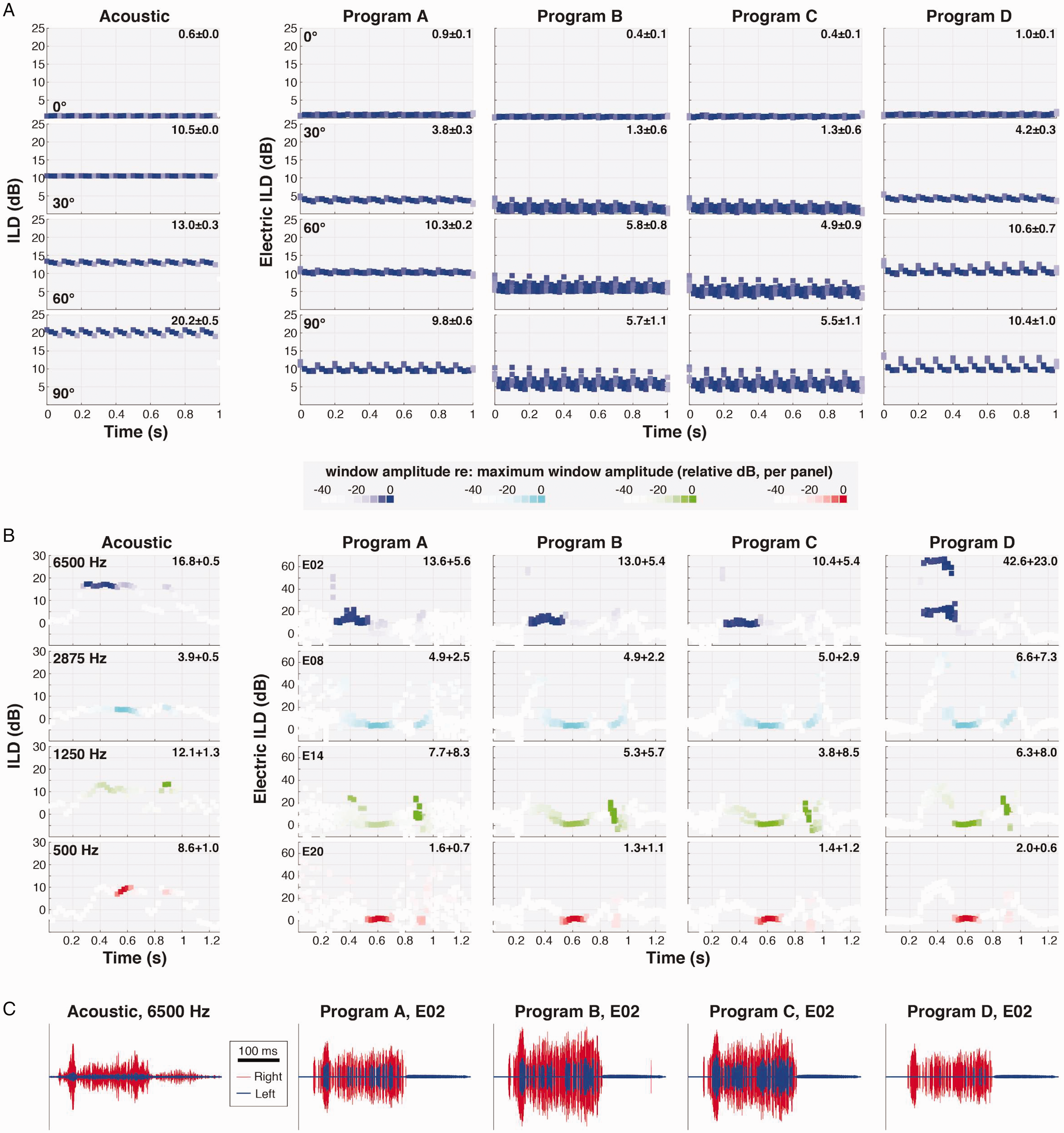
Temporal Variation of ILDs Across BiCI Programs. A: Panels illustrate ILD cues computed within a 50-ms running temporal window for a 10-Hz SAM tone, 4375-Hz carrier frequency, at four different azimuths (as labeled). The color intensity of each point is scaled according to the average binaural level (RMS amplitude) of the signal within the corresponding temporal window. Acoustic ILDs are illustrated in the left column; electric ILDs on electrode E05 for four different CI program configurations (see “Materials and Methods” section) are given in the rightward columns. CI stimuli were presented at 45 dBA, near the middle of the programmed dynamic range; acoustic stimuli were presented at 65 dBA, which provided the best SNR for acoustic analyses. Numbers in the upper right of each panel give the weighted mean and SD of ILD (or electric ILD) across temporal windows (see text). B: ILDs as in A, but for the speech token “seek” within four different frequency bands (center frequencies as labeled) with the source at 30˚ azimuth. C: Representative brief acoustic and CI signal segments used in the calculations in B (here for the 6500 Hz channel/E02), illustrating sporadic pulse allocations in the left electrode that led to large fluctuations in electric ILDs (see text). ILD = interaural level difference.

Figure 8B plots time-varying ILD calculations for the word “seek” within four electrode channels at a fixed azimuth (+30°). Compared with acoustic data, for which ILD fluctuation was again minimal for temporal windows conveying the majority of signal energy, all BiCI-transmitted ILDs (Programs A–D) fluctuated substantially, illustrating the challenge posed by an ecological signal that is both temporally and spectrally dynamic. Although mean ILD values were again generally slightly reduced with ADRO enabled (Programs B and C), the most striking feature of BiCI ILDs was extreme fluctuation over brief signal segments, particularly in the higher frequency channels. The apparent source of such fluctuation is illustrated in Figure 8C, which plots acoustic and BiCI signal segments for the 6500 Hz channel during the initial / s / (note 100-ms scale bar) for a single repetition of “seek.” Whereas a prominent head-shadow effect led to uniform attenuation of the acoustic signal at the left ear (left column, blue signal), the same head shadow led to epochs with no BiCI pulses in the left electrode (E02). During selected 50-ms epochs, the left electrode transmitted only a few pulses while the right electrode transmitted several dozen; pulse allocations were more balanced across other epochs, with the result that the ILD could fluctuate tens of decibels window-to-window (Figure 8B, top row). We note that this result is effectively the ILD-manifestation of time-varying symmetry as quantified in Figure 3. The magnitude of fluctuation for the specific instance highlighted in Figure 8C (E02, / s / in “seek”) appeared slightly reduced for the Programs B and C that included ADRO, but large ILD fluctuations were evident on one or more electrodes for all programs.

General Discussion

Overview

The purpose of this report was to quantify the transmission of binaural cues (ITDs and ILDs) by BiCI sound processors implementing a coding strategy in wide clinical use. It has long been suggested that bilaterally independent processing could lead to distortions of binaural cues (particularly ITD)—and that such distortions could partially explain the relatively poor binaural and spatial hearing outcomes in BiCI users, as well as listeners’ reliance on ILDs over ITDs (see “Introduction” section). Here, we consider the perceptual implications of the cue measurements reported and limitations of this study.

Impacts of Asymmetric Spectral Peak-Picking

All measurements were completed using ACE, a clinically widespread n-of-m spectral peak-picking strategy (∼97% of Cochlear device users, S. Steele, personal communication, December 4, 2020). The spectral peak-picking process was independent in each processor, resulting in an independent allocation of pulses across each electrode array. Independent allocation often caused asymmetric pulse counts between the left and right channels. Symmetry was typically high for near-midline sources but declined at large azimuths (see Figure 3E). However, particularly for electrode pairs receiving low-to-intermediate pulse allocations, poor symmetry could be observed at any azimuth (see Figure 6A). Poor symmetry was found to be disruptive to binaural cues, with poorer symmetry resulting in higher cue variability (see Figure 6B and C). In the BBN condition for some electrodes, the independent peak-picking process also created spurious leftward ILDs despite rightward source azimuths (sometimes infinite leftward ILDs; see Figures 3 and 4; cf. Archer-Boyd & Carlyon, 2019; Dorman et al., 2014; Kelvasa & Dietz, 2015). To ensure integrity of transmitted ITD and (to a lesser extent) ILD cues, the selection of active electrodes in a given processing period would likely need to be linked (see later). Non-peak-picking strategies, such as CIS, would not be subject to this requirement but were not evaluated in this study.

To our knowledge, there is currently no empirical perceptual comparison of static sound-source localization for linked versus independent spectral peak-picking strategies. However, a small body of perceptual research on other tasks does exist. Linked spectral peak-picking did not significantly affect auditory motion discrimination, although some participants showed benefit (Dennison et al., 2019). In addition, some research suggests that linked spectral peak-picking improves speech understanding in spatially separated noise (Gajecki & Nogueira, 2020). A modeling study suggested that independent spectral peak-picking would negatively affect BiCI localization (Kelvasa & Dietz, 2015), and that independent processing could under some conditions cause stronger stimulation on contralateral electrodes and therefore create opposite-signed ILDs. This prediction was later borne out in BiCI electrode recordings (Kan et al., 2018) and was observed in this study across multiple stimuli and presentation levels. Further research is needed to assess the perceptual importance of such binaural cue distortions associated with linked and independent n-of-m processing strategies—and prospective benefit of mitigating such distortions.

Impact of Level Saturation and Unlinked Compression on Transmitted ILDs

Presentation level affected binaural cues independent of its influence on pulse-count asymmetry (which was worst at low presentation levels, Figure 3). Most prominently, as presentation level increased, ILDs systematically decreased for all electrodes. Level compression in CI outputs (due to both nonlinear acoustic level-to-current mapping and AGC) has been predicted (Kan & Litovsky, 2015; Kelvasa & Dietz, 2015; Majdak et al., 2011) and observed (Kerber & Seeber, 2012) to constrain the range of transmitted ILDs. Effective limiting of ILDs, which is expected to be more severe at high presentation levels (due to saturation as the upper level of the acoustic dynamic range is reached), was evident in the present data both at the whole-waveform level and on a time-varying basis (cf. Archer-Boyd & Carlyon, 2019). At lower presentation levels (e.g., 45 dBA, Figure 8), particularly for spectrotemporally dynamic stimuli (Figure 8B), very large fluctuations in ILD (tens of decibels in variation over time within a 50-ms running temporal window) were observed—a combinatorial effect of compression and time-varying symmetry in pulse allocations. Targeted measurements without interference from independent spectral peak-picking will be required to further evaluate distortions attributable to specific preprocessing algorithms.

Further perceptual measurements are required to elucidate the practical impacts of BiCI ILD compression and time-variance. Compressed ILDs have been shown to result in poor localization accuracy (Dorman et al., 2014). As the natural variation of ILD cues across azimuth and ILD magnitude-dependent variation in the precision of ILD perception both appear to affect localization performance (see Brown et al., 2018), joint measurements of BiCI perceptual ILD acuity and actual ILDs transmitted by clinical processors across azimuth may be especially informative in interpreting “real-world” BiCI localization performance. Regarding time-varying ILD fluctuation, existing studies indicate that sufficiently slow ILD changes (of a few Hz or less) may be perceived as lateral movement of a sound source (e.g., Blauert, 1972; Grantham, 1984). Fluctuations were observed on multiple time scales in the present recordings; further perceptual measurements will be important to establish under what circumstances dynamic BiCI ILDs are perceived as source movement, increased “image width,” or both (cf. Archer-Boyd & Carlyon, 2019). Directly relating the measured electric ILDs of the present report to ILD sensitivity reported in the literature, which has often been measured via controlled single-electrode direct stimulation (e.g., Litovsky et al., 2010; van Hoesel & Tyler, 2003) is tenuous. Our measurements were affected by two factors that exert a strong overall level dependence—the nonlinear conversion of level to current, and AGCs, which were also unlinked between the ears. Nonetheless, order-of-magnitude variation in electric ILDs across time despite a static source, and electric ILDs that cease to vary with changes in azimuth at high sound levels, could reasonably be expected to impact perception; further study is indicated.

Transmission of ITD via Independent Processor Clocks

Previous literature has shown that envelope ITD cues measured from BiCI electrodes can deviate from expected acoustic values (e.g., Kan et al., 2018) and exhibit high variability (e.g., Rodriguez & Goupell, 2015). Similar data were measured here, such as inflated envelope ITDs in some channels (see Figures 4C and 5) and wide variability in the ITD cues transmitted across electrodes (see Figure 6). However, an oft-suggested culprit for poor BiCI ITD sensitivity—temporally independent processors—was not found to be a primary constraint on the transmission of envelope ITD. This observation extended across ecological stimuli (speech) and multiple preprocessing programs (data not shown). Pulse-timing ITD was found to vary over time, even at 0° azimuth, due to unsynchronized processors (Figure 7A), and arbitrarily restarting one of the processors created a new and arbitrary pulse-timing ITD (Figure 7B and C, left panels). However, these variations in pulse-timing ITD did not systematically affect envelope ITDs (Figure 7B and C, right panels). These data thus suggest that unsynchronized BiCI clinical processors can convey useful envelope ITD information, provided that both devices are conveying a similar number of pulses (pulse-count symmetry), and that pulse rate is sufficiently high to prevent a listener from perceiving pulse ITD (Laback et al., 2015). That is, it appears that linking of the channel selection process, as opposed to the processor clocks, is most important for transmission of informative envelope ITDs in an n-of-m strategy. Notably, failures in symmetry (asymmetric pulse allocation, even if only temporarily) can occur in the vicinity of prominent envelope fluctuations such as transient rises/falls, disrupting the ITDs transmitted by these brief but potentially salient signal segments.

Whereas comparisons between measured BiCI ILDs and ILD perception are complicated by differences in units of amplitude, comparisons are somewhat more straightforward for ITD measurements, which depend on the same (µs) unit system. Under controlled conditions using computer-linked bilaterally synchronized direct stimulation—which avoids disruptions from asymmetric pulse allocations or processor clock disparities—envelope ITD thresholds at single-electrode pairs for ∼1,000 pps pulse trains can be on the order of ∼100 µs or slightly better (e.g., Noel & Eddington, 2013), approaching NH thresholds for analogous acoustic stimuli (L. R. Bernstein & Trahiotis, 2002). Suprathreshold envelope ITDs also elicit similar lateralization responses in BiCI and NH listeners, particularly after accounting for subject age (Anderson et al., 2019). In less-controlled multi-electrode presentation using clinical processors, envelope ITD thresholds can range from hundreds of microseconds in some subjects to unmeasurable in others (Grantham et al., 2008; Kerber & Seeber, 2013; Laback et al., 2004). While the present data suggest that envelope ITDs on the order of several hundred microseconds (associated with lateral source azimuths) can be conveyed via ACE, data also demonstrate intrinsic ITD variability commonly exceeding 100 µs and approaching 1,000 µs in some cases. There are few data on the ITD sensitivity of subjects wearing BiCI processors using ACE, but one conference report indicated than some listeners can detect ITDs on the order of a few hundred microseconds (Kan et al., 2017; cf. Kerber & Seeber, 2013). Further measurements of clinical processor-mediated ITD sensitivity—particularly contrasting stimulation strategies that control or do not control ITD variability—could prove informative.

Limitations and Future Directions

Comparison of acoustic and BiCI ILDs is complicated by multiple factors. As discussed in the foregoing sections, BiCI ILDs effectively represent differences in current level outputs, while acoustic ILDs are differences in the sound pressure levels of signals at the two ears. An additional consideration is that behind-the-ear microphones (like those on the CI sound processors) and in-the-ear microphones (like those on the manikin) do not receive the same ILDs to begin with; behind-the-ear microphones receive smaller and less monotonic ILDs, and their nonmonotonicities manifest at different azimuths (see Figure 4A; Mayo & Goupell, 2020). Nonetheless, useful comparisons within BiCI conditions are readily made, and qualitative comparison of electric and acoustic ILDs (e.g., the presence or absence of “negative” values) can still prove informative.

In the present data set, detailed assessments of the “binaural” effects of various processing programs and nonlinear level mapping across channels were partially confounded by low pulse-count symmetry, apparently an inherent limitation of bilaterally independent spectral peak-picking. It would be desirable to complete a parallel set of measurements using a stimulation strategy that preserved symmetry to enable further evaluation of other processing/program features of interest. A non-peak-picking stimulation strategy such as CIS could serve this purpose, as could an experimentally linked peak-picking strategy (cf. Gajecki & Nogueira, 2020). Some evidence suggests that the different stimulation strategies implemented across CI manufacturers and devices may afford listeners varying localization performance (Killan et al., 2019), a result that could be further informed by future empirical recordings from a variety of devices.

Finally, all reported measurements were taken in a “simple” listening situation with a single, stationary source and no background noise, reverberation, or other sources of interference. While these data may thus serve as a reference for behavioral measurements completed in similarly simple acoustic settings, understanding device-related constraints on behavioral outcomes in real listening contexts will benefit from future measurements using more complex stimuli.