Sage Journals: Discover world-class research

Abstract

Bilateral cochlear-implant (BiCI) users are less accurate at localizing free-field (FF) sound sources than normal-hearing (NH) listeners. This performance gap is not well understood but is likely due to a combination of compromises in acoustic signal representation by the two independent speech processors and neural degradation of auditory pathways associated with a patient’s hearing loss. To exclusively investigate the effect of CI speech encoding on horizontal-plane sound localization, the present study measured sound localization performance in NH subjects listening to vocoder processed and nonvocoded virtual acoustic space (VAS) stimuli. Various aspects of BiCI stimulation such as independently functioning devices, variable across-ear channel selection, and pulsatile stimulation were simulated using uncorrelated noise (N_u), correlated noise (N₀), or Gaussian-enveloped tone (GET) carriers during vocoder processing. Additionally, FF sound localization in BiCI users was measured in the same testing environment for comparison. Distinct response patterns across azimuthal locations were evident for both listener groups and were analyzed using a multilevel regression analysis. Simulated implant speech encoding, regardless of carrier, was detrimental to NH localization and the GET vocoder best simulated BiCI FF performance in NH listeners. Overall, the detrimental effect of vocoder processing on NH performance suggests that sound localization deficits may persist even for BiCI patients who have minimal neural degradation associated with their hearing loss and indicates that CI speech encoding plays a significant role in the sound localization deficits experienced by BiCI users.

Keywords

bilateral cochlear implant sound localization vocoder

Introduction

Cochlear implants (CIs) are used at increasing rates to provide hearing to individuals with severe-to-profound hearing loss. Many patients receive bilateral cochlear implants (BiCIs) in an effort to improve spatial hearing abilities, such as sound localization and speech understanding in noisy environments, relative to the single-CI listening mode. Numerous free-field (FF) studies have established that compared with unilateral CI use, bilateral CIs improve sound localization accuracy along the horizontal plane (Grantham, Ashmead, Ricketts, Labadie, & Haynes, 2007; Litovsky, Parkinson, & Arcaroli, 2009; Majdak, Goupell, & Laback, 2011; Nopp, Schleich, & D’Haese, 2004; Seeber, Baumann, & Fastl, 2004; Van Hoesel, 2004; Seeber & Fastl, 2008). For example, Litovsky et al. (2009) reported that root mean square (RMS) errors along the horizontal plane for 17 postlingually deafened adult BiCI users were overall 30° lower for bilateral implant use compared with unilateral use. Other studies have also shown similar effect sizes. Despite the added benefit of having two implants, BiCI users still demonstrate large deficits in spatial hearing performance compared with normal-hearing (NH) listeners (Grantham et al., 2007; Litovsky, 2011; Litovsky et al., 2012). For example, Grantham et al. (2007) reported that overall errors for adult BiCI users were on average 29° compared with the 7.6° observed for NH listeners, demonstrating that bilateral stimulation alone does not restore sound localization abilities.

Such a gap in localization performance could arise from a number of fundamental differences between NH listeners and BiCI users; however, investigating possible sources for these localization deficits has been complicated by the variability in performance across BiCI patients due to numerous factors. Variable periods of auditory deprivation can result in differing amounts of neural degeneration (Coco et al., 2007; Leake, Hradek, & Snyder, 1999), and human temporal bones studies have demonstrated that the extent of auditory nerve survival can vary significantly among cochleae (Hinojosa & Marion, 1983; Nadol, Young, & Glynn, 1989; Otte, Schunknecht, & Kerr, 1978). For BiCI patients, such issues are further complicated by the likelihood of asymmetrical neural degeneration between the two ears, as many patients may undergo hearing loss at different rates between the two ears. Despite extensive research on horizontal-plane sound localization in BiCI users, little is known about the relative contributions of degraded neural circuitry.

Another important factor is the manner in which acoustic signals are encoded and presented to the implanted patient’s auditory system. The work presented here focuses on exploring possible ways in which degraded auditory signal representation may account for differences in performance between NH listeners and BiCI users. It is generally thought that certain acoustical cues necessary for sound localization are not adequately provided to BiCI users. For example, asymmetries in microphone characteristics (Van Hoesel, Ramsden, & Odriscoll, 2002), variable electrode insertion depths (Kan, Stoelb, Litovsky, & Goupell, 2013), uncoordinated stimulation between the bilateral devices (Laback, Pok, Baumgartner, Deutsch, & Schmid, 2004; Seeber et al., 2004; Seeber & Fastl, 2008), and spread of electrical current across adjacent electrodes (Fu & Nogaki, 2005; Landsberger, Padilla, & Srinivasan, 2012; Van Hoesel & Tyler, 2003) could all affect acoustical cue presentation to the auditory system. In NH listeners, sound localization along the horizontal plane requires the binaural processing of acoustical cues. These cues include interaural time differences (ITD) in the acoustic temporal fine structure (TFS) of low frequencies (<1.5 kHz), interaural level difference (ILD) at high frequencies, and ITDs in the slowly varying amplitude modulations of the acoustic envelopes (ENVs). In general, ITDs in the low-frequency TFS have been shown to be the dominant cue (Blauert, 1997; Macpherson & Middlebrooks, 2002; Middlebrooks & Green, 1991; Wightman & Kistler, 1989).

Previous FF studies in BiCI users have demonstrated that these listeners predominantly use ILDs with limited use of ITD information (Laback, Pok, et al., 2004; Litovsky et al., 2009, Litovsky, Jones, Agrawal, & van Hoesel, 2010; Seeber & Fastl, 2008; Van Hoesel, 2008). These results are not surprising because CI signal processing discards acoustic TFS and encodes the acoustic ENVs. However, studies using research processors that bypass the clinical CI speech processors and deliver tightly controlled binaural cues via coordinated stimulation have shown that many BiCI users exhibit sensitivity to ILDs, as well as ITDs presented at low pulse rates (Litovsky et al., 2010, 2012; Van Hoesel, 2007; Van Hoesel, Jones, & Litovsky, 2009). It is noteworthy that ITD sensitivity in BiCI users is generally worse than that seen in NH listeners (see Litovsky et al., 2010, 2012). Many BiCI users also exhibit sensitivity to ITDs contained in the ENVs of high-rate stimuli that are amplitude modulated at low rates (Laback, Pok, et al., 2004; Seeber & Fastl, 2008; Van Hoesel & Tyler, 2003; Van Hoesel et al., 2009), and sensitivity is often comparable to that seen with ITDs in low-rate stimuli (Majdak, Laback, & Baumgartner, 2006; Van Hoesel, 2007; Van Hoesel et al., 2009). For modulated signals such as speech, ITDs extracted from the ENVs of the high-rate stimulation could be potentially useful for BiCI sound localization (Loizou, 1999; Wilson & Dorman, 2008). The aforementioned studies have identified similarities between BiCI and NH listeners, as well as gaps in performance under ideal conditions in which binaural cues are presented with precision. However, in a clinical setting when patients listen in the FF with their processors, the technical features listed earlier are not taken into consideration.

Simulations using vocoders can be powerful in that some effects of CI processing can be evaluated in the healthy auditory system of NH listeners while bypassing subject-dependent factors associated with hearing loss and cochlear implantation (Dorman, Loizou, Fitzke, & Tu, 1998; Dorman, Loizou, & Rainey, 1997; Goupell, Majdak, & Laback, 2010; Qin & Oxenham, 2003; Shannon, Zeng, Kamath, Wygonski, & Ekelid, 1995; Wilson et al., 1991). Another advantage of using vocoders with NH listeners is the reduced across-subject variability, in contrast to the ubiquitous high variability in CI users. Vocoders simulate CI speech encoding by processing acoustic signals in a similar manner as clinical speech processors. Present day CI speech encoding strategies filter incoming acoustic signals into a small number of discrete frequency bands (typically 12–22 channels between 150 Hz and 8 kHz) corresponding to the number of electrode contacts used by the particular device. The acoustic ENV within each channel is extracted and transmitted via high-rate electrical pulse stimulation on electrode contacts spaced along the tonotopically organized cochlea, while the TFS of the signal is discarded (Loizou, 1999). In traditional vocoders, the ENVs of the acoustic signals extracted from the frequency bands can be used to modulate narrowband noise or sine tone carriers, to stimulate specific places along the cochlea. Recently, Gaussian-enveloped tone (GET) carriers have also been used to simulate CI sound processing (Goupell et al., 2010; Goupell, Stoelb, Kan, & Litovsky, 2013).

In GET vocoders, a Gaussian-shaped temporal envelope modulates a sine tone to generate a brief acoustic pulse that is replicated and delayed to create a pulse train. As GET pulses excite a larger frequency spectrum compared with a sine tone (van Schijndel, Houtgast, & Festen, 1999), the GET vocoder simulates in some ways the spread of electrical current along the basilar membrane, in addition to presenting pulsatile stimulation. Noise (Bingabr, Espinoza-Varas, & Loizou, 2008; Fu and Nogaki, 2005) and sine (Crew, Galvin, & Fu, 2012) vocoders can also simulate current spread and have been commonly used to probe acoustic features necessary for speech reception in various listening environments (Dorman & Loizou, 1997; Dorman, Loizou, & Fitzke, 1998; Qin & Oxenham, 2003); however, the GET vocoder has been argued to better simulate the electrical stimulation in clinical CI devices (Goupell et al., 2010, 2013). A recent study comparing lateralization of ITDs and ILDs showed that NH subjects listening to GET pulse trains performed similarly to BiCI subjects (Kan et al., 2013). Additionally, Goupell et al. (2010) used GET vocoders to process VAS stimuli and showed that localization performance along the median plane in NH listeners deteriorated with decreased number of channels. Results using the GET stimulation also suggested that current CI encoding strategies should have a sufficient number of channels for vertical-plane sound localization capabilities. To date, the effect of CI speech encoding on sound localization abilities along the horizontal plane in NH listeners has not been previously tested.

The present study created a realistic BiCI simulation in NH listeners by combining virtual acoustic space (VAS) and vocoder techniques, and then directly compared this NH performance with that tested in BiCI users in the same FF testing environment. We measured head-related transfer functions (HRTFs) for each NH subject, and individualized VAS speech stimuli were created for localization testing to ensure comparable localization performance in the control condition. Each subject’s VAS stimuli were then processed using either a noise or GET vocoder, and localization performance was measured. The baseline data from this work have the potential to lead to investigations of the numerous additional factors that might affect BiCI sound localization, such as electrode mismatch and spread of current (see Fu & Nogaki, 2005; Kan et al., 2013) while circumventing the confounding variable degrees of neural degradation associated with BiCI users.

Methods

Participants

Twenty subjects participated in this study. Ten NH subjects had audiometric pure-tone thresholds below 15 dB HL for octave frequencies spanning 250–8000 Hz with no asymmetry in hearing thresholds exceeding 10 dB at any of the frequencies tested and were native speakers of American English. Subjects were either students or staff at the University of Wisconsin-Madison and were paid for their participation. Ten postlingually deafened BiCI users with CI24 and CI512 family of implants, and who used Freedom or N5 speech processors (Cochlear Ltd., Sydney, Australia), participated in this study. All subjects had a minimum of 1 year of bilateral implant experience. BiCI subjects traveled to the University of Wisconsin-Madison for testing and received payment, per diem, and were reimbursed for all travel-related costs. The profile and etiology of the BiCI users are shown in Table 1. All experimental procedures followed the regulations set by the National Institutes of Health and were approved by the University of Wisconsin’s Human Subjects Institutional Review Board. The BiCI subjects were tested only on FF sound localization to compare their performance with that of the NH subjects listening to vocoded stimuli. Thus, no HRTF measurements were made for the BiCI users, and they were not tested with any VAS or vocoded stimuli.

Table 1.

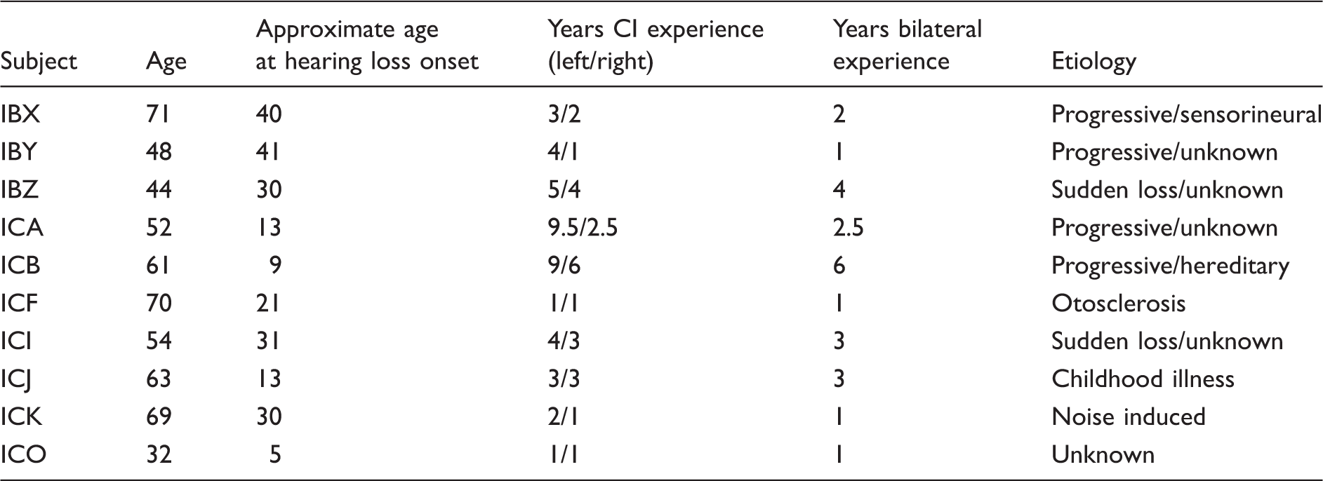
Profile and Etiology of BiCI Subjects.

Subject	Age	Approximate age at hearing loss onset	Years CI experience (left/right)	Years bilateral experience	Etiology
IBX	71	40	3/2	2	Progressive/sensorineural
IBY	48	41	4/1	1	Progressive/unknown
IBZ	44	30	5/4	4	Sudden loss/unknown
ICA	52	13	9.5/2.5	2.5	Progressive/unknown
ICB	61	9	9/6	6	Progressive/hereditary
ICF	70	21	1/1	1	Otosclerosis
ICI	54	31	4/3	3	Sudden loss/unknown
ICJ	63	13	3/3	3	Childhood illness
ICK	69	30	2/1	1	Noise induced
ICO	32	5	1/1	1	Unknown

Equipment

Measurement of HRTFs and behavioral sound localization testing were conducted in the same sound booth. The booth had internal dimensions of 2.90 × 2.74 × 2.44 m (IAC, RS 254 S), and additional sound-absorbing foam was attached to the inside walls to reduce reflections. A Tucker-Davis Technologies (TDT) System 3 was used to select and drive an array of 19 loudspeakers (Cambridge SoundWorks) arranged on a semicircular arc of 1.2 m radius. Loudspeakers were positioned in 10° increments along the horizontal plane between ± 90° and were hidden behind a dark, acoustically transparent curtain. Subjects sat in the center of the array with their ears at the same height as the loudspeakers. For FF localization testing, stimuli were calibrated to output at 60-dB sound pressure level (SPL) using a digital precision sound level meter (System 824, Larson Davis; Depew, NY) placed at the center of the arc where the subject’s head would be positioned. The VAS stimuli were presented via in-ear headphones (ER-2, Etyomtic Research) using the TDT System 3 with a 48-kHz sampling rate and were calibrated so that the perceived output level of the headphones matched that of the FF presentations. Headphone calibrations were made using the sound level meter and an artificial ear coupler (2-cc coupler, G.R.A.S.; Larson Davis, Depew, New York). All stimulus presentations and data acquisition were done using custom MATLAB software (Mathworks, Inc., Natick, MA). All analyses were carried out using R software version 3.0.2.

HRTF Measurements

For each NH subject, individual HRTF measurements were made for the 19 loudspeaker locations, using a blocked-ear technique (Møller, 1992). Subjects were asked to face the front (i.e., speaker position 0°) and to remain stationary during each stimulus presentation. Golay codes (200 ms long, five repetitions) were used as probe signals for HRTF recordings, and the in-ear responses were recorded by a blocked-meatus microphone pair (HeadZap binaural microphones, AuSim, Mountain View, CA) placed in the entrance of each ear canal. Microphone output signals were amplified (MP-1, Sound Devices) and recorded using a TDT RP2.1 at 48 kHz. Traditionally, HRTFs are defined with reference to the sound pressure in the middle of the head with the listener absent (Møller, 1992). To obtain an HRTF for a particular source location, the microphone recordings at the ears can be divided by the response measured with only the microphone at the location in the center of the loudspeaker array. This effectively removes the loudspeaker frequency characteristics in HRTFs. However, in this experiment, the loudspeaker characteristics were not removed from the digital filters used to synthesize the VAS stimuli because we were interested in preserving these characteristics for a direct comparison of FF localization performance to headphone presentations. Thus, the loudspeaker frequency characteristics were not removed from the HRTFs.

It should also be noted that the HRTF recording procedures used in the current study may not be representative of the BiCI condition for most patients, as the majority of CI processors use microphones that are placed behind the ear. However, the aim of the present study was to exclusively investigate the effect of CI speech encoding on NH sound localization. As such, the HRTF measurements made with microphones placed in the ears ensured that individual-specific acoustical cues for each subject were intact prior to vocoder processing. Additionally, the acoustical cues captured by microphones in the ear should be natural for NH listeners, so no adaptation to these cues or training was required for the VAS stimuli.

Stimuli

Nonvocoded stimuli

NH listeners were tested with stimuli consisting of 10 monosyllabic consonant-nucleus-consonant (CNC) words spoken by a male talker. Each speech token (beam, cape, car, choose, chore, ditch, dodge, goose, knife, and merge) was filtered by the HRTF measurements to create VAS stimuli for each spatial location. These stimuli provided a control condition for comparison to performance measured with the vocoded stimuli. To make comparisons of sound localization performance between nonvocoded and vocoded stimuli, test stimuli were low-pass filtered to match the bandwidth of the vocoder. A fourth-order Butterworth filter with an 8-kHz cutoff frequency was applied to the original speech stimuli prior to HRTF-filtering for VAS presentation. Subjects confirmed that the perceived loudness of the VAS stimuli presented through the headphones matched the loudness of FF stimuli presented from the loudspeaker array. For the BiCI listeners, FF sound localization performance was measured using four bursts of pink noise each with a 10-ms rise–fall time and 170 ms in duration. These stimuli and parameters were chosen to optimize the FF localization performance in the BiCI listeners (Litovsky et al., 2009; Van Hoesel & Tyler, 2003).

Vocoded stimuli

Vocoded stimuli were generated by processing the VAS stimuli through an eight-channel vocoder, spanning a range of 150 to 8000 Hz. The stimuli were band-pass filtered using fourth-order Butterworth analysis filters with evenly spaced center frequencies as calculated using the Greenwood function (Greenwood, 1990). The center and corner frequencies of the analysis filters used in the vocoders are shown in Table 2. Signals were then half-wave rectified and low-pass filtered at 50 Hz by a second-order Butterworth filter for envelope extraction and sideband removal. The envelopes of each band were then used to modulate one of three different acoustic carriers (identified by the subscript): uncorrelated noise (_Nu), correlated noise (_N0), or Gaussian-enveloped tones (_GET). The modulated carriers for each frequency band were then summed together separately for left and right channels to create the final stimuli.

Table 2.

Frequency Allocation for the Vocoder Channels Used in This Study.

Channel	Frequency (Hz)
Channel	Lower	Upper	Center (noise vocoder)	Center (GET vocoder)
1	150	301	213	218
2	301	531	401	405
3	531	879	684	688
4	879	1406	1120	1160
5	1406	2203	1760	1763
6	2203	3409	2741	2744
7	3409	5235	4223	4228
8	5235	8000	6472	6475

The carriers used in this experiment were chosen to simulate different aspects of cochlear implant stimulation. The NH_N0 and NH_Nu stimuli were intended to simulate the presence and absence of coordinated binaural stimulation, respectively, while preserving level and envelope cues imposed by the HRTF filtering of the stimuli. Wideband noise carriers were generated independently for each channel, and prior to envelope modulation, were band-pass filtered with the same analysis filters described earlier. For the NH_N0 stimuli, the same noise carrier was used for both ears. For the NH_Nu stimuli, different noise carriers were used for each ear. The NH_GET pulse trains were used to simulate CI electrical stimulation. A 100-Hz GET pulse train centered at each of the center frequencies in Table 2 was generated in a manner similar to that described in Goupell et al., (2010), where the bandwidth of the Gaussian pulse was equal to the bandwidth of the corresponding band-pass filter. The left and right signal envelopes were used to modulate the GET pulse train. It should be noted that the same GET pulse train was used to carry the left and right signal envelopes, which means the timing of the envelope and TFS of the GET pulses were synchronized between the left and right ears before modulation with the speech envelope. Hence, the left and right ear signals varied only by the envelope cues extracted from the VAS stimuli.

Testing Procedure

Listeners sat on a chair in the center of the loudspeaker array and were asked to remain still with their gaze fixated on a visual marker at 0° during all stimulus presentations. Localization stimuli were presented from either the loudspeaker array (FF) or through headphones (VAS and vocoded conditions) at 60 dB SPL. Additionally, ± 4 dB level roving was applied to the stimuli prior to presentation to minimize the use of monaural level cues. Spectral roving was also applied to the pink noise stimuli by dividing the energy spectrum of stimulus into 50 critical bands and assigning a random intensity ( ± 10 dB) to each band (Wightman & Kistler, 1989). Listeners were aware of the azimuthal range of loudspeakers (−90° to 90°) and that sounds were presented only from frontal source locations within this range; however, the loudspeakers remained hidden behind an acoustically transparent curtain. Each condition was presented twice as a separate block of 95 trials (5 stimulus presentations × 19 locations), each typically lasting ∼20 min. The CNC words were randomly presented once from each of the target locations. Sound localization testing was conducted in three 2-hr sessions.

Trials were self-initiated by pressing a button on a touch screen monitor placed in front of the subject and positioned such that it had a minimal effect on the acoustic stimuli. Following stimulus presentation, a graphical user interface (GUI) with an image of an arc representing the arc of loudspeakers was displayed on the touch screen monitor. Subjects indicated their response by placing a digital marker anywhere on the arc image corresponding to the perceived sound source location. To facilitate perceptual correspondence between the spatial locations in the room and the arc image on the touch screen, visual markers were placed at 45° increments both along the curtain in the room and on the GUI.

Results

For comparisons with previous BiCI FF studies, sound localization performance was evaluated by computing the overall RMS error for all 190 trials per condition. Assuming a uniform distribution of random responses (i.e., guessing), chance performance was calculated to be 75.6° within the full range of responses and 39.7° for responses that were within the correct left or right hemisphere. The VAS techniques employed here were validated by comparing NH_FF and NH_VAS performance. The average RMS error was slightly smaller for the FF condition than the VAS condition (NH_FF: 8.2 ± 1.9°; NH_VAS: 11.2 ± 1.7°); this is consistent with previous findings that localization of FF sounds is generally better than for virtual sounds (Middlebrooks, 1999). Additionally, the average RMS error for the NH_VAS condition here was comparable to the average lateral RMS error (12.4 ± 2.2°) recently reported for NH subjects listening to VAS stimuli (Majdak et al., 2011). These findings indicate that the VAS techniques reported here provided an adequate representation of FF stimulus presentation.

Figure 1 shows the across-subject average RMS error (bar, mean) and standard deviation (error bars, ± SD) for NH subjects in the four conditions tested as well as the BiCI subjects. There was a clear increase in the average RMS error between the NH_VAS (11.2 ± 1.7°) and the three vocoded conditions, NH_Nu (36.4 ± 6.0°), NH_N0 (40.6 ± 11.0°), and NH_GET (34.2 ± 7.7°). A one-way, repeated-measures analysis of variance (ANOVA) of the RMS errors measured for the NH subjects on the four listening conditions showed a significant main effect, F(3, 9) = 89.62, p < .001. Scheffe’s post hoc analyses revealed significant differences between the VAS and all the vocoder conditions (p < .05), indicating that vocoder processing of VAS stimuli significantly increased localization errors. However, there were no significant differences between the three vocoder conditions. For BiCI subjects, the average RMS error, BiCI_FF (27.9 ± 12.3°), was consistent with previously reported data (Grantham et al., 2007; Litovsky et al., 2009). Independent samples t tests were conducted to test for differences in RMS errors between each of the NH conditions and the BiCI_FF data. Pairwise test with Bonferroni correction revealed that the RMS errors in the BiCI_FF condition were significantly larger than the NH_VAS condition, t(18) = −10.693, p < .001. Additionally, the NH_Nu and NH_N0 conditions had significantly larger RMS errors than the BiCI_FF condition—NH_Nu: t(18) = 3.561, p = .002; NH_N0: t(18) = 3.378, p = .003. The comparison between BiCI_FF and NH_GET approached significance but was non-significant following the p-value adjustments for multiple comparisons, t(18) = 2.232, p = .039. Thus, the BiCI subjects performed worse than the NH listeners listening to VAS stimuli. However, BiCI subjects generally outperformed NH listeners, following vocoder processing of the VAS stimuli.

Figure 1.

Summary of localization performance. The average RMS error (bars, mean) and standard deviation (error bars, ±SD) for NH and BiCI subjects are plotted. The asterisk indicates statistically significant results for comparison of the average RMS across subjects for each listening condition and post hoc analysis (see text for details).

Although the group analysis revealed no difference in RMS errors between the vocoder conditions, we wanted to explore whether differences in response distributions and localization error patterns across target locations existed. For this analysis, localization errors were calculated as the absolute difference between target and response angles. The absolute error measure better represents localization accuracy, that is, the systematic error as measured by the bias, whereas the RMS error measure better represents localization precision, that is, the error variability across all locations (Majdak et al., 2011). The average absolute errors for the NH subjects were VAS (9.4 ± 2.3°), VC_Nu (28.4 ± 4.6°), VC_N0 (31.3 ± 8.2°), and VC_GET (27.0 ± 6.4°). For BiCI subjects, the average absolute error (21.4 ± 3.6°) was consistent with the absolute lateral error (19.3 ± 2.3°) recently reported for BiCI users listening to VAS stimuli (Majdak et al., 2011). To observe target location effects, the average absolute error (bar, mean) and standard error (error bars, ± SE) as a function of target angle is plotted in Figure 2(a) for each condition. Additionally, subject responses were binned into 10° increments, and counts were average across subjects for each target location (Figure 2(b), mean and ± SE). Varying patterns in the average RMS errors and response distributions across target locations were observed for the different listening condition. For example, the VC_N0 condition on average resulted in small RMS errors at target location 0° and large errors for target locations ± 90° (Figure 2(a), VC_N0 panel). However, the lower RMS errors seem to be a result of more target sounds being heard from the front locations (Figure 2(b), VC_N0 panel). Given that distinct patterns were observed for the different vocoder conditions, we wanted to investigate whether any of the vocoders produced a similar localization error pattern as those measured in the BiCI users.

Figure 2.

Absolute localization error and response distribution across target angles. (a) The across-subject average absolute difference between target and response angles (bars, mean) and standard deviation (error bars, ± SD) for each target location. (b) The average binned responses for each target angle across subjects, with responses placed in the nearest 10 bin.

To compare localization performance patterns between NH and BiCI listeners, a multilevel regression analysis (Mirman, 2014) was used to model and analyze the data. The pattern of errors (Figure 2(a)) and distribution of responses (Figure 2(b)) across target locations for each condition exhibited a rough symmetry moving from the central to lateral target locations on either side. Due to this observation, the absolute localization errors were collapsed as a function of target deviance from the center speaker (0°), that is, the absolute target angle. Figure 3 plots the absolute error as a function of absolute target angle (mean and ± SE) for all NH and BiCI localization data. These patterns of error across azimuth were modeled with third-order orthogonal polynomials (i.e., linear, quadratic, and cubic components) and fixed effects of listening condition (i.e., interactions on the intercept component) on all absolute target terms. The FF BiCI errors are plotted on the far left, and the model fit of the BiCI_FF data are also plotted in each panel (Figure 3, solid red line). The model fit of the BiCI_FF data were treated as the baseline model for comparison and parameters were then estimated for the vocoder conditions (see Table 3 for detailed information).

Figure 3.

Observed data and multilevel regression model fits for effect of listening condition on absolute error across azimuthal locations. For each listening condition (panels), the across-subject average absolute error (point, mean) and standard error (error bars, ± SE) are plotted as a function of the absolute target angle with the solid line representing the model fit. The BiCI_FF model fit was treated as the reference and is plotted (thin line) on each of the panels displaying the NH listening conditions for visual comparison.

Table 3.

Parameter Estimates for Analysis of Listening Condition Effects on Localization Error Patterns Across Azimuth.

Comparison	Estimate	Coefficient	SE	t	p
BiCl_FF (baseline model)
BiCI_FF intercept	21.17	21.17	1.23	17.2	.0001***
Linear	11.76	11.76	6.15	1.91	.0560
Quadratic	−0.69	−0.69	2.85	−0.24	.8091
Cubic	9.05	9.05	1.67	5.41	.0001***
NH_vas:BiCl_FF
VAS intercept	−11.87	9.3	1.75	−6.80	.0001***
VAS: linear	−6.79	4.97	8.70	−0.78	.4351
VAS: quadratic	2.67	1.98	4.03	0.66	.5080
VAS: cubic	−9.42	−0.37	2.37	−3.98	.0001***
NH_nu:BiCI_FF
NH_Nu intercept	7.57	28.74	1.75	4.34	.0001***
NH_Nu: linear	−19.54	−7.78	8.70	−2.24	.0248*
NH_Nu: quadratic	13.68	12.99	4.03	3.39	.0007***
NH_Nu: cubic	0.87	9.92	2.37	0.37	.7140
NH_n0:BiCI_FF
NH_N₀ intercept	9.28	30.45	1.75	5.32	.0001***
NH_n₀: linear	20.73	32.49	8.70	2.38	.0172*
NH_N0: quadratic	11.97	11.28	4.03	2.97	.0030**
NH_N0: cubic	2.59	11.64	2.37	1.09	.2744
NH_get:BiCI_FF
NH_Get intercept	5.42	26.59	1.75	3.11	.0019**
NHget: linear	2.91	14.67	8.70	0.33	.7382
NH_Get: quadratic	7.33	6.64	4.03	1.82	.0693
NH_Get: cubic	1.12	10.17	2.37	0.47	.6375

Note. The baseline model of the BiCI_FF localization data was used as a reference for comparison to the model fits of the data collected for the different vocoder conditions.

p < .05. **p < .01. ***p < .001.

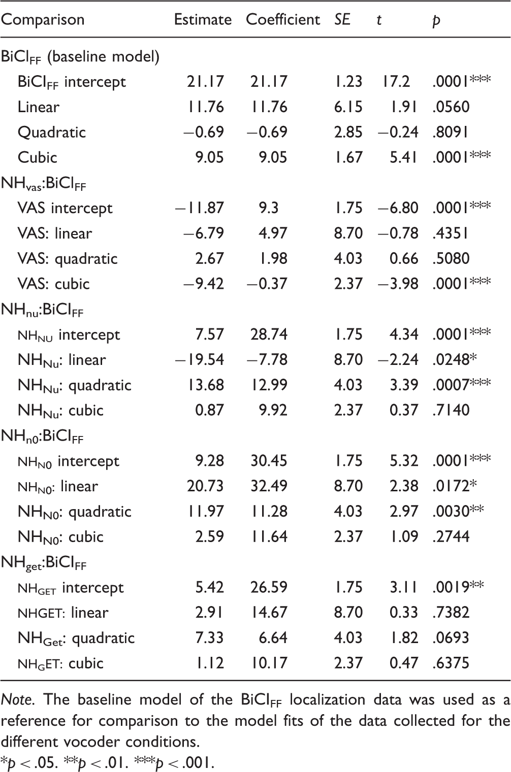
For statistical analysis using orthogonal polynomials, the intercept component corresponds to the overall average of the measure of interest (Mirman, 2014), which in this study was the absolute error. First, there was a significant effect of the BiCI_FF condition on the intercept component, indicating that this condition resulted in an absolute error (21.17°) that was significantly different from an absolute error of 0°(see Table 3). Next, the intercept components were compared across conditions. Conceptually, this is roughly like a t test comparing the tested conditions to the baseline model (Mirman, 2014). For example, the average absolute error for the NH_VAS condition was 11.87° less than the BiCI_FF condition, which was found to be significant, and the average absolute error for the NH_Nu condition was 7.57° greater than the BiCI_FF condition, which was also significant (see Table 3). All the NH listening conditions resulted in significant intercept effects, which indicate that the average absolute error for the NH conditions was significantly different than the BiCI_FF condition. That is, the average absolute localization error in BiCI users was significantly higher than the NH_VAS condition and significantly lower than all three of the NH vocoder conditions.

The first-order polynomial is the linear component and describes the slope of the relationship between absolute target and absolute error. There were significant linear effects for all of the vocoder conditions, except for the NH_Nu condition, meaning that as the absolute target angle increased, the absolute error increased. The NH_N0 condition had a significantly larger linear effect compared with the BiCI_FF model, as can be observed in the steeper slope (Figure 3, NH_N0 panel). The linear components of the NH_VAS and NH_GET fits were not significantly different than the linear component of the BiCI_FF fit (see Table 3, Condition:Linear for statistical summary).

Apart from the differences in slope, there were differences in the degree of curvature which were captured by the second-order polynomial. This is the quadratic component and describes the degree of slope change (i.e., single inflection) in the data. The quadratic components of the NH_Nu and NH_N0 conditions were significantly different than those from the BiCI_FF data. The NH_VAS, NH_GET, and BiCI_FF conditions were similar in that they all lacked a significant quadratic effect (see Table 3, Condition:Quadratic for statistical summary).

One of the more interesting findings of this study was that the BiCI and vocoder conditions exhibited an additional inflection that was not observed in the NH_VAS model. This is captured by the cubic component (i.e., third-order polynomial) and indicates the degree of a second inflection in a curve. Specifically, the cubic component describes the dip in the response curve around the 60° target angle, which did not emerge in the NH_VAS condition (Figure 3, NH_VAS panel compared with all other panels). This indicates that the error rates proximal to 60° were smaller for both NH listeners (vocoded conditions) and BiCI users. Overall, the main finding of the multilevel regression analysis was that the NH_GET condition produced localization performance that was most similar to that measured in BiCI users.

Interestingly, there was noticeable intersubject variability with regard to how NH subjects performed on the same vocoder conditions. To illustrate the various patterns of response distributions observed for different subjects, we show the NH_GET condition, which was found to be most comparable to BiCI_FF performance (see earlier). Figure 4 compares individual localization data for six BiCI subjects (Figure 4(a) to (c)) and six NH subjects (Figure 4(d) to (f)). The overall RMS error for each condition is shown inside each plot (see bottom right), where smaller values indicate better localization performance. Qualitatively, responses falling on the positive sloping diagonal are indicative of accurate localization. For visual comparison between NH_GET and BiCI_FF response distributions, response histograms are plotted on the right of each figure. Data from these subjects were chosen to depict the variability observed in performance across NH subjects for the vocoded stimuli (see NH_GET, Figure 4(b)) that coincided with the variability observed in BiCI_FF response distributions. Similar response distributions are plotted in each column. For example, the two BiCI subjects (Figure 4(a)) and the two NH subjects (Figure 4(b)) in the first column distributed responses to more central locations. The center column (Figure 4(b) and (e)) shows subjects whose majority of responses were grouped around spatial locations on either side. The column on the far right (Figure 4(c) and (f)) shows distribution patterns in which the majority of responses grouped into three spatial locations (i.e., left, center, and right). The similar variability in response distributions for both NH subjects listening to NH_GET stimuli and for BiCI subjects listening in the FF suggest that individuals distribute responses differently given degraded auditory input whether the signal is acoustically degraded or presented via electrical stimulation.

Figure 4.

Localization data and response distributions. Responses were binned to the nearest 10° and data point size reflects the number of responses within each bin (bottom left). The number at the bottom right corner of each plot is the RMS error. The small bar graphs next to each localization plot display a histogram of responses binned to the nearest 10°. (a–c) Localization data measured in BiCI users who responses varied by grouping around different spatial location. (d–f) Localization data in NH subjects who exhibited similar patterns of response distributions listening to VC_GET stimuli as the BiCI users in the column above them.

Discussion

The experiments reported here tested the ability of NH listeners to localize VAS stimuli that were processed through noise and GET vocoders for sounds varying in location along the horizontal plane. The present study demonstrates that NH localization performance along the horizontal plane can be degraded to levels observed in BiCI patients using a combination of VAS and vocoder techniques. The results showed that sound localization performance was significantly worse for all vocoded stimuli compared with virtual FF stimuli (Figure 1); thus, a detrimental effect on NH performance occurs with vocoders and degrades performance of individuals with healthy auditory systems to similar levels of horizontal-plane localization observed in BiCI users. In particular, the GET vocoder provided the best simulation of BiCI FF performance across the population of NH subjects tested here (Figure 3). An additional interesting finding is that NH listeners exhibited a similar range of intersubject variability and error patterns as was observed in BiCI subjects (Figure 4). These observations suggest that human listeners vary in how they process and localize degraded auditory inputs, regardless of whether the cause of degradation in the signal is due to the signal processing imposed on acoustic signals or due to the numerous factors that impact signals when they are provided electrically. Although both BiCI listeners and NH subjects listening to the vocoded stimuli exhibited variable response distributions, there was an observable inflection point around the ±60° in the average error patterns across locations for each of these groups (Figure 3). This inflection can also be observed in the lower errors (Figure 2(a)) and the increase in responses for these locations (Figure 2(b)), such that we speculate listeners may be responding to these locations when they are unsure of the exact source location but are confident that the sound originated from a location somewhere in that particular hemifield.

Localization performance measured here for the BiCI subjects was comparable to previously reported BiCI data (Grantham et al., 2007; Grieco-Calub & Litovsky, 2010; Litovsky et al., 2009; Majdak et al., 2011; Nopp et al., 2004). Grantham et al. (2007) reported an average overall error of 29.1 ± 7.6° for 22 BiCI users localizing speech stimuli. Similarly, Litovsky et al. (2009) reported overall localization errors of 28.4 ± 12.5° for 17 postlingually deafened BiCI users. More recently, localization of virtual sound sources has been reported for five BiCI users with an average precision error of 23.4 ± 2.3° for noise stimuli roved at a similar level ( ± 5 dB) to our study (Majdak et al., 2011). The average across-subject RMS error and response variability measured in BiCI subjects in the present study (27.9 ± 12.3°) is consistent with these previous findings. Interestingly, despite all the disadvantages that BiCI users face (i.e., independently functioning devices, reduced spectral information, current spread, electrode mismatch, varying etiologies, and amounts of neural degeneration), the average RMS for these listeners was lower than the NH average RMS for all three vocoder conditions. One possible reason for these lower RMS errors could be the stimuli used to test BiCI localization. The pink noise stimuli may have provided additional directional information, and were repeated four times, providing multiple looks. Another reason for the lower overall RMS error in BiCI users may be because these listeners had more experience with degraded auditory input, as all the BiCI subjects had a minimum of 1 year of listening experience with their CIs, whereas NH subjects were tested acutely. Goupell, et al. (2010) demonstrated that NH localization along the median plane while listening to GET-vocoded VAS stimuli significantly improved with training, although the performance was not as accurate as listening to unprocessed stimuli. Thus, it is reasonable to hypothesize that with more experience, the NH subjects in this study could possibly exhibit performance that would be similar to the overall RMS errors measured in the BiCI subjects.

The large increase in overall localization errors for NH subjects listening to vocoded stimuli occurred whether the original signal’s acoustic TFS was replaced with uncorrelated (NH_Nu), correlated (NH_N0), or synchronized-pulsatile (NH_GET) stimulation. Replacing the acoustic TFS during CI speech encoding creates binaural stimulation in which the TFS-ITDs that are presented to the auditory system do not correspond with the ILDs presented, and results in conflicting acoustical cues (i.e., each cue points to a different location). Studies show that when presenting the NH auditory system with conflicting ITD and ILD cues via VAS techniques, both the neural representation of these cues (Delgutte, Joris, Litovsky, & Yin, 1999; Slee & Young, 2011; Sterbing, Hartung, & Hoffmann, 2003) and localization performance (Macpherson & Middlebrooks, 2002; Middlebrooks, 1999; Middlebrooks, Macpherson, & Onsan, 2000; Wightman & Kistler, 1992) become altered compared with when the cues are consistent with how they are naturally experienced. In the present study for instance, the acoustic carriers in the vocoder stimuli would still activate the neural circuitry responsible for extracting ITDs; however, as they do not contain the acoustically appropriate ITD information, a neural representation of inconsistent ITD/ILD cues is more than likely to be encoded. In fact, binaural interference may occur in which the acoustically inappropriate low-frequency ITDs would dominate an individual’s perceived lateral position (Best, Gallun, Carlile, & Shinn-Cunningham, 2007; Best, Laback, & Majdak, 2011) and may be responsible for the inaccurate localization observed in both BiCI users and NH subjects listening to vocoded stimuli. Although auditory deprivation has been shown to result in degraded sound localization (Noble, Byrne, & Lepage, 1994), the extent to which degraded neural circuitry in BiCI users is responsible for poor localization has not been previously studied. Because we observed similar localization deficits in individuals with intact auditory systems listening to BiCI simulations (Figure 4), we posit that horizontal-plane localization deficits are attributable to the signal processing in CIs more so than the compromised auditory systems of BiCI users.

The experimental approaches reported here aimed to simulate the effects of various aspects CI speech encoding and bilateral stimulation on horizontal-plane sound localization. One issue may be that the independent signal processing, variable channel selection, and high-rate electrical stimulation introduces interaural decorrelation into the signals presented to the auditory system, in addition to impeding the ability to deliver ITD information (Seeber & Fastl, 2008). A likely consequence is that the spectrotemporal representations of acoustic signals are not being presented at the two ears with a high amount of binaural coherence. Several studies in NH listeners have reported that a reduction in the interaural correlation is perceived by the listener as a broadening of the sound image (Bernstein & Trahiotis, 1992; Durlach, Gabriel, Colburn, & Trahiotis, 1986; Gabriel & Colburn, 1981; Goupell & Hartmann, 2006; Jeffress, Blodgett, & Deatherage, 1962). The NH_Nu stimuli in the present study simulated this potential reduction in interaural correlation due to independent signal processing and variable channel selection. Additionally, the NH_N0 stimuli tested whether localization could be improved by creating of a more punctuate sound image via the temporal synchronization of the spectrally random carriers across the ears.

Comparing the performance between the two noise-vocoded conditions (Figure 3, NH_Nu and NH_N0 panels), the NH_Nu stimuli resulted in extremely poor localization across all azimuthal locations. In contrast, localization of the NH_N0 stimuli was biased toward the speaker location at 0° (Figure 2(a) and (b)) and rapidly decreased at more lateral positions. The NH_Nu data are in agreement with previous psychoacoustical studies, which have demonstrated that as the signal correlation between the ears decreases, the perceived sound image becomes more diffused and lateralization abilities deteriorate (Bernstein & Trahiotis, 1997; Goupell & Hartmann, 2006; Goupell & Litovsky, 2013; Jeffress et al., 1962; Trahiotis, Bernstein, Stern, & Buell, 2005). In addition to this, neural ITD encoding of broadband signals, such as speech, depends critically on a high amount of binaural coherence in the spectrotemporal features of the acoustic signals (Egnor, 2001; Saberi et al., 1998). Saberi et al. (1998) investigated the effects of binaural decorrelation on neural spatial coding and behavioral responses to spatial cues in the barn owl. Localization performance in barn owls for noise burst containing ITDs (and no ILDs) rapidly deteriorated as the interaural correlation of the signals presented was decreased (Saberi et al., 1998). Furthermore, responses of ITD sensitive neurons in the owl’s optic tectum declined rapidly as interaural decorrelation increased, thus these neurons exhibited less ITD tuning to the decorrelated stimuli. Similar findings have been shown in human cortical imaging studies (Zimmer & Macaluso, 2005, 2009). Zimmer and Macaluso (2005) found that activity in Heshl’s gyrus increased with increasing interaural correlation of white noise stimuli and that posterior auditory regions also showed increased activity for the high coherence stimuli, primarily when sound localization was being performed. Thus, the lack of interaural correlation in the NH_Nu stimuli may explain why these stimuli were difficult to localize.

For the NH_N0 stimuli, although the signals were completely correlated between the ears, the dominant low-frequency TFS-ITD cues contained in each of the stimuli across all spatial locations pointed to the center. Thus, the pattern of errors (Figure 3, NH_N0 panel) for this condition, that is, the higher degree of errors for more lateral locations, can be explained because subjects on average perceived the sound image to be coming from more central locations (Figure 2(b)). In the studies mentioned earlier (Egnor, 2001; Saberi et al., 1998; Zimmer & Macaluso, 2005, 2009), ITDs were applied to stimuli with various degrees of correlation between completely uncorrelated (N_u) and correlated (N₀) noise tokens. Here, we were also able to investigate whether applying individualized HRTF filtering (i.e., containing all the natural acoustical cues) and physiologically meaningful temporal envelopes (i.e., speech) to the N_u and N₀ noise carriers could produce accurate sound localization. Previous studies have investigated the contribution of envelope ITDs cues to intracranial lateralization in NH listeners (Bernstein & Trahiotis, 1996, 2002; Dietz, Ewert, & Hohmann, 2009, 2011; Laback, Zimmermann, Majdak, Baumgartner, & Pok, 2011). However, Dietz et al., (2011) also reported that auditory model predictions of localization accuracy based solely on envelope modulations were worse than the predictions based on fine structure. Our data are in agreement with this study, demonstrating that ITD cues in the envelopes of FF speech stimuli are not sufficient in moving the NH_N0 sound image across the spatial locations.

The GET vocoder was used to simulate the electrical pulse trains delivered during CI stimulation. Similar techniques to those reported here have been used previously to test sound localization in the median plane (Goupell et al., 2010). Given the extensive literature on lateralization/discrimination of ITDs in amplitude-modulated stimuli (Bernstein & Trahiotis, 1985, 2002; Laback, Pok, et al., 2004; Laback, Zimmermann, et al., 2011; Seeber & Fastl, 2008; Van Hoesel et al., 2009), one could speculate that the temporal modulations of speech envelopes would provide an additional cue for sound localization in the horizontal plane. Although the ability of BiCI users to perform sound localization tasks based solely on envelope ITDs has not been investigated directly, their ability to discriminate and lateralize such stimuli has been studied (Ihlefeld, Kan, & Litovsky, 2014; Laback, Pok, et al., 2004, Laback, Zimmermann, et al., 2011; Van Hoesel et al., 2009). Laback, Pok, et al. (2004) showed that the best envelope ITD thresholds in BiCI users were on the order of 150 µs and that envelope ITDs could induce monotonic changes in the lateralization of the auditory image. It should also be noted that the ITD thresholds measured for click trains were significantly lower than for speech tokens. However, previous studies do not indicate that envelope ITD sensitivity will translate into accurate localization of FF sound sources.

Our study differs from previous amplitude-modulated ITDs studies in two ways. First, the listening task and spatial hearing assessments were different, as previous studies measured either ITD discrimination or intracranial lateralization of stimuli containing independent fine-structure and envelope-based temporal disparities. Second, prior studies used periodic carriers with periodic modulators and 100% modulation depths. For speech, however, signals are more complex with envelope modulations that are shallower and less temporally consistent relative to the modulators use in fixed-frequency stimuli. In addition, the filtering by HRTFs (i.e., the frequency-dependent ILDs) further affects the depths of the ongoing envelope temporal modulations between the ears. Reducing the depth of envelope modulations has been shown to result in poorer ITD thresholds (Bernstein & Trahiotis, 1996; Ihlefeld et al., 2014). Our findings lend support to this notion, as the temporal envelope cues available to the NH subjects listening to GET vocoder simulations did not appear to provide sufficient information to produce accurate sound localization (Figure 3, NH_GET panel). However, the similar patterns in errors across azimuthal locations suggest that the NH_GET stimuli produced the most comparable performance to BiCI localization in NH listeners.

The variability in performance observed for both BiCI and NH listeners (Figure 4) suggests that the localization strategies used by individuals are different, whether auditory signals are degraded acoustically or provided electrically. Recent studies involving sound source identification (i.e., ability of listeners to identify objects from the sound of impact) in quiet have shown that listeners regularly use different listening strategies that result in similar performance accuracy, but for different levels of variability in performance (Lutfi & Liu, 2007; Lutfi, Liu, & Stoelinga, 2011). The current study suggests a similar notion for sound localization of degraded auditory signals. For example, BiCI subjects ICF, ICO, and IBY (Figure 4(a) to (c)) had similar overall RMS error (∼ 25 – 26°), but very different response distributions. Although such intersubject variability is often attributable to the fact that these listeners used BiCIs for hearing, it was observed that NH listeners also exhibited similar variability when listening to vocoder processed stimuli. For instance, NH subjects STL and TAQ (Figure 4(d) and (e), respectively) had similar overall RMS errors (∼ 38 – 39°), but the errors were accounted for by very different error distributions. While subject STL responded to mostly central locations, TAQ distributed responses around left and right locations. Such observations indicate that the intersubject variability observed for BiCI users may not solely reflect factors that are often considered to be the root of localization errors, such as peripheral factors, but may be the result of individuals employing different strategies for making decisions about the location of a sound source when given degraded auditory input.

Conclusion

Simulated CI speech encoding resulted in large sound localization deficits in NH listeners, and overall errors were comparable with those measured in bilaterally implanted patients.

Among the vocoders used to process free-field speech envelopes, the GET vocoder produced the most similar patterns of localization error across azimuth to those observed in BiCI users.

Although these data were obtained with CI simulations, they nonetheless lend support to the notion that CI speech encoding in the present day bilateral listening mode contributes to sound localization difficulties in BiCI users. The crux of this finding assumes that the bilateral vocoder simulations described in this study approximate the interaural cues available to the binaural circuits of BiCI users; however, the integrity with which binaural cues are preserved at the level of binaural neural circuitry is currently unknown, and more than likely varies across patient and devices type.

NH listeners exhibited a similar intersubject variability in error patterns to that observed in the BiCI users, suggesting that individuals employ different strategies when identifying a sound source location whether auditory signals are degraded acoustically or provided electrically.

Future studies using the techniques presented here could efficiently investigate the potential success of novel sound encoding strategies aimed at improving spatial hearing abilities in bilaterally implanted patients.

Footnotes

Declaration of Conflicting Interests

The authors declared no potential conflicts of interest with respect to the research, authorship, and/or publication of this article.

Funding

The authors disclosed receipt of the following financial support for the research, authorship, and/or publication of this article: This study was supported by grants from the NIH-NIDCD (R01 DC003083 and R01 DC01049) and in part by a core grant from the NIH-NICHD to the Waisman Center (P30 HD03352).

Acknowledgements

We would like to thank all our listeners who participated in these experiments, Kyle Martel and Kate Landowski for all their help with data collection, and Amy Jones and Ann Todd for providing review and feedback on prior drafts of the manuscript. We would like to especially thank Dr. Matt Winn for providing assistance with coding the R software and his thoughtful discussions on data interpretation.

References

Bernstein

L. R.

Trahiotis

(1985) Lateralization of sinusoidally amplitude-modulated tones: Effects of spectral locus and temporal variation. The Journal of the Acoustical Society of America 78(2): 514–523.

Bernstein

L. R.

Trahiotis

(1992) Discrimination of interaural envelope correlation and its relation to binaural unmasking at high frequencies. The Journal of the Acoustical Society of America 91(1): 306–316.

Bernstein

L. R.

Trahiotis

(1996) On the use of the normalized correlation as an index of interaural envelope correlation. The Journal of the Acoustical Society of America 100(3): 1754–1763.

Bernstein

L. R.

Trahiotis

(1997) The effects of randomizing values of interaural disparities on binaural detection and on discrimination of interaural correlation. The Journal of the Acoustical Society of America 102(2 Pt. 1): 1113–1120.

Bernstein

L. R.

Trahiotis

(2002) Enhancing sensitivity to interaural delays at high frequencies by using “transposed stimuli”. The Journal of the Acoustical Society of America 112(3 Pt. 1): 1026–1036.

Best

Gallun

F. J.

Carlile

Shinn-Cunningham

B. G.

(2007) Binaural interference and auditory grouping. The Journal of the Acoustical Society of America 121(2): 1070–1076.

Best

Laback

Majdak

(2011) Binaural interference in bilateral cochlear-implant listeners. The Journal of the Acoustical Society of America 130(5): 2939–2950. doi:10.1121/1.3641400.

Bingabr

Espinoza-Varas

Loizou

P. C.

(2008) Simulating the effect of spread of excitation in cochlear implants. Hearing Research 241(1–2): 73–79. doi:10.1016/j.heares.2008.04.012.

Blauert

(1997) Spatial hearing: The psychophysics of human sound localization 2nd ed, vol. 36–200.Cambridge, MA: MIT Press.

10.

Coco

Epp

S. B.

Fallon

J. B.

Millard

R. E.

Shepherd

R. K.

(2007) Does cochlear implantation and electrical stimulation affect residual hair cells and spiral ganglion neurons? Hearing Research 225(1–2): 60–70. doi:S0378-5955(06)00337-6 [pii] 10.1016/j.heares.2006.12.004.

11.

Crew

J. D.

Galvin

J. J.

Q.-J.

(2012) Channel interaction limits melodic pitch perception in simulated cochlear implants. The Journal of the Acoustical Society of America 132(5): EL429–EL435. doi:10.1121/1.4758770.

12.

Delgutte

Joris

P. X.

Litovsky

R. Y.

Yin

T. C.

(1999) Receptive fields and binaural interactions for virtual-space stimuli in the cat inferior colliculus. Journal of Neurophysiology 81(6): 2833–2851.

13.

Dietz

Ewert

S. D.

Hohmann

(2009) Lateralization of stimuli with independent fine-structure and envelope-based temporal disparities. The Journal of the Acoustical Society of America 125(3): 1622–1635. doi:10.1121/1.3076045.

14.

Dietz

Ewert

S. D.

Hohmann

(2011) Auditory model based direction estimation of concurrent speakers from binaural signals. Speech Communication 53(5): 592–605.

15.

Dorman

M. F.

Loizou

P. C.

(1997) Speech intelligibility as a function of the number of channels of stimulation for normal-hearing listeners and patients with cochlear implants. The American Journal of Otology 18(6 Suppl): S113–S114.

16.

Dorman

M. F.

Loizou

P. C.

Fitzke

(1998) The identification of speech in noise by cochlear implant patients and normal-hearing listeners using 6-channel signal processors. Ear and Hearing 19(6): 481–484.

17.

Dorman

M. F.

Loizou

P. C.

Fitzke

(1998) The recognition of sentences in noise by normal—hearing listeners using simulations of cochlear-implant signal processors with 6-20 channels. The Journal of the Acoustical Society of America 104(6): 3583–3585.

18.

Dorman

M. F.

Loizou

P. C.

Rainey

(1997) Simulating the effect of cochlear-implant electrode insertion depth on speech understanding. The Journal of the Acoustical Society of America 102(5 Pt. 1): 2993–2996.

19.

Durlach

N. I.

Gabriel

K. J.

Colburn

H. S.

Trahiotis

(1986) Interaural correlation discrimination: II. Relation to binaural unmasking. The Journal of the Acoustical Society of America 79(5): 1548–1557.

20.

Egnor

S. E.

(2001) Effects of binaural decorrelation on neural and behavioral processing of interaural level differences in the barn owl (Tyto alba). The Journal of Comparative Physiology A 187(8): 589–595.

21.

Q. J.

Nogaki

(2005) Noise susceptibility of cochlear implant users: The role of spectral resolution and smearing. Journal of the Association for Research in Otolaryngology 6(1): 19–27. doi:10.1007/s10162-004-5024-3.

22.

Gabriel

K. J.

Colburn

H. S.

(1981) Interaural correlation discrimination: i. bandwidth and level dependence. The Journal of the Acoustical Society of America 69(5): 1394–1401.

23.

Goupell

M. J.

Hartmann

W. M.

(2006) Interaural fluctuations and the detection of interaural incoherence: Bandwidth effects. The Journal of the Acoustical Society of America 119(6): 3971–3986.

24.

Goupell

M. J.

Litovsky

R. Y.

(2013) The effect of interaural fluctuation rate on correlation change discrimination. Journal of the Association for Research in Otolaryngology 15(1): 115–129. doi:10.1007/s10162-013-0426-8.

25.

Goupell

M. J.

Majdak

Laback

(2010) Median-plane sound localization as a function of the number of spectral channels using a channel vocoder. The Journal of the Acoustical Society of America 127(2): 990–1001. doi:10.1121/1.3283014.

26.

Goupell

M. J.

Stoelb

Kan

Litovsky

R. Y.

(2013) Effect of mismatched place-of-stimulation on the salience of binaural cues in conditions that simulate bilateral cochlear-implant listening. The Journal of the Acoustical Society of America 133(4): 2272–2287. doi:10.1121/1.4792936.

27.

Grantham

D. W.

Ashmead

D. H.

Ricketts

T. A.

Labadie

R. F.

Haynes

D. S.

(2007) Horizontal-plane localization of noise and speech signals by postlingually deafened adults fitted with bilateral cochlear implants. Ear and Hearing 28(4): 524–541. doi:10.1097/AUD.0b013e31806dc21a 00003446-200708000-00009 [pii].

28.

Greenwood

D. D.

(1990) A cochlear frequency-position function for several species—29 years later. The Journal of the Acoustical Society of America 87(6): 2592–2605.

29.

Grieco-Calub

T. M.

Litovsky

R. Y.

(2010) Sound localization skills in children who use bilateral cochlear implants and in children with normal acoustic hearing. Ear and Hearing 31(5): 645–656. doi:10.1097/AUD.0b013e3181e50a1d.

30.

Hinojosa

Marion

(1983) Histopathology of profound sensorineural deafness. Annals of the New York Academy of Sciences 405: 459–484.

31.

Ihlefeld, A., Kan, A., & Litovsky, R. Y. (2014). Across-frequency combination of interaural time difference in bilateral cochlear implant listeners. Frontiers in Systems Neuroscience, 8, 22. doi:10.3389/fnsys.2014.00022.

32.

Jeffress

L. A.

Blodgett

H. C.

Deatherage

B. H.

(1962) Effect of interaural correlation on the precision of centering a noise. The Journal of the Acoustical Society of America 34(8): 1122–1123.

33.

Kan

Stoelb

Litovsky

R. Y.

Goupell

M. J.

(2013) Effect of mismatched place-of-stimulation on binaural fusion and lateralization in bilateral cochlear-implant users. The Journal of the Acoustical Society of America 134(4): 2923–2936. doi:10.1121/1.4820889.

34.

Laback

Pok

S. M.

Baumgartner

W. D.

Deutsch

W. A.

Schmid

(2004) Sensitivity to interaural level and envelope time differences of two bilateral cochlear implant listeners using clinical sound processors. Ear and Hearing 25(5): 488–500. doi:00003446-200410000-00008 [pii].

35.

Laback

Zimmermann

Majdak

Baumgartner

W.-D.

Pok

S.-M.

(2011) Effects of envelope shape on interaural envelope delay sensitivity in acoustic and electric hearing. The Journal of the Acoustical Society of America 130(3): 1515–1529. doi:10.1121/1.3613704.

36.

Landsberger

D. M.

Padilla

Srinivasan

A. G.

(2012) Reducing current spread using current focusing in cochlear implant users. Hearing Research 284(1–2): 16–24. doi:S0378-5955(11)00302-9 [pii] 10.1016/j.heares.2011.12.009.

37.

Leake

P. A.

Hradek

G. T.

Snyder

R. L.

(1999) Chronic electrical stimulation by a cochlear implant promotes survival of spiral ganglion neurons after neonatal deafness. Journal of Comparative Neurology 412(4): 543–562. doi:10.1002/(SICI)1096-9861(19991004)412:4<543::AID-CNE1>3.0.CO;2-3 [pii].

38.

Litovsky

R. Y.

(2011) Review of recent work on spatial hearing skills in children with bilateral cochlear implants. Cochlear Implants International 12(Suppl. 1): S30–S34. doi:10.1179/146701011X13001035752372.

39.

Litovsky

R. Y.

Goupell

M. J.

Godar

Grieco-Calub

Jones

G. L.

Garadat

S. N.

Misurelli

(2012) Studies on bilateral cochlear implants at the University of Wisconsin’s Binaural Hearing and Speech Laboratory. The Journal of the American Academy of Audiology 23(6): 476–494. doi:10.3766/jaaa.23.6.9.

40.

Litovsky

R. Y.

Jones

G. L.

Agrawal

van Hoesel

(2010) Effect of age at onset of deafness on binaural sensitivity in electric hearing in humans. The Journal of the Acoustical Society of America 127(1): 400–414. doi:10.1121/1.3257546.

41.

Litovsky

R. Y.

Parkinson

Arcaroli

(2009) Spatial hearing and speech intelligibility in bilateral cochlear implant users. Ear and Hearing 30(4): 419–431. doi:10.1097/AUD.0b013e3181a165be.

42.

Loizou

P. C.

(1999) Signal-processing techniques for cochlear implants. IEEE Engineering in Medicine and Biology Magazine 18(3): 34–46.

43.

Lutfi

R. A.

Liu

C. J.

(2007) Individual differences in source identification from synthesized impact sounds. The Journal of the Acoustical Society of America 122(2): 1017–1028. doi:10.1121/1.2751269.

44.

Lutfi

R. A.

Liu

C. J.

Stoelinga

C. N.

(2011) Auditory discrimination of force of impact. The Journal of the Acoustical Society of America 129(4): 2104–2111. doi:10.1121/1.3543969.

45.

Macpherson

E. A.

Middlebrooks

J. C.

(2002) Listener weighting of cues for lateral angle: the duplex theory of sound localization revisited. The Journal of the Acoustical Society of America 111(5): 2219–2236.

46.

Majdak

Goupell

M. J.

Laback

(2011) Two-dimensional localization of virtual sound sources in cochlear-implant listeners. Ear and Hearing 32(2): 198–208. doi:10.1097/AUD.0b013e3181f4dfe9.

47.

Majdak

Laback

Baumgartner

W. D.

(2006) Effects of interaural time differences in fine structure and envelope on lateral discrimination in electric hearing. The Journal of the Acoustical Society of America 120(4): 2190–2201.

48.

Middlebrooks

J. C.

(1999) Individual differences in external-ear transfer functions reduced by scaling in frequency. The Journal of the Acoustical Society of America 106(3 Pt. 1): 1480–1492.

49.

Middlebrooks

J. C.

Green

D. M.

(1991) Sound localization by human listeners. Annual Review of Psychology 42: 135–159. doi:10.1146/annurev.ps.42.020191.001031.

50.

Middlebrooks

J. C.

Macpherson

E. A.

Onsan

Z. A.

(2000) Psychophysical customization of directional transfer functions for virtual sound localization. Journal of the Acoustical Society of America 108(6): 3088–3091.

51.

Mirman

(2014) Growth curve analysis and visualization using R, New York, NY: Chapman and Hall/CRC Press.

52.

Møller

(1992) Fundamentals of binaural technology. Applied Acoustics 36(3-4): 171–218.

53.

Nadol

J. B.

Jr. Young

Y. S.

Glynn

R. J.

(1989) Survival of spiral ganglion cells in profound sensorineural hearing loss: implications for cochlear implantation. Annals of Otology, Rhinology & Laryngology 98(6): 411–416.

54.

Noble

Byrne

Lepage

(1994) Effects on sound localization of configuration and type of hearing impairment. The Journal of the Acoustical Society of America 95(2): 992–1005.

55.

Nopp

Schleich

D’Haese

(2004) Sound localization in bilateral users of MED-EL COMBI 40/40+ cochlear implants. Ear and Hearing 25(3): 205–214. doi:00003446-200406000-00002 [pii].

56.

Otte

Schunknecht

H. F.

Kerr

A. G.

(1978) Ganglion cell populations in normal and pathological human cochleae. Implications for cochlear implantation. Laryngoscope 88(8 Pt. 1): 1231–1246. doi:10.1288/00005537-197808000-00004.

57.

Qin

M. K.

Oxenham

A. J.

(2003) Effects of simulated cochlear-implant processing on speech reception in fluctuating maskers. The Journal of the Acoustical Society of America 114(1): 446–454.

58.

Saberi

Takahashi

Konishi

Albeck

Arthur

B. J.

Farahbod

(1998) Effects of interaural decorrelation on neural and behavioral detection of spatial cues. Neuron 21(4): 789–798. doi:S0896-6273(00)80595-4 [pii].

59.

Seeber

B. U.

Baumann

Fastl

(2004) Localization ability with bimodal hearing aids and bilateral cochlear implants. The Journal of the Acoustical Society of America 116(3): 1698–1709.

60.

Seeber

B. U.

Fastl

(2008) Localization cues with bilateral cochlear implants. The Journal of the Acoustical Society of America 123(2): 1030–1042. doi:10.1121/1.2821965.

61.

Shannon

R. V.

Zeng

F. G.

Kamath

Wygonski

Ekelid

(1995) Speech recognition with primarily temporal cues. Science 270(5234): 303–304.

62.

Slee

S. J.

Young

E. D.

(2011) Information conveyed by inferior colliculus neurons about stimuli with aligned and misaligned sound localization cues. Journal of Neurophysiology 106(2): 974–985. doi:jn.00384.2011 [pii] 10.1152/jn.00384.2011.

63.

Sterbing

S. J.

Hartung

Hoffmann

K. P.

(2003) Spatial tuning to virtual sounds in the inferior colliculus of the guinea pig. Journal of Neurophysiology 90(4): 2648–2659.

64.

Trahiotis

Bernstein

L. R.

Stern

R. M.

Buell

T. N.

(2005) Interaural correlation as the basis of a working model of binaural processing: an introduction. In: Popper

A. N.

Fay

R. R.

(eds) Sound source localization, springer handbook of auditory research Vol. 25.New York, NY: Springer, pp. 238–271. doi:10.1007/0-387-28863-5_7.

65.

van Hoesel

Ramsden

Odriscoll

(2002) Sound-direction identification, interaural time delay discrimination, and speech intelligibility advantages in noise for a bilateral cochlear implant user. Ear and Hearing 23(2): 137–149.

66.

van Hoesel

R. J.

(2004) Exploring the benefits of bilateral cochlear implants. Audiology and Neurotology 9(4): 234–246. doi:10.1159/000078393 78393 [pii].

67.

van Hoesel

R. J.

(2007) Sensitivity to binaural timing in bilateral cochlear implant users. The Journal of the Acoustical Society of America 121(4): 2192–2206.

68.

van Hoesel

R. J.

(2008) Observer weighting of level and timing cues in bilateral cochlear implant users. The Journal of the Acoustical Society of America 124(6): 3861–3872. doi:10.1121/1.2998974.

69.

van Hoesel

R. J.

Jones

G. L.

Litovsky

R. Y.

(2009) Interaural time-delay sensitivity in bilateral cochlear implant users: Effects of pulse rate, modulation rate, and place of stimulation. Journal of the Association for Research in Otolaryngology 10(4): 557–567. doi:10.1007/s10162-009-0175-x.

70.

van Hoesel

R. J.

Tyler

R. S.

(2003) Speech perception, localization, and lateralization with bilateral cochlear implants. The Journal of the Acoustical Society of America 113(3): 1617–1630.

71.

van Schijndel

N. H.

Houtgast

Festen

J. M.

(1999) Intensity discrimination of Gaussian-windowed tones: Indications for the shape of the auditory frequency-time window. The Journal of the Acoustical Society of America 105(6): 3425–3435.

72.

Wightman

F. L.

Kistler

D. J.

(1989) Headphone simulation of free-field listening. II: Psychophysical validation. The Journal of the Acoustical Society of America 85(2): 868–878.

73.

Wightman

F. L.

Kistler

D. J.

(1992) The dominant role of low-frequency interaural time differences in sound localization. Journal of the Acoustical Society of America 91(3): 1648–1661.

74.

Wilson

B. S.

Dorman

M. F.

(2008) Cochlear implants: Current designs and future possibilities. Journal of Rehabilitation Research and Development 45(5): 695–730.

75.

Wilson

B. S.

Finley

C. C.

Lawson

D. T.

Wolford

R. D.

Eddington

D. K.

Rabinowitz

W. M.

(1991) Better speech recognition with cochlear implants. Nature 352(6332): 236–238. doi:10.1038/352236a0.

76.

Zimmer

Macaluso

(2005) High binaural coherence determines successful sound localization and increased activity in posterior auditory areas. Neuron 47(6): 893–905. doi:S0896-6273(05)00613-6 [pii] 10.1016/j.neuron.2005.07.019.

77.

Zimmer

Macaluso

(2009) Interaural temporal and coherence cues jointly contribute to successful sound movement perception and activation of parietal cortex. Neuroimage 46(4): 1200–1208. doi:S1053-8119(09)00260-2 [pii] 10.1016/j.neuroimage.2009.03.022.

Comparing Sound Localization Deficits in Bilateral Cochlear-Implant Users and Vocoder Simulations With Normal-Hearing Listeners

Abstract

Keywords

Introduction

Methods

Participants

Equipment

HRTF Measurements

Stimuli

Nonvocoded stimuli

Vocoded stimuli

Testing Procedure

Results

Discussion

Conclusion

Footnotes

Declaration of Conflicting Interests

Funding

Acknowledgements

References