Sage Journals: Discover world-class research

Abstract

Point-based hierarchical Markov models for tennis provide transparency and flexibility in predicting the outcome and duration of matches, but have been shown to fall behind in predictive power compared to other methods such as regression. In this paper, a preliminary study is first conducted which highlights the point-based model’s preference for data quantity over quality with respect to time horizons and surface-filtering. Fixing these factors, the main study then ensembles point-based methods in the literature along with two novel methods, (i) using exclusively head-to-head (H2H) data and (ii) point-specific modifications, to significantly boost match outcome prediction accuracy. Consensus model ensembles, in particular, boost average prediction accuracies to around 70%, on par with machine learning models. Progress is also made in duration prediction with point-based models. Point-specific modifications and rudimentary mean duration ensembles show promise in lowering root mean squared error (RMSE), with the latter’s performance strongly correlated with outcome prediction strength for corresponding outcome prediction ensembles. Overall, the positive results speak to the continued relevance of more traditional probabilistic prediction methods and adds to the literature on the considerable potential in ensembling. Studies are conducted with data from professional men’s and women’s matches played during 2011-2022, with the years 2014, 2018, and 2022 set aside for testing.

Keywords

Tennis analytics markov chains absorption probability model ensembles tennis match outcome tennis match duration

Introduction

Involving only two players and having an exceptional amount of granular data collected on it, singles tennis is a sport that lends itself to modeling. This makes tennis a valuable testing site for new methods and ideas in sports analytics and prediction at large. The topic of tennis match outcome prediction, with potential in enhancing broadcast experiences, has only grown due to the proliferation of sports betting in North America. In addition to sports analytics researchers, broadcasters, viewers, and sports bettors, tennis practitioners are also among the beneficiaries of tennis modeling, as advances in tennis match outcome prediction work towards unlocking insights into the game’s implicit dynamics and patterns of play. A more dire problem in tennis analytics is that of predicting tennis match duration. Even for the most prestigious tennis tournaments, scheduling continues to be an issue, with otherwise high quality matches ending as late as five in the morning (Sten-Ziemons, 2024), harming tennis as a sport and as a product for players and fans alike.

As shall be seen in the subsequent literature review section, procedures employed to predict tennis match outcomes have developed from bookmaker consensus (Leitner et al., 2009) to machine learning methods, where the majority of recent advances are concentrated. The amount of literature is disproportionately lower with regards to tennis match duration prediction, though promising results using stochastic simulation (Kovalchik and Ingram, 2018; Lisi and Grigoletto, 2021) and machine learning (Duen and Peker, 2024) can still be found. Alternatively, prediction of both the outcome and duration of tennis matches can be approached through point-based Markov models for tennis, which emerged in the literature as early as 1970 with Schutz’s seminal work. This method makes use of the hierarchical structure of tennis: a match consists of sets, which consists of games, which consists of points. Therefore, under the assumption that points played in a match are conditionally independent and identically distributed (iid) given which player is serving, a model can be constructed, taking as input the two probabilities of each player winning their service point and outputting the probability a player wins the match.

Methods have been proposed to improve the prediction abilities of the point-based Markov model based on adjusting its input to account for the opponent’s return capability. The opponent-adjusted formula of Barnett and Clarke (2005) diminishes a player’s serve according to their opponent’s return statistics relative to the field, while the common opponent model of Knottenbelt et al. (2012) restricts the data used to only recent matches played against a list of common opponents. Kovalchik (2016) compares these techniques, amongst other point-based Markov model variations, with 2014 men’s tennis data, concluding that the opponent-adjusted formula outperforms the others, whilst highlighting a gap between the point-based models and the best of the regression-based models. Our study proposes and tests two additional methods, before applying ensembling techniques to bridge this gap. We test the performance of directly using head-to-head (H2H) data and also experiment with relaxing the identically distributed part of the model’s iid assumption, using a greedy algorithm to assign a subset of states in the point-to-game Markov model their own state-specific service point win probabilities. We then finally move to ensembling these individual models, including ones in the literature and our own two novel methods, to boost prediction accuracy for point-based Markov models. Several ensembling approaches are explored, but the consensus vote approach yields by far the most significant results, boosting the Markov model to be competitive with the best machine learning predictors. Running parallel to our study on outcome prediction, our work on match duration similarly begins with estimates yielded by the basic Markov model. Effect on duration prediction accuracy of all the individual modifications for outcome are examined, before moving on to ensembling results. Different from outcome prediction, improvements are now measured using root mean squared error (RMSE), with the time unit being minutes.

The improvements this paper makes to the prediction capabilities of the point-based Markov models can be summarized as follows:

Significantly boosts match outcome prediction accuracy through the ensembling of methods in the literature along with two novel methods. In particular, the consensus vote model with (i) common opponents, (ii) opponent-adjusted, (iii) opponent-adjusted common opponents, and (iv) point-specific activation components consistently and significantly outperforms opponent-adjusted models, and numerous ensemble models boost prediction accuracy to the level of the soft 70% ceiling for machine learning models found in Wilkens (2021).

Proposes and tests two novel modifications to the point-based Markov model: (i) directly using H2H data, and (ii) point-specific modifications to the model’s point-to-game layer. In particular, we find the former to increase accuracy on par with common opponents models, the latter to reduce duration RMSE on par with opponent-adjusted models, and both requiring more higher quality data for better predictions. Though not spectacular individually, both new models also prove to be important components to some of the best ensemble models.

Provides statistical evidence for conventional views on the effect of surface-filtering, time horizons, and change points on point-based models, as well as surface-filtered variations of Knottenbelt et al. (2012) common opponents model hitherto unexplored. Key conclusions from these preliminary studies are summarized in Appendix B, with the main study building on these results.

Through boosting the performance of point-based Markov models, and with further potential highlighted in terms of data granularity and player-specific changes, we aim to demonstrate the continued relevance of these approaches, adjacent to machine learning methods, which provide a high degree of transparency, enabling considerable explainability and customization.

The paper is organized as follows. “Literature Review” overviews the literature with regards to advances in both tennis match outcome and duration prediction. “Hierarchical IID Model” outlines the standard point-based Markov model under iid assumptions and how it is used for the prediction of tennis match outcomes and duration. Some related implementation details are left for Appendix A, along with some immediate results that can be derived from the model. “Data” details the data, how different sources were processed and used for different parts of the study. In “Individual Methods”, we expound on our new approaches, along with a note on variations of the common opponents approach that were not explored previously. “Ensemble Methods” overviews our ensembling methodologies. “Results and Discussion” presents and discusses experimental results for both outcomes and durations. “Concluding Remarks” contains a number of concluding remarks concerning the various studies conducted in the paper, along with potential future directions. Selected additional experimental results are organized in Appendix B, and code used for the entire study along with complete results can be viewed and downloaded at the GitHub repository “c567wang/Point-Based-Tennis-Prediction”.

Literature Review

Methods ranging from more traditional bookmaker consensus (Leitner et al., 2009) to machine learning methods employing regression (Clarke and Dyte, 2000) and neural networks (NNs) (Somboonphokkaphan et al., 2009), are overviewed and tested in studies such as Kovalchik (2016) and Wilkens (2021). The latter study, focusing purely on machine learning models, surveys NNs, logistic regression, random forests, gradient boosting machines, and support vector machines (SVMs), concludes after calibration that model accuracy rounds out at around 70% in the long run, the same accuracy as traditional bookmaker odds. Apart from the study’s experimentation results, this assertion reasons that the betting market already captures most information that can be used for prediction. Furthermore, Wilkens’ study examines the ensembling of the five aforementioned models, ranging from needing agreement from only a pair of models to full consensus, and producing comparatively encouraging betting results. More recent machine learning studies have continued to apply methods encompassed under Wilkens’ survey. Buhamra et al. (2024) focuses on regression models, while a follow-up study (Buhamra et al., 2025) expands the scope to other machine learning methods such as SVMs and XGBoost. Combined with feature engineering and intense calibration via cross-validation, the authors obtain accuracies around 77% for regression models, and accuracies up to 80% for NNs, all on 2022 Grand Slam matches. At the same time, the studies point to the importance of continuously incorporating match data from the Grand Slam closest to the time of prediction, in what they term an “expanding window” approach as opposed to “rolling windows”.

In contrast, Gupta and Assaf (2024) do not measure performance by accuracy, instead highlighting through the area-under-the-curve metric the prediction potential in using in-match statistics as features/predictors, while acknowledging that these would only be known post-match. (We conduct the same demonstration of predictive potential for the point-based models in “Individual methods”.) Jhawar (2022) tackles outcome prediction using k-means clustering, random forests, and multi-output regression on ATP data from 2000 to 2017, with random forests managing to reach 80% accuracy. Yue et al. (2022) explores the use of the Glicko rating system, evolving from the Elo ratings found in chess, for further feature engineering, in conjunction with logistic regression, SVMs, NNs, and gradient boosting. They achieve 70% accuracy on 2019 data and stress the superiority of player rankings as a feature. Though many of these later studies report accuracies over 70%, studies summarized and examined by Wilkens (2021) also reported accuracies exceeding 70% on their respective datasets. An updated survey focusing on the new machine learning models may be necessary to conduct rigorous comparisons and assessments, and it remains to be seen if more recent advances in parameter tuning, feature selection/engineering, and fresher training data closer to the time of prediction can consistently break through the proposed 70% ceiling.

Focusing now on the evolution of the point-based Markov model first introduced by Schutz (1970), there are two mathematically equivalent versions of this approach. The first uses combinatorial reasoning to derive sets of equations to represent the model (Adler and Ross, 2012; Newton and Keller, 2005; O’Donoghue and Simmonds, 2019), while the second models each level of the tennis match using discrete-time Markov chain (DTMC) theory. Winning probabilities and match duration estimates (and their distributions) can then be obtained via matrix inversion. Since it explicitly encapsulates the progression of a tennis match, the latter version lends itself to easier interpretation, examination, and modifications. The DTMC approach’s value in being able to concurrently predict match duration has been demonstrated by Barnett (2016), and was notably used in the 2014 book by Klaassen and Magnus, which consolidates years of the authors’ work on tennis, all based on a Markov chain iid model they named Richard. As described in “Introduction” and detailed further in “Individual methods”, the opponent-adjusted formula of Barnett and Clarke (2005) and the common opponent model of Knottenbelt et al. (2012) have been proposed for the point-based Markov model to account for the opponent’s return capability. Other point-based variations include the low-level point model of Spanias and Knottenbelt (2013) and the Bayesian hierarchical model of Ingram (2019). For our proposed point-specific modifications, a particular version of this has been considered by Carrari et al. (2017), where different parameters are estimated for pre-deuce and post-deuce states, whereas our study examines the entire point-to-game DTMC more systematically. Closely associated to relaxing the iid assumptions are the studies of Klaassen and Magnus (2014) and Sim and Choi (2020). However, these studies focus more on statistical significance while this study directly tests for effect on win prediction accuracy.

The literature is sparser on the side of match duration prediction. Aside from Barnett (2016), Kovalchik and Ingram (2018) and Lisi and Grigoletto (2021) have also examined the topic of match durations. However, these latter two studies fit distributions to match duration data to simulate matches, focusing more towards how rule changes would affect match lengths overall. The work of Duen and Peker (2024) marks an important milestone in duration prediction with the application of multi-linear regression, classification and regression trees (CARTs), support vector regression, and NNs to data from 1993 to 2022. Apart from CARTs, the other three approaches yield similarly admirable results, being off by an average of roughly 17.5 minutes for best-of-3 matches and 26 minutes for best-of-5 matches.

Methods

Hierarchical IID Model

We begin this section with some additional terminology and notation that will be used going forward. The main organizing bodies of professional tennis for men and women are the Association of Tennis Professionals (ATP) and the Women’s Tennis Association (WTA), respectively. We use “level” to refer to the hierarchical components of a tennis match. Specifically, these would be the point-to-game level, the game-to-set level, and the set-to-match level. We consider two tennis players, call them $A$ and $B$ , with $A$ serving first in a match between them. Finally, we denote the aforementioned probability of a player winning their service point as $p$ . The service point win probabilities for $A$ and $B$ are denoted by $p_{A}$ and $p_{B}$ , respectively.

The model we start with is a complete point-based model with Markov chains at each level much like Richard. Differences arise for the deciding sets of Grand Slam tournaments (Australian Open, French Open, Wimbledon, US Open), owing to rule changes implemented throughout the years. For the transition probability matrix (TPM) $P$ corresponding to a DTMC of a certain level of a match, we can position all the absorbing states at the end, thereby yielding a block matrix of the form

P = [\begin{matrix} Q & R \\ 0 & I \end{matrix}],

where Q contains transition probabilities among the transient states, R contains transition probabilities into absorbing states,

0

is a zero matrix, and I is an identity matrix. The

(i, j)

th entry of the fundamental matrix,

W = (I - Q)^{- 1}

, is the average amount of time the DTMC spends at state

j

before being absorbed, given we start from state

i

. This is the main building block of the model’s match duration estimation machinery. Also of interest is the matrix product of the fundamental matrix with R, which contains the absorption probabilities used to construct match win probabilities. For further details concerning these quantities, we direct the interested reader to Chapter 11 of Grinstead and Snell (1997).

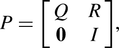
Figure 1 depicts the point-to-game DTMC for when $A$ is serving, with states labeled for reference and modification later on. It has been observed by many, such as Carrari et al. (2017), that states 12 and 16, 14 and 17, and 15 and 18 are equivalent with respect to their transition probabilities. However, our model still treats them as distinct states, as this leaves room for modeling how players mentally approach these points differently when relaxing the identically distributed assumption. “ $A$ Win” and “ $B$ Win” are the only two absorbing states, making the dimensions for the point-to-game DTMC’s $Q$ and $R$ matrices $18 \times 18$ and $18 \times 2$ , respectively. Using the previous DTMC properties, the (1,1)th entry of $W R$ is the probability the model assigns to $A$ winning their service game. The average duration of $A$ ’s service game, in terms of number of points played, is the (1,1)th entry of $W \underline{t_{p}}$ , where $\underline{t_{p}}$ is a vector of 1’s with length 18, effectively summing $W$ ’s first row. We then translate this into time by multiplying by a minutes per point played parameter, $μ$ , estimated using previous data. All output at the point-to-game level, $A$ ’s service game win probability, and the mean duration of $A$ ’s service game, are used as input for the next level (game-to-set) of the model.

Figure 1.

States of the point-to-game DTMC for a single game in a tennis match, with accompanying transition probabilities.

The other levels of the model all closely follow this approach, with a few notable differences. First of all, all other DTMCs require 2 parameters instead of 1 (not counting $μ$ ). This includes tiebreaks which follow an “ $A B B A$ ” serving order. Secondly, Appendix A details a simplification which was taken for the extra points in tiebreaks and advantage sets in the game-to-set level, which both require the player to lead by a margin of 2 to win. Thirdly, absorbing states for the game-to-set DTMC are further expanded to note whether a player wins a set by holding serve or breaking their opponent’s serve. This is for the model to know which player serves first for the next set, though Appendix A shows that for the basic model this distinction is ultimately irrelevant. Lastly, apart from the tiebreak, the vector which we multiplied with the fundamental matrix to estimate durations (i.e., $\underline{t_{p}}$ for the point-to-game level) no longer contains only ones, but rather the corresponding game/set duration estimates of the previous level. Taking the game-to-set level as an example, the entries of its vector, $\underline{t_{g}}$ , alternate between duration estimates for $A$ and $B$ ’s service games, ending in the duration estimate for a tiebreak. Additional time, 1.5 minutes for change of ends breaks and 2 minutes for breaks between sets, is added on to elements of $\underline{t_{g}}$ and $\underline{t_{s}}$ (the corresponding vector for the set-to-match level), respectively, when applicable. This additional time is already in minutes, so $μ$ should be applied to game duration estimates before they are used at the game-to-set and set-to-match levels.

Data

Data used in this study was taken from the excellent GitHub repositories of Sackmann (n.d.). Three repositories were used. First of all, “tennis_atp” and “tennis_wta” include match outcomes for ATP and WTA matches going back to 1968 and 1920, respectively. Alongside these results, aggregate statistics such as the players’ number of service points won and returning points won for the match are available as well. The “tennis_slam_pointbypoint” repository contains more granular data for each individual point, but only for Grand Slam tournaments dating back to 2011 as the collection was done by IBM and Infosys.

In the following experiments, we use this data for training, validation, and testing. For validation and testing, we chose to restrict the range of the datasets to major tournaments (Grand Slams, tour finals, ATP Masters 1000/WTA 1000/WTA Premier). For validation, testing, and estimation of the parameter $μ$ , matches that ended in retirement, default, or walkovers were removed. Taken together, these choices resulted in 6 training sets, each, on average, containing 8033 match entries and roughly 1.1 million points played. Their corresponding testing sets averaged out to 1409 match entries per set, with validation sets being on a similar scale. In agreement with the point-by-point data going back to 2011, we use 12 years of data in total, from 2011 to 2022. We separate the data into three consecutive 4-year intervals for both the ATP and the WTA, with the first three years within an interval being used for training (and validation for the point-specific method) and the remaining years (i.e., 2014, 2018, 2022) for testing. This choice of a 3-year time horizon for training trades data freshness for volume, and we compared its effect to a shorter 1-year time horizon in our initial experiments, with key results and takeaways included in Appendix B. Only 5 train-test dataset pairings are used for duration prediction, as the WTA 2014 test set does not have enough matches with duration recorded.

Individual Methods

In this section, we overview the three methods in the literature before detailing the two new methods we add to their ranks. Before doing so, we note that though some of the five methods introduce more inputs to the model, none of them make changes to the hierarchical structure of the model nor the state-structure of any of its DTMCs. All changes are ultimately centered around providing better estimates of the service point win probability inputs. How far can changes to only this type of variable take us in terms of accuracy? When the service point win probabilities are taken to be the actual realized service point win proportions of their respective matches, the basic hierarchical model consistently yields accuracies over 90% for the test sets¹. Of course, the service point win proportions of a match whose outcome we aim to predict are unobtainable prior to the match, but this showcases the potential in increasing prediction accuracy gained solely in working towards better $p$ estimates.

The most naive method is simply to take a player’s service point win proportion over their matches in the training set. These estimates can vary depending on time horizon length and whether or not the matches have been filtered for only the surface on which we wish to predict. It has previously been mentioned that our preliminary studies in Appendix B examine the effect of shorter time horizons. The effect of surface-filtering is also examined there. Building off of this basic estimate, Barnett and Clarke (2005) incorporate information on opponent return ability. Their opponent-adjusted formula deducts from a player’s $p$ estimate the difference of their opponent’s return point win probability with the mean return win probability of the field. Denoting return point win probability as $q$ and using players $A$ and $B$ as subscripts, we have for $A$ ’s adjusted $p$ playing against $B$ : ${\hat{p}}_{A} = p_{A} - (q_{B} - \bar{q})$ , where $\bar{q}$ is the return point win probability of the field. This method performed the best in Kovalchik’s testing among point-based methods, and even before then, variations had been adopted in studies such as the low-level point model (examining the even lower rally-to-point level) of Spanias and Knottenbelt (2013) and their 2012 study with Madurska on using common-opponent data. Though identical conceptually, applications of this opponent-adjusted formula can vary in how the return point win probability of the field is derived. For each of our experiments, we took the average $q$ of all the players in that experiment’s training set.

The aforementioned study by Knottenbelt et al. (2012) proposes using common-opponent data to adjust for opponent ability. Training data is restricted to a list of common opponents (CO) that the two players have faced in the given time frame. In their study, win probabilities were obtained with respect to each CO and then aggregated, whereas our approach makes use of all available CO data directly for the estimation of a single value of $p$ . Whether or not to restrict the CO list according to surface-relevance, and if so, when to apply this restriction, results in multiple variations to this method. Our preliminary study (in Appendix B) rigorously tests the comparative effectiveness of these variations, providing statistical evidence for the authors’ conjectures on surface-filtering. Only the best among them, with no degree of surface-filtering, is included in the main study. While the CO method provides a way to include opponent information in the training data itself, the abundance of tennis data makes directly using H2H data an option as well. To the best of our knowledge, this has not been tested in the literature, though it comes at the cost of much smaller coverage.

Apart from using H2H data, the other new method we employ is the point-specific method, an attempt at relaxing the identically distributed part of the model’s iid assumption at the point-to-game level. Sim and Choi (2020) conducted extensive statistical tests examining the validity of the iid assumptions at the point-to-game level, concluding the identically distributed piece of the assumption as invalid. Klaassen and Magnus also concede this in Analyzing Wimbledon (2014), but reason that the deviation from the points being identically distributed is small enough that the iid models are still quite useful in the analysis. Through the point-specific method, we examine whether relaxing the identically distributed assumption yields a substantial increase in accuracy, and if so, what points having their own $p$ estimates benefit prediction most. We start by estimating different $p$ ’s for each of the 18 transient states of the point-to-game DTMC. One additional $p$ estimate will be introduced for tiebreaks. Denoting with subscript $i$ the $p$ estimate corresponding to the $i$ th state (and writing $p_{19}$ for the tiebreak $p$ ), our model now takes pairs of vectors of length 19, $p = (p_{1}, p_{2}, \dots, p_{18}, p_{19})$ , as input instead of simply two $p$ estimates. We make an additional partition to each training set, taking the last year, the one closest to the test set, for validation. The $p$ vectors are initially estimated using the other two years’ point-by-point data. Referring to states with their own $p$ estimates as activated, we then begin deactivating states by replacing these $p$ estimates with the general non-state-specific $p$ (calculated by taking the proportion of the player's serving points won in the two-year point-by-point data). A greedy approach is taken, in that the set of deactivated states begins as an empty set, and at each step we calculate what the accuracy score would be for the validation year if each of the remaining activated states were to be deactivated. The state whose deactivation yields the highest validation accuracy will be added to the set of deactivated states to complete the step. The opposite of this exercise, where we start with all states deactivated and begin activating them under a greedy approach, is performed as well. The $p$ vectors are finally estimated using all three years of point-by-point data, and are applied to the testing set in accordance with the states identified for activation. On the duration estimation side, we use the states identified via outcome prediction, but also test out another set of states identified in a similar manner, but with each step looking to minimize RMSE instead of maximize accuracy in the greedy algorithm.

Ensemble Methods

First of all, we note an ensembling method which Knottenbelt et al. (2012) and Kovalchik (2016) both employ, regarding the opponent-adjusted formula and the CO method. Since the former focuses on the opponent’s return ability relative to the field (which is not match-up specific), there is room to combine it with the latter, which aims to use match-up specific information in an indirect way.

A similar application of the opponent-adjusted formula to H2H data does not make as much sense, as the H2H data should already have adjusted for the players’ return ability against the field, as well as how they match up against their opponent. Following from this, we expect the H2H results to be highest in quality (though this may not be the case in practice), followed by the other methods and lastly by the basic estimation. Therefore, our second ensemble method is to prioritize H2H results when a matchup has H2H data, another method’s results if they do not, and use basic estimation for the rest when no other methods apply. We refer to this as the overlay method, since it essentially layers results on top of each other. Furthermore, note that the bottom layer is either from basic estimation or the opponent-adjusted formula, since both have the same coverage (and same imputation method of using field averages). The overlays directly use the model’s binary predictions, but these predictions are taken from the win probabilities the model actually yields. To make use of these probabilities, our next ensemble model makes predictions based on the mean win probabilities of its components. We refer to this third ensemble method as merging.

Taking note that, especially in the context of sports betting, not making a prediction is a valid choice, we also propose two ensemble methods with incomplete coverage of the test matches, much like the CO and H2H methods. The first is a consensus model, which only makes a prediction if all its components are in agreement. The second is a relaxation of the first, needing only a majority to make a prediction.

Finally, on the side of match duration prediction, we also attempt preliminary ensembling. The overlay, consensus, and prediction methods are no longer applicable as they work with binary results, but an ensemble model taking the mean time of its components is examined. For both this model and the aforementioned merging model, there is room for improvement in examining weight distribution beyond a uniform one, but we deem this too large in scope for this particular study.

Results and Discussion

Outcome Prediction

Table 1 presents the experimental results for the individual methods, while Table 2 presents selected results for each ensemble method. In addition to the CO and H2H abbreviations which both tables continue to use, “Basic” refers to the basic results of the point-based hierarchical model, “OAF” refers to the opponent-adjusted formula of Barnett and Clarke (2005), and “PSU” and “PSD” refer to the point-specific method results with one state activated and all-but-one state activated, respectively. (“U” is for “up”, the direction we define where the greedy algorithm starts with no states activated and activates states one-by-one. The reasoning is the plateau shapes which can be seen in Figure 2. “D”, similarly, stands for “down”, using the algorithm that deactivates instead.) “CO(OAF)” refers to the method of applying the opponent-adjusted formula to common opponent data. Furthermore, we use the following notation to differentiate the remaining ensembles. The ensemble’s components are included in its name, with order only making a difference in the overlays – methods that come before being overlaid on ones that come after. Ensembles with “/” connecting its components are overlays, “+” is used for merges, “&” for majorities, and “&&” for consensus.

Figure 2.

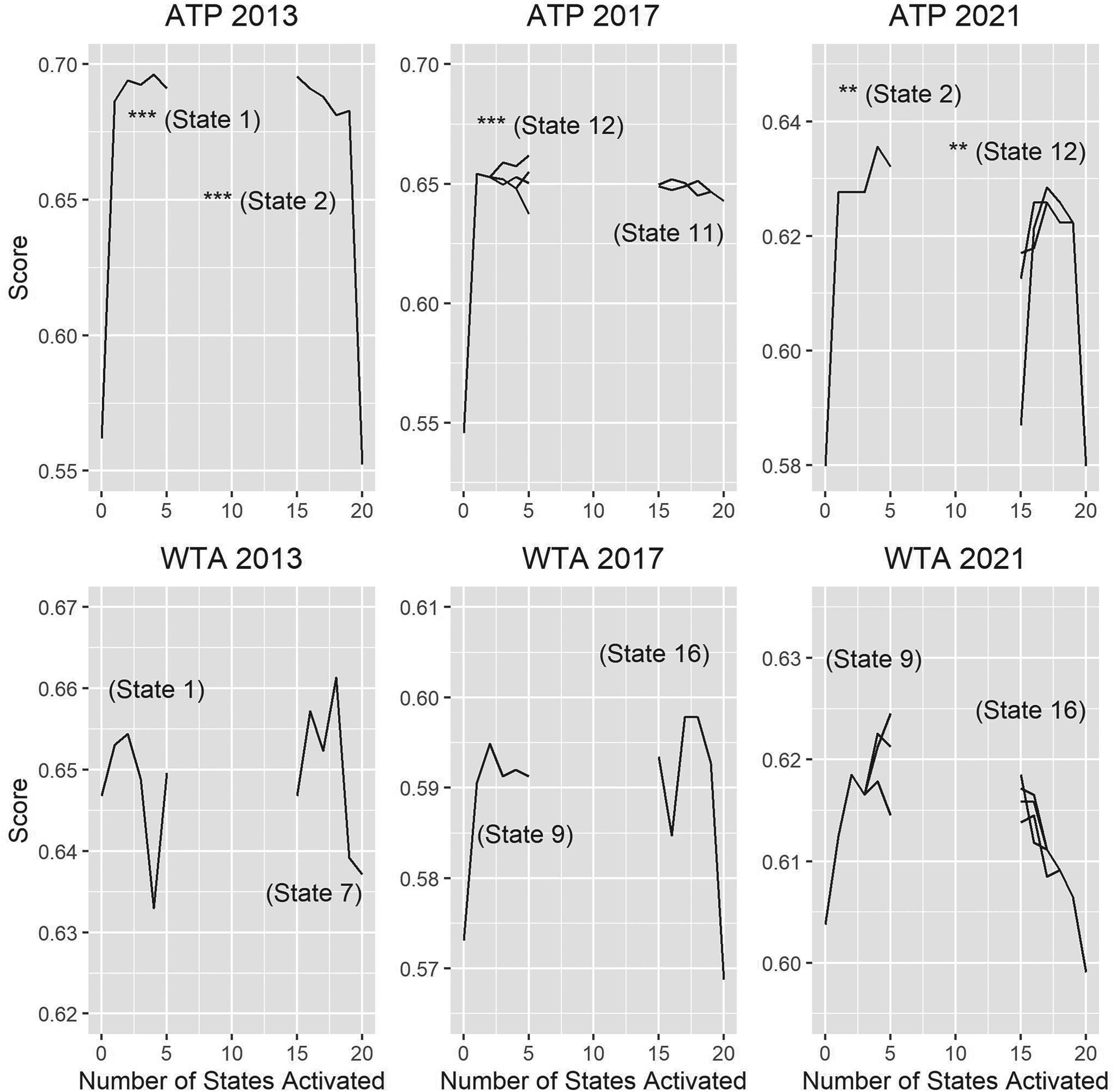
Accuracy score plots corresponding to activations and deactivations of states in the point-to-game DTMC. The first states identified for activation/deactivation are annotated in the plot, along with an indicator for the significance of the jump the activation/deactivation yields (‘***’ - p<0.01, ‘**’ - 0.01<p<0.05, ‘*’ - 0.05<p<0.1, ‘-’ - p>0.95).

Table 1.

Outcome prediction accuracy for individual methods.

	ATP 2014	WTA 2014	ATP 2018	WTA 2018	ATP 2022	WTA 2022
	$(N = 1330)$	$(N = 1467)$	$(N = 1304)$	$(N = 1457)$	$(N = 1220)$	$(N = 1371)$	Mean	Variance
Basic	62.722 (85)	61.283 (95)	62.626 (91)	59.818 (98)	61.386 (91)	59.610 (97)	61.241	0.00018
OAF	68.416^*** (85)	66.258^*** (95)	63.957 (91)	63.006* (98)	65.164 $^{* *}$ (91)	63.166* (97)	64.987	0.00046
CO	63.415 (80)	61.844 (91)	63.395 (84)	58.138 (94)	61.471 (85)	59.055 (93)	61.220	0.00048
H2H	64.340 (40)	62.687 (41)	64.122 (40)	59.070 (44)	61.674 (37)	52.372 $^{-}$ (37)	60.711	0.00204
PSU	57.368 (100)	59.100 (100)	57.669 (100)	57.515 (100)	55.246 (100)	59.227 (100)	57.688	0.00021
PSD	56.992 (100)	58.828 (100)	57.889 (100)	58.270 (100)	55.492 (100)	57.768 (100)	57.542	0.00014

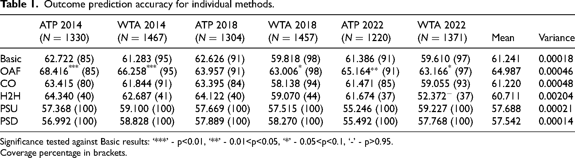
Significance tested against Basic results: ‘***’ - p<0.01, ‘**’ - 0.01<p<0.05, ‘*’ - 0.05<p<0.1, ‘-’ - p>0.95.

Coverage percentage in brackets.

Table 2.

Outcome prediction accuracy for ensemble methods.

	ATP 2014	WTA 2014	ATP 2018	WTA 2018	ATP 2022	WTA 2022
	$(N = 1330)$	$(N = 1467)$	$(N = 1304)$	$(N = 1457)$	$(N = 1220)$	$(N = 1371)$	Mean	Variance
CO(OAF)	$_{* * *} 68.480$ (80)	$_{* *} 64.843$ (91)	$_{* *} 66.606$ (84)	61.290 (94)	63.601 (85)	61.024 (93)	64.206	0.00087
H2H&&CO&&OAF &&CO(OAF)&&PSU	$_{* * }^{ *} 75.338$ (22)	$_{* * }^{ *} 72.188$ (22)	$_{* * }^{ * *} 75.564$ (20)	$_{* }^{} 66.788$ (19)	$_{* * *} 70.046$ (18)	$_{* *} 66.342$ (15)	70.902	0.00163
Consensus of all 6	$_{* * }^{ *} 75.177$ (21)	$_{* * }^{ * *} 72.468$ (22)	$_{* * }^{ * *} 75.581$ (20)	$_{* }^{} 66.917$ (18)	$_{* *} 69.811$ (17)	$_{* *} 66.500$ (15)	70.895	0.00158
H2H&&OAF&&CO(OAF) &&PSU&&PSD	$_{* * }^{ *} 75.241$ (23)	$_{* * }^{ *} 71.667$ (25)	$_{* * }^{ * *} 75.746$ (21)	$_{* *} 66.549$ (19)	$_{* * *} 69.778$ (18)	$_{* *} 66.351$ (15)	70.730	0.00168
CO&&OAF&&CO(OAF)&&PSU	$_{* * }^{ * *} 74.817$ (51)	$_{* * }^{} 68.472$ (57)	$_{* * }^{ * *} 72.103$ (54)	$_{* * }^{} 65.714$ (55)	$_{* * }^{} 69.550$ (47)	$_{* * }^{ *} 67.336$ (54)	69.649	0.00110
CO&&OAF&&CO(OAF)&&PSU&&PSD	$_{* * }^{ * *} 75.841$ (49)	$_{* * }^{} 68.382$ (56)	$_{* * }^{ * *} 72.114$ (51)	$_{* * }^{} 65.580$ (53)	$_{* * }^{} 69.134$ (45)	$_{* * }^{ *} 67.222$ (53)	69.630	0.00137
OAF&&CO(OAF) &&PSU&&PSD	$_{* * }^{ * *} 75.488$ (54)	$_{* * *} 67.791$ (63)	$_{* * }^{ * *} 71.955$ (54)	$_{* * *} 65.271$ (56)	$_{* * *} 68.145$ (50)	$_{* * }^{ *} 66.494$ (56)	69.041	0.00146
CO&&OAF&&CO(OAF)	$_{* * }^{ *} 72.506$ (59)	$_{* * }^{} 68.437$ (67)	$_{* * }^{ * *} 70.655$ (61)	$_{* *} 64.271$ (67)	$_{* * }^{ *} 70.074$ (55)	$_{* * *} 64.853$ (64)	68.696	0.00109
CO&&OAF&&PSU	$_{* * }^{ * *} 73.662$ (53)	$_{* * *} 68.187$ (58)	$_{* * }^{ * *} 71.231$ (55)	$_{* * }^{} 65.581$ (59)	$_{* * }^{} 69.378$ (51)	$_{* * }^{ *} 66.626$ (59)	69.149	0.00090
H2H&&OAF&&PSU	$_{* * }^{ *} 73.988$ (26)	$_{* * }^{ *} 70.284$ (26)	$_{* * }^{ * *} 74.074$ (23)	$_{* }^{} 66.667$ (22)	$_{* * *} 69.685$ (21)	$62.602$ (18)	69.569	0.00195
H2H&OAF&PSU	$_{* * }^{} 71.167$ (78)	$_{* *} 65.566$ (83)	$_{* * }^{ *} 69.224$ (82)	$_{* *} 63.171$ (83)	$_{* * *} 67.606$ (81)	$_{* *} 64.417$ (83)	66.965	0.00092
H2H+CO(OAF)+PSU	$_{* * *} 70.752$ (100)	$_{62.031}^{-}$ (100)	$_{* * }^{ *} 67.868$ (100)	$60.673$ (100)	$_{* *} 65.492$ (100)	61.123 (100)	64.776	0.00167
CO+OAF+CO(OAF)+PSU	$_{63.759}^{-}$ (100)	$_{* *} 64.349$ (100)	63.267 (100)	61.839 (100)	63.852 (100)	$_{*} 62.217$ (100)	63.305	0.00010
H2H+OAF+PSU	$_{63.308}^{-}$ (100)	63.122 (100)	62.883 (100)	61.496 (100)	$_{* *} 65.410$ (100)	61.488 (100)	63.303	0.00021
CO(OAF)/OAF	$_{* * *} 63.383$ (100)	$_{* *} 65.508$ (100)	$_{*} 64.417$ (100)	61.290 (100)	62.951 (100)	61.853 (100)	63.193	0.00025

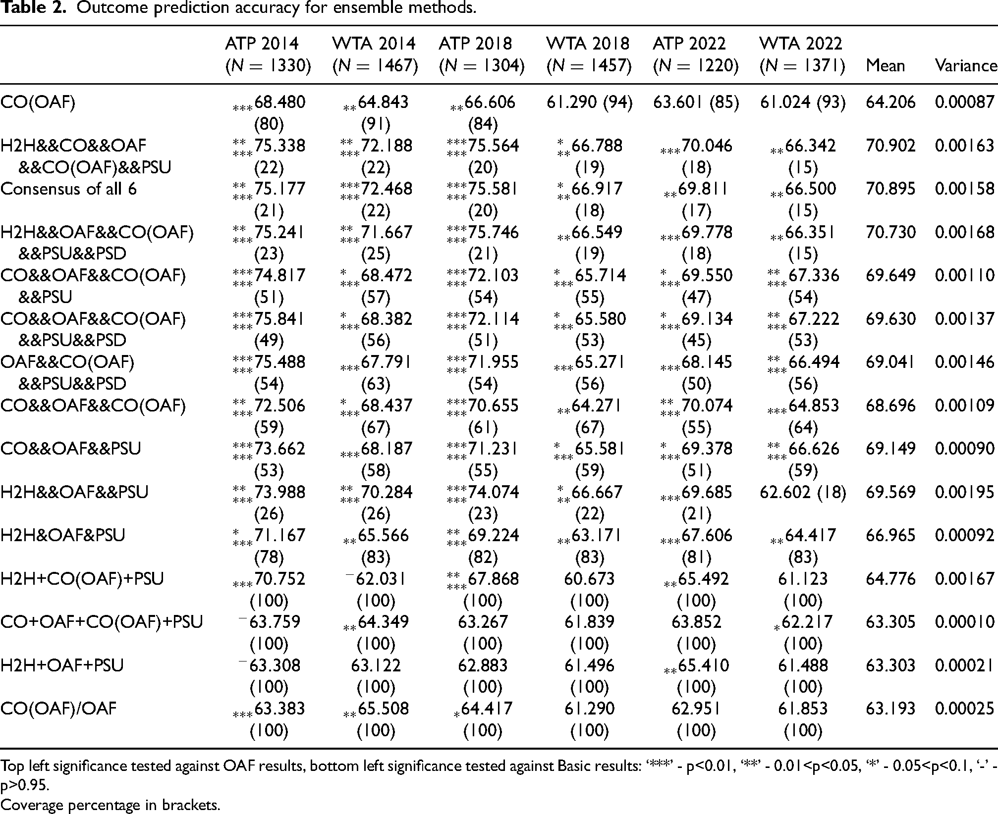
Top left significance tested against OAF results, bottom left significance tested against Basic results: ‘***’ - p<0.01, ‘**’ - 0.01<p<0.05, ‘*’ - 0.05<p<0.1, ‘-’ - p>0.95.

Coverage percentage in brackets.

The tables also include the coverage for each match (i.e., the percentage of matches in the test set for which we have the data necessary to apply a method) in brackets. We can see in Table 1 that the basic model prediction and OAF always share the same coverage, as one player’s service point data is their opponent’s return point data. Even for these two methods which only require service point data, complete coverage is not achievable, with new and improving players continuously being given opportunities in major tournaments. The standard imputation procedure used in previous studies is to use the average service point win probability (and average return point win probability) of the training set. However, taking into account that many of the other methods, in fact, all other methods apart from PSU, PSD, and the overlays, do not have complete coverage, as well as the remark in “Ensemble Methods” on how abstaining from prediction is a valid option in many match prediction contexts, we chose to keep and use the non-imputed Basic and OAF results to make fairer comparisons with the other methods having incomplete coverage. The results with imputation for the Basic and OAF methods were still obtained, with ATP 2014 being the only test set to see a significant (i.e., with p-values of p $=$ 0.0031 and p $=$ 0.009 for Basic and OAF, respectively) decrease in accuracy, falling to 59.023% and 63.835%, respectively. These imputed versions of Basic and OAF results are only used for constructing overlays, which do strive for complete coverage, and testing significance of other methods which have complete coverage. All other methods are tested against the versions of Basic and OAF with incomplete coverage, and all significance values for match outcome prediction accuracy are obtained through two sample z-tests for proportions (Sheskin, 2000).

Individual Methods

Looking first to the methods established in the literature (i.e., Basic, OAF, and CO), Table 1’s results conform with those in the study of Kovalchik (2016) (performed with 2014 data) with regards to OAF being the most accurate. This is consistent throughout the other two testing years for both ATP and WTA, though p-values are most significant for 2014. Across testing sets, OAF yields a 3.58% increase to the basic baseline results while CO yields moderate, but not significant, increases. H2H comes with a considerable drop in coverage, but only performs slightly better than CO on the testing sets apart from WTA 2022, where it is significantly worse than the basic baseline. The exceptionally low accuracy for WTA 2022 weighs heavily on its variance, which is on another order of magnitude compared to that of the other individual methods. (Since all methods are tested on the same six sets, we take the sample variance of the six scores to roughly compare variability between methods.) Overall, the failure of H2H to significantly boost model performance aligns with the conclusions of the preliminary studies on surface-filtering and time horizons in Appendix B, which stressed the importance of quantity over quality of the data when aiming to boost performance through estimating $p$ . In addition to a restrictive sample size, a pure player-specific match-up-focused approach may also be overadjusting to aspects of a specific opponent’s game that is actively (and possibly even deliberately) undergoing change. Due to the often long length of time between H2H matches (and the presence of events such as the COVID-19 pandemic that could possibly constitute change points), it is easy for the data to not reflect recent changes to a player’s playing style that may be decisive. Contrasting this with the other less-specific adjusting methods, OAF and CO indeed leave more room to pick up on recent changes. Though its results are particularly volatile, H2H results in the absence of large amounts of H2H data still have prediction value, as we shall see shortly as they become important components of some of the best ensembles.

This is also the case for the individually unspectacular PSU and PSD results, which are significantly worse than the baseline five times out of twelve. What is worth highlighting first is the plateau phenomenon in Figure 2. More precisely, for all ATP validation sets as well as WTA 2017, there exists a state corresponding to the train-validation dataset pairings, which when activated, yields a significant boost to performance on the validation set. Another state exists for which deactivation yields a similar boost. The way activations and deactivations actually change prediction results is by toggling the model’s perception of how strong a player is. (Note that this perception is not a single value that can be directly compared as in the case of earlier $p$ estimates. $p_{1}, p_{2}, \dots, p_{18}$ are indeed consolidated into the probability of a player winning their service game, $p_{G}$ , which is independent of the opponent. But the tiebreak DTMCs take input from both players’ $p_{19}$ to form the probability of winning a tiebreak $p_{T}$ . How $p_{T}$ is weighed into the final match prediction is decided by the probability of a set going to tiebreak, which also takes input from both players’ $p_{G}$ . So opponent-adjusting is happening for this model to a certain extent, and we refer to the model’s perception of a player in a fuzzier sense.) Under our greedy approach, the training set provides the point-based tendencies of the players observed for the training set’s time period, and the validation set plays the role of a filter, highlighting tendencies of certain players that persist into the validation set’s time period for activations, and tendencies that have ceased for deactivations. The forming of plateaus indicate players do have point tendencies that can be exploited for prediction, but states identified are only those best suited for increasing the accuracy on the validation set as a whole and not for specific groups of players. Therefore, there is room for more consistent identification of states if training and validation is done only for individuals or groups of players that share certain point tendencies. This is a considerable challenge, as it would be placing an even tighter restriction on the amount of data available, an amount already smaller than other methods due to the need for point-by-point data. Another area of potential improvement which hampers current performance is the large time gap between the training, validation, and testing datasets, especially since professional tennis players are regularly working to address their point tendencies.

Ensemble Methods

With OAF as the uncontested standout of the individual methods, it makes sense for it to serve as the benchmark of the ensemble methods, with all significance markers to the top-left of the scores in Table 2 calculated with respect to OAF results. (As noted before in “Individual Methods”, only the overlays are compared to the imputed OAF results.) In view of this, we see that CO(OAF) does not provide a significant boost overall. Though for ATP 2018, CO(OAF) significantly increases accuracy of the basic model while OAF does not, this boost builds on OAF’s incremental boost and is ultimately still not significant enough when calculating significance with respect to OAF.

We finally arrive at the set of models that yield the most promising results, which are the consensus models. The first three ensembles after CO(OAF) in Table 2 are the top three consensus models in terms of accuracy averaged over the six testing sets. All three contain at least five components, and consequently have quite low coverage all hovering around 20%. The relationship between coverage and accuracy is more completely illustrated in Figure 3a, which plots coverage against accuracy for all 57 consensus models. The regression line has a significant negative slope (p = $9.7 \times 10^{- 6}$ ), signaling an overall trade-off between coverage and accuracy. However, the linear fit is evidently a poor one, and even around 60% coverage, we can find consensus models with accuracy near 70%. This is even more the case with the fit for coverage and average significance in Figure 3b, with a significant positive slope (p $=$ 0.023) but an even poorer linear fit which leaves room for models with over 50% coverage and very competitive significance scores. Interestingly, none of the top three consensus models for accuracy have the best average significance scores, which also belong to the cluster of models in the center of Figure 3a. We can see in Table 2 that this is because none of the three models are significant for WTA 2022, which points to H2H’s interference. Indeed, the next three consensus models in Table 2 are the first three with H2H removed, and the first of these three has the most significant consensus model on average with a p-value of 0.039. We can see H2H’s positive effect here on pure accuracy, as well as its volatility in WTA 2022 seep through. PSU’s value is also on display when we compare the decreases that were to happen to accuracy and significance when PSU and CO(OAF) are removed, respectively, from the most significant model. In both aspects, PSU has a larger effect than CO(OAF).

Figure 3.

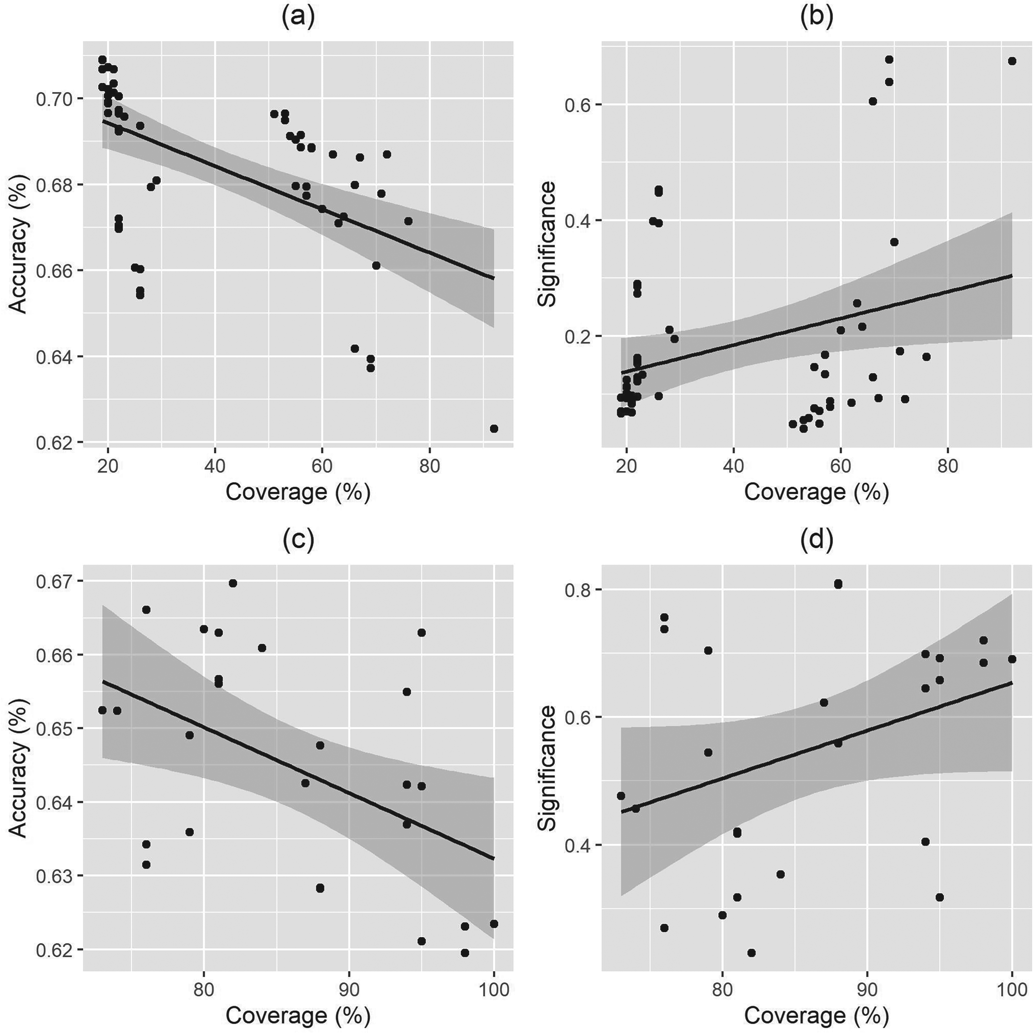
Ensemble coverage against average accuracy and significance for consensus (a, b) and majority (c, d) models.

The majority model highlighted in Table 2 is the top majority model in both accuracy and significance. We cannot conclude definitively that H2H’s boost to accuracy for the majority models does not come with as considerable a reduction to WTA 2022 significance as it did with the consensus models. But this negative effect is evidently dampened, with H2H&OAF&PSU yielding by far the most significant increase for WTA 2022 (p $=$ 0.007 against Basic, p $=$ 0.208 against OAF) among the majority models². When compared to its consensus counterpart with the exact same components, the majority model still loses out in accuracy and significance, but has a much broader coverage, justifying its use if coverage cannot fall below a certain rate. More broadly, when we construct the same plots for the majority models as was done for the consensus models, we see in Figures 3c and 3d the same overall trade-offs between coverage and accuracy/significance, but with an even weaker, noisier relationship, and with respect to a narrower, higher range of coverages.

Table 2 also highlights the best merge model (first in accuracy, second in significance) and the best overlay model (first in accuracy and significance), as well as the merge counterparts to the most significant models identified above. Comparing counterpart performances for the merge models and the lack of significance for the overlay model, we conclude that these latter two methods do not boost performance the way the consensus and majority methods do. This may have been expected for the overlays as soon as the H2H individual results did not outperform OAF, but for the merge method, problems may lie with the equal weights the method assigns to all components that have coverage for a match.

Duration Prediction

All RMSE results from the duration prediction of individual methods are presented in Table 3, along with CO(OAF) and the best mean prediction model (lowest average RMSE, second smallest significance value). Significance was derived using two-sample t-tests (Sheskin, 2000) compared to the basic model results³. Unlike in outcome prediction, the applications for duration prediction do not allow the picking and choosing of matches to predict. So, standard imputation is used for both Basic and OAF. We can see duration prediction performance shares some characteristics with outcome prediction results (e.g., relatively strong ATP 2014 performance, relatively strong OAF performance, high variance for H2H, CO(OAF) on par with OAF with no clear improvement). This relationship will be explored further in the next section. Overall, the ability of the point-based hierarchical model to predict match duration seems limited regardless of method. Additionally, not reflected in Table 3 is a clear tendency for all methods apart from H2H to overestimate match duration on average.

Table 3.

Duration prediction RMSE.

	ATP 2014	WTA 2018	ATP 2018	WTA 2022	ATP 2022
	$(N = 1330)$	$(N = 1457)$	$(N = 1304)$	$(N = 1371)$	$(N = 1220)$	Mean	Variance
Basic	42.833 $^{* *}$ (85)	49.374 (98)	43.185 (91)	33.012 (97)	45.134 (91)	42.707	36.146
OAF	40.927 (85)	49.094 (98)	42.713 (91)	33.075 (97)	44.656 (91)	42.093	34.666
CO	42.176 (80)	50.289 (94)	43.561 (84)	32.773 (93)	44.835 (85)	42.727	40.428
H2H	40.738* (40)	64.902 (44)	46.788 $^{-}$ (40)	34.190 (37)	46.229 (37)	46.569	130.882
PSU.A	42.072 (100)	49.235 (100)	42.949 (100)	33.224 (100)	45.116 (100)	42.519	34.661
PSD.A	40.957 $^{* *}$ (100)	49.148 (100)	42.576 (100)	33.082 (100)	44.406 (100)	42.034	34.454
PSU.E	41.981 (100)	49.186 (100)	42.743 (100)	33.120 (100)	44.935 (100)	42.393	34.723
PSD.E	40.952 $^{* *}$ (100)	49.148 (100)	42.508 (100)	33.046 (100)	44.371 (100)	42.005	34.563
CO(OAF)	40.775 (80)	50.090 (94)	43.042 (84)	33.438 (93)	44.149 (85)	42.299	36.381
H2H+OAF+ CO(OAF)+PSD.E	39.812^*** (100)	48.663 (100)	41.862 (100)	32.471 (100)	43.728 (100)	41.307	35.149

Significance tested against Basic results: ‘***’ - p<0.01, ‘**’ - 0.01<p<0.05, ‘*’ - 0.05<p<0.1, ‘-’ - p>0.95.

Coverage percentage in brackets.

For point-specific results, those ending in “A” use the states identified in prior experiments where the greedy algorithm aims to increase outcome prediction accuracy. Those ending in “E” instead have the algorithm choosing the lowest RMSE at every step. The states identified for each experiment are different between the two approaches, apart from WTA 2017 which sees state 16 deactivated for both. Unlike when selecting for accuracy, selecting for lower error fails to yield a valley shape that would correspond to the plateau phenomenon. The lack of valleys is not completely surprising, as the activation of states toggle relative strengths of players, which has a much more direct relationship with match outcome than match duration. That is not to say there is no relationship. Though roughly the same, all “E” RMSE scores are bounded above by their corresponding “A” scores, giving some evidence that the targeting at least has some effect. Perhaps surprisingly, point-specific results are on par with OAF, with PSD.E often even slightly better. The mean duration models are similar in that they make consistent improvements which ultimately remain insignificant. When focusing only on RMSE, all 247 mean duration models improve on the baseline, decreasing the mean RMSE over the five test sets by 2.27% on average, with H2H+OAF+CO(OAF)+PSD.E leading with 3.27%. In view of the potential for improvements in these preliminary point-specific (more data, targeting specific groups, and closer times between train/validation/test) and mean duration methods (moving beyond uniform weights), these two techniques make for promising leads when exploring further match duration prediction with point-based hierarchical models.

Comparison of Outcome and Duration Prediction Results

In this section, we overview some results from the previous two sections with a focus on the joint performance of the various point-based Markov models on both outcome and duration prediction. Table 4 is a representative summary of performance metrics averaged across all five datasets (recall that WTA 2014 data is not available for duration prediction). Table 4’s last two entries, specifying ensemble components, refer to the best performing ensembling methods for each respective prediction problem. These are consensus ensembling methods for outcome prediction and, by default, the mean duration models for duration prediction. Additionally, since PSU.E and PSD.E results are superior to PSU.A and PSD.A results for duration prediction, all models involving PSD in Table 4’s comparisons refer to PSD.E on the duration prediction side. We can see the effect of individual methods are more pronounced for outcome prediction. Similarly, the impact of ensembling is positive for both areas, but we do not see a drop in RMSE commensurate with the jump in outcome prediction accuracy. Nevertheless, higher outcome prediction accuracy does seem to be associated with slightly lower RMSE values at large in the experimental results. This is the case not only when mean duration results are compared against consensus ensembling, but also majority and merge ensembling as well. Looking back to the individual models, this is not as clear, especially in Table 4’s high level summary. CO slightly raises both accuracy and RMSE, H2H only slightly increases accuracy but drastically increases RMSE, and PSD is not good for accuracy but surprisingly, relatively decent for RMSE.

Table 4.

Comparison of outcome and duration prediction results for select models.

	Outcome Prediction Accuracy	Duration Prediction RMSE
Basic	60.651	42.707
OAF	64.231	42.093
CO	61.220	42.727
H2H	60.711	46.569
PSD	57.542	42.005
Ensemble of CO, OAF, CO(OAF), PSD	69.492	41.550
Ensemble of H2H, OAF, CO(OAF), PSD	70.347	41.307

This last overall point, on how correlated the outcome and duration performances of the various models are, warrants more systematic and rigorous exploration. To this end, we first normalize all prediction results with respect to their datasets of origin. More specifically, for both accuracy and RMSE, we deduct the mean of the metric over all experimental results from its dataset, and then divide by the standard deviation over the same set of results. This is to account for baseline differences between the datasets, most notably WTA 2022, where the RMSE scores are in the low-thirties rather than the low-fourties like the other four datasets, and the accuracy score under the Basic model is the only one to be under 60%. After normalization, we measure for negative correlation using both Pearson correlation which captures linear association, as well as Kendall’s Tau, which measures ordinal association (Sheskin, 2000). Because of how aligned PSU and PSD results are, only PSD (PSD.E for duration) is used for these correlation calculations to avoid inflating the point-specific method’s influence.

Taken together, or on their own (though this only uses 5 data points per model), the individual methods do not have significant, or even always negative, correlation.⁴ On the other hand, the Pearson correlation for mean duration models with consensus ensembling is $- 0.4968657$ , which is significant with a p-value less than $1 \times 10^{- 15}$ . Kendall’s Tau is similar, $- 0.3096162$ with a significance level under $1 \times 10^{- 14}$ . Correlation between mean duration results and majority ensembles is also negative for both correlation measures. The significance level drops to less than $1 \times 10^{- 5}$ for both, which is still extremely significant. Merge ensembles only have slight negative correlation with mean duration models, and the corresponding p-values, while small, are not low enough to be deemed significant. Altogether, we have ample evidence to conclude a strong negative correlation between the results of the recommended ensemble methods for outcome and duration prediction (the merge ensembles were not strong to begin with and are not considered recommended ensembling models). Equivalently, we have strong positive correlation between outcome and duration prediction performance for the recommended ensemble methods.

Concluding Remarks

Among the experimental results, the consensus models for predicting match outcome are far superior to other models, boosting the accuracy of the point-based approach to be competitive with models using machine learning techniques. In comparison with their consensus counterparts, majority models trade accuracy for coverage, but remain competitive with opponent-adjusted models, which our studies reaffirm to lead prior existing methods in performance. Beyond the implications of these results to anyone looking to speculate on tennis match outcomes, the results add to the literature demonstrating the potential of ensembling methods for researchers in sports analytics and predictive analytics, at large. The positive effects of ensembling are apparent for duration prediction as well, with even rudimentary mean duration models consistently lowering prediction RMSE. More generally, this paper systematically applied variations on the point-based hierarchical Markov model to predicting match duration, finding a tendency to overestimate and identifying the opponent-adjusted formula and point-specific modifications to offer improvements among individual methods. Point-specific modifications play important roles in consensus and majority ensembles, and uncover potential for more predictive power, potential which is partially captured in the plateau phenomenon on the accuracy side (though, perhaps counterintuitively, it is the duration side with better individual performance). Their performance is dampened by their requirements for data higher in volume and denser in time. The same goes for using H2H data, as well as other modifications we attempted which did not yield notable results: decaying service point win probabilities to account for stamina, additional states to capture momentum swings, player-specific (or player-profile-specific) input, and specific return point win probabilities for break points in conjunction with the opponent-adjusted formula.

Further work can be done to build on the strength of the consensus models. More point-based models can be included, such as the low-level point model of Spanias and Knottenbelt (2013) and the Bayesian hierarchical model of Ingram (2019), but the net can be cast even wider to include models which use regression, NNs, etc. While the intuition for consensus models is clear, more interpretability into why they perform so well (while majority models comparatively do not) would be helpful. As for other ensembles, both the merges and the mean duration models aggregate predictions using uniform weights, which after further tuning may yield interesting results. As mentioned in the previous paragraph, as well as “Results and Discussion”, point-specific methods show promise, but would have more to offer if more point-by-point data outside of Grand Slam tournaments were available to target specific players or playing styles closer to the time of prediction. An increase in the amount of point-by-point data would also enable an investigation of relaxing the independence of points assumption for the point-based model (whereas our point-specific model only relaxes the identically distributed assumption). Finally, because of the transparency of the point-based hierarchical Markov models, any method applied for pre-match prediction can just as easily be used for in-match prediction as well, with the only difference being to change the initial state of the DTMCs from 0-0 (at the game, set, and match levels) to reflect the current stage of the match.

Footnotes

Acknowledgments

We would like to thank the anonymous referees and Editor for their helpful comments and suggestions, which have narrowed the focus and improved the presentation of this paper. Thank you to Jeff Sackmann for amassing, maintaining, and sharing the datasets used for this study. We would also like to acknowledge Stephanie Kovalchik for answering our queries on her 2016 study.

ORCID iDs

Chengzhi Wang

Steve Drekic

Funding Statement

The author(s) disclosed receipt of the following financial support for the research, authorship, and/or publication of this article: Natural Sciences and Engineering Research Council of Canada through its Discovery Grants program [RGPIN-2016-03685].

Declaration of Conflicting Interest

The authors declare no potential conflicts of interest with respect to the research, authorship, and/or publication of this article.

Notes

Appendices

References

Achlak

(2018) A Markov chain model for serve and rally competitions. Master's diss., University of Waterloo.

Adler

Ross

(2012) Score probabilities for serve and rally competitions. Mathematical Scientist 37(1): 47–54.

Barnett

(2016) A recursive approach to modeling the amount of time played in a tennis match. Journal of Medicine and Science in Tennis 21(2): 27–35.

Barnett

Clarke

(2005) Combining player statistics to predict outcomes of tennis matches. IMA Journal of Management Mathematics 16(2): 113–120.

Buhamra

Groll

Brunner

(2024) Modeling and prediction of tennis matches at grand slam tournaments. Journal of Sports Analytics 10(1): 17–33.

Buhamra

Groll

Gerharz

(2025) Comparing modern machine learning approaches and different forecast strategies on grand slam tennis tournaments. Journal of Sports Analytics 11: 1–18.

Carrari

Ferrante

Fonseca

(2017) A new Markovian model for tennis matches. Electronic Journal of Applied Statistical Analysis 10(3): 1–35.

Clarke

Dyte

(2000) Using official ratings to simulate major tennis tournaments. International Transactions in Operational Research 7(6): 585–594.

Duen

Peker

(2024) Predicting the duration of professional tennis matches using MLR, CART, SVR and ANN techniques. In: Intelligent and fuzzy systems, intelligent industrial informatics and efficient networks proceedings of the INFUS 2024 Conference, Vol. 1, pp.332–340.

10.

Grinstead

Snell

(1997) Introduction to Probability. 2nd Revised Ed. Providence: American Mathematical Society.

11.

Gupta

Assaf

(2024) Tennis match outcome prediction using machine learning and in-match statistics. In: IEEE MIT Undergraduate research technology conference proceedings.

12.

Ingram

(2019) A point-based Bayesian hierarchical model to predict the outcome of tennis matches. Journal of Quantitative Analysis in Sports 15(4): 313–325.

13.

Jhawar

(2022) Predicting tennis match outcomes. In: 2022 International conference on futuristic technologies proceedings.

14.

Klaassen

Magnus

(2014) Analyzing Wimbledon: The Power of Statistics. Oxford: Oxford University Press.

15.

Knottenbelt

Spanias

Madurska

(2012) A common-opponent stochastic model for predicting the outcome of professional tennis matches. Computer and Mathematics with Applications 64(12): 3820–3827.

16.

Kovalchik

(2016) Searching for the GOAT of tennis win prediction. Journal of Quantitative Analysis in Sports 12(3): 127–138.

17.

Kovalchik

Ingram

(2018) Estimating the duration of professional tennis matches for varying formats. Journal of Quantitative Analysis in Sports 14(1): 13–23.

18.

Leitner

Zeileis

Hornik

(2009) Is federer stronger in a tournament without nadal? An evaluation of odds and seedings for wimbledon 2009. Austrian Journal of Statistics 38(4): 277–286.

19.

Lisi

Grigoletto

(2021) Modeling and simulating durations of men’s professional tennis matches by resampling match features. Journal of Sports Analytics 7(2): 57–75.

20.

Newton

Keller

(2005) Probability of winning at tennis i. theory and data. Studies in Applied Mathematics 114: 241–269.

21.

O’Donoghue

Simmonds

(2019) Probability of winning and match length in tiebreak ten tennis. International Journal of Performance Analysis in Sport 19(3): 402–416.

22.

Sackmann

(n.d.) Tennis data, available at: https://github.com/JeffSackmann (accessed 22 September 2024).

23.

Schutz

(1970) A mathematical model for evaluating scoring systems with specific reference to tennis. Research Quarterly. American Association for Health, Physical Education and Recreation 41(4): 552–561.

24.

Sheskin

(2000) Handbook of Parametric and Nonparametric Statistical Procedures (2nd Edition). London: Chapman & Hall.

25.

Sim

Choi

(2020) The winning probabilities of a game and the importance of points in tennis matches. Research Quarterly for Excercise and Sport 91(3): 361–372.

26.

Somboonphokkaphan

Phimoltares

Lursinsap

(2009) Tennis winner prediction based on time-series history with neural modeling. In: Proceedings of the international multiconference of engineers and computer scientists, Hong Kong.

27.

Spanias

Knottenbelt

(2013) Predicting the outcome of tennis matches using a low-level point model. IMA Journal of Management Mathematics 24(3): 311–320.

28.

Sten-Ziemons

(2024) US Open and the controversy over night sessions. DW News, available at https://www.dw.com/en/us-open-and-the-controversy-over-night-sessions/a-70121878 (accessed 30 September 2024).

29.

Wilkens

(2021) Sports prediction and betting models in the machine learning age: The case of tennis. Journal of Sports Analytics 7(2): 99–117.

30.

Yue

Chou

Hsieh

M-H

, et al. (2022) A study of forecasting tennis matches via the glicko model. PloS one 17(4): e0266838.

Boosting markovian tennis prediction: Ensembling and point-specific methods for match outcome and duration

Abstract

Keywords

Introduction

Literature Review

Methods

Hierarchical IID Model

Data

Individual Methods

Ensemble Methods

Results and Discussion

Outcome Prediction

Individual Methods

Ensemble Methods

Duration Prediction

Comparison of Outcome and Duration Prediction Results

Concluding Remarks

Footnotes

Acknowledgments

ORCID iDs

Funding Statement

Declaration of Conflicting Interest

Notes

Appendices

References