Sage Journals: Discover world-class research

Abstract

In this article, different modern machine learning and regression approaches for modeling and prediction of tennis matches in Grand Slam tournaments are investigated. Our data include information on 5013 matches in men's ssGrand Slam tournaments from the period 2011 to 2022. The investigated methods focus on modeling the probability of the first-named player to win the respective match. Moreover, different features are considered including the players' age, the ATP ranking and points, bookmakers' odds, Elo rating, and two additional age variables, which take into account the optimal age of a tennis player. We compare the different regression approaches to modern machine learning approaches with respect to various performance measures. Moreover, we also investigate different forecast strategies. First of all, a cross-validation-type strategy for all matches between 2011 and 2021. We also use an “expanding window” strategy by continuously updating the training data to analyze the predictive performance of the approaches on the tournaments from 2022. Finally, a “rolling window” strategy is used with only 3 years of tournaments as training data. We then select small subsets of best models with largest average ranks and investigate those in more detail by the help of interpretable machine learning techniques.

Keywords

Grand Slam tournaments tennis matches machine learning prediction model selection cross validation rolling window

Introduction

Recently, various statistical and machine learning methods for modelling both tennis matches and whole tournaments have been introduced, leading to an expansion of existing techniques for predicting match-winning probabilities in tennis. Consequently, once all individual matches can be predicted, it may also be possible to calculate the winning probabilities for an entire tournament.

In recent years, machine learning (ML) models were employed to forecast the winners of tennis matches. Somboonphokkaphan et al. (2009) introduced an approach that is able to predict match winners by utilizing both match statistics and environmental data, which uses a Multi-Layer Perceptron (MLP) in combination with a back-propagation learning algorithm. MLP is a fundamental type of Artificial Neural Network (ANN), which are an effective method for addressing real-world classification task and are especially useful for predicting outcomes when they have access to extensive databases and can handle incomplete or noisy data. Whiteside et al. (2017), developed an automated stroke classification system in order to quantify the hitting load in tennis using machine learning models such as a cubic kernel support vector machine. Wilkens (2021) builds on prior research by exploring various ML techniques, including neural networks and random forests, using one of the largest datasets for professional men’s and women’s tennis matches. He found that the average prediction accuracy cannot exceed approximately 70%.

In Sipko and Knottenbelt (2015), the authors predicted the winner of the tennis match based on the probability of serve points won which in turn gives the probability of a player winning the match. They define a method of extracting 22 features from raw historical data, including abstract features, such as player fatigue and injury. Then, by using the resulting data set, they developed and optimized models which were able to outperform Knottenbelt’s Common-Opponent model based on machine learning algorithms such as artificial neural networking. The authors believe that machine learning can bring new innovation in tennis betting as the neural networking generates a 4.35% return on investment in the betting market, which is an improvement of about 75% over the current state-of-the-art stochastic models. Furthermore, Gao and Kowalczyk (2021) constructed a model that predicts tennis match outcomes with high accuracy over 80%, much larger than predictions using betting odds alone, and identified serve strength as a key predictor of match outcome. This was done by using a random forest classifier that highlights the importance and relevance of simple models in the age of deep learning. Moreover, a wide variety of features to capture information about physical, psychological, court-related, and match-related variables are included in a large data set of tennis matches, which is compiled and processed from ATP data from 2000 to 2016. Finally, an overview of modelling and predicting tennis matches at Grand Slam tournaments by different regression approaches has been presented in Buhamra et al. (2024).

In the present work, we focus on several ML modelling approaches, which are applied on tennis Grand Slam tournament match data. Additionally, we proceed further with the comparison of those approaches to the regression models investigated in our previous work (see Buhamra et al., 2024). To achieve this, we use the same data analyzed in Buhamra et al. (2024), which was created from the deuce R package (Kovalchik, 2019), and includes information on 5,013 matches from men’s Grand Slam tournaments between 2011 and 2022. Several features are available, such as the players’ age, ATP ranking and points, odds, Elo rating, and two other age-based variables that account for the “optimal” player’s age, which was found to be in the interval of $[28; 32]$ years (Weston, 2014). Various machine learning and regression approaches will be introduced that are then compared via different performance measures. Moreover, as it is a generally known result that feature engineering often also is quite a crucial aspect for the modeller (and sometimes even more relevant than the choice among different types of statistical or machine learning models), we analyze the impact of different types of forecasting strategies: a cross-validation-type strategy for all matches between 2011 and 2021, an “expanding window” strategy by continuously extending the training data, and a “rolling window” strategy based on only three years of tournaments as training data.

The rest of the article is structured as follows. Section “Data” briefly introduces the data set and defines the objectives of this work. Then, in Section “Statistical and machine learning methods”, different machine learning modelling approaches are introduced, including classification trees, random forest, XGBoost, support vector machine (SVM) and artificial neural networks (ANNs). Besides, some classical regression modelling approaches and corresponding regularization concepts such as the Least Absolute Shrinkage and Selection Operator (LASSO) and non-parametric spline techniques are defined. More details on the regression models and a benchmark model are introduced in Section “Further modelling details and evaluation aspects”. Moreover, three performance measure are defined and two approaches from the field of interpretable machine learning (IML) are described, which are then used to interpret the best machine learning model. In Section “Results”, all modelling approaches are compared via the different forecasting strategies and the introduced performance measures, on the one hand on all Grand Slam tournaments from 2011 to 2021 via a leave-one-tournament-out CV-type strategy. On the other hand, we employ an expanding window approach on the Grand Slam tournament 2022, as well as a rolling window approach with only three years of tournaments as training data in order to have very recent prediction results. Finally, Section “Summary and overview” summarizes the main results and concludes.

Data

In this section, we shortly introduce the data set from Buhamra et al. (2024), which was compiled based on the R package deuce (Kovalchik, 2019). It contains the following information for 5,013 matches in men’s Grand Slam tournaments from 2011 to 2022:

Player1: name of (randomly chosen) first-named player.

Player2: name of (randomly chosen) second-named player.

Year: year when the match took place (ranging from 2011 to 2022).

Tournament: Grand Slam tournament where the respective match took place (Australian Open, French Open, Wimbledon, US Open).

Surface: factor variable describing the surface on which the match was played (“hard”,“clay” or “grass”).

Victory: binary target, determining whether the first-named player won the match (1: yes, 0: no).

Age: metric predictor capturing the age difference of the players (in years); age of the 2nd player was subtracted from that of 1st player.

Prob: difference in winning probabilities of both players, obtained from their average odds (see AvgProb1 and AvgProb2 below); winning probability of 2nd player is subtracted from that of 1st player.

Rank: difference in players’ rankings, calculated by subtracting the rank of 2nd player from that of 1st player. For this, the rank of the players at the start of the tournament is used. The position in the ranking is determined by the ATP points.

Points: difference in ATP points; points of 2nd player are subtracted from those of 1st player; points are awarded for each match won per tournament. Wins in later rounds of a tournament are valued higher than wins in the first rounds of a tournament. Points expire after 52 weeks. Again, the players’ points at the start of the tournament are used.

Elo: difference in Elo rating; Elo rating of 2nd player is subtracted from that of 1st player; Elo rating takes into account whether a player played against a higher or lower ranked player. It increases more if a player wins against a player with a large Elo rating than if he wins against a player with a lower one; it is updated after each new match of a player.

Age.30: first, the distance between the age of the players and reference age of 30 years is calculated, then the corresponding difference between both competing players is calculated, as e.g. for Age. This is because the standard Age variable from above does not contain enough information. For example, a 25-year-old player typically has an advantage over a 20-year-old one, while a 40-year-old player typically has a disadvantage over a 35-year-old one. However, in both cases, the age difference is 5 years. Following Weston (2014), who argued that the optimal age of tennis players is within $[28; 32]$ years, we use 30 years as the mid point of the interval as reference age.

Age.int: first, the distance to the closer limit of the interval was used, i.e. for players younger than 28 the distance to 28 was calculated, while for players older than 32 the distance to 32 was computed. For players with an age within $[28; 32]$ years the distance was set to 0. Then, the difference between both players was calculated.

AvgProb1: average winning probability of Player 1, based on the average odds from several different betting providers, which are provided in the deuce package (obtained from https://www.oddsportal.com/).

AvgProb2: Same as AvgProb1, but from the perspective of Player 2. Note that per match we have AvgProb1 + AvgProb2=1.

B365.1 Winning odds for Player 1 obtained from the specific bookmaker Bet365. Exemplarily, winning odds of 2.31 for Player 1 yield a return of 2.31 money units if he wins, if previously one money unit is placed on this event. These odds are later used to compute betting returns.

B365.2 Same as B365.1, but from the perspective of Player 2.

A detailed description of the variables included in the data set can be found in Section “Data” of Buhamra et al. (2024).

It is important to note that we exclude matches in which one player forfeited or was unable to compete, such as due to injury, resulting in a win for the other player without an actual match being played. These matches lack informative data and could skew the results, and hence are omitted. Additionally, the dataset contains no missing values. For this dataset, we aim to identify the most effective machine learning model for predicting tennis matches at Grand Slam tournaments and explore which modelling approaches are especially suitable for this task.

Among other things, it will be examined whether the machine learning approaches are powerful with regard to prediction of new matches compared to the classical regression approaches used in Buhamra et al. (2024). Then, for the different machine learning modelling approaches, based on a leave-one-tournament-out CV strategy we determine models which are optimal with respect to certain performance measures, and compare those with each other. Additionally, both an expanding window approach with a starting window of eleven years and a rolling window approach with short window of three years period are used.

Statistical and machine learning methods

In the following, closely following Buhamra et al. (2024), in Section “Logistic regression” classical statistical methods are introduced, beginning with logistic regression. Based on this, we shortly motivate the concept of regularization and define the so-called LASSO-estimator. Moreover, spline regression with P-splines is described. Then, in Section “Machine learning approaches” several machine learning methods such as classification trees, random forest, XGBoost, support vector machine (SVM), and ANNs are introduced.

Regression approaches

Next, we will first introduce the classic logistic regression model for binary outcomes and then sketch different extensions, which will be used in this work. All of those have been introduced in detail already in Buhamra et al. (2024), but for better readability of this manuscript we show them again.

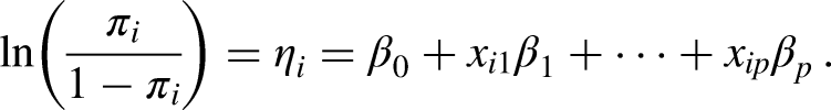
Logistic regression

For n individuals, let observations $(y_{i}, x_{i 1}, \dots, x_{i p}), i = 1, \dots, n$ of a binary target variable y and covariates $x_{1}, \dots, x_{p}$ be given. In the logistic regression model, the relationship between y and metric, categorical or binary covariates is examined. Here, $y = 1$ denotes the occurrence of a particular event (typically defined as “success”) and y = 0 that the event does not occur (also defined as “failure”). Then,

π_{i} = P (y_{i} = 1 | x_{i 1}, \dots, x_{i p}) = E [y_{i} | x_{i 1}, \dots, x_{i p}]

is the (conditional) probability for the occurrence of

y_{i} = 1

, given the covariate values

x_{i 1}, \dots, x_{i p}

. The aim is to model

π_{i}

appropriately as a function of the features.

Therefore, the linear predictor $η_{i}$ is related to the probability $π_{i}$ by a strictly monotonically increasing function $h : R \to [0, 1]$ , i.e.

π_{i} = h (η_{i}) = h (β_{0} + β_{1} x_{i 1} + \dots + β_{k} x_{i p}) .

The function

h (\cdot)

is also called the response function. With the help of the inverse function

g = h^{- 1}

, the so-called link function, we can also write

η_{i} = g (π_{i}) .

The logistic regression model is the most famous candidate within the framework of Generalized Linear Models (GLMs).

The estimators for $β_{0}, \dots, β_{p}$ are obtained by numerical maximization of the log-likelihood, e.g. by using the Fisher scoring or the Newton-Raphson method, see, e.g., Nelder and Wedderburn (1972). Generally, for more details on GLMs, see also Fahrmeir and Tutz (2001).

Regularization

If the number of covariates p becomes very large, the estimation becomes numerically unstable (see, e.g., Fahrmeir et al., 2013). This can also be the case if there is some substantial mulitcollinearity between the columns of the design matrix $X = {(x_{1}, \dots, x_{n})}^{⊤}$ . To address this problem, a penalty term pen( $β$ ) is added to the model’s (negative) log-likelihood $l (\cdot)$ , which in our case corresponds to a Bernoulli logit model. According to Park and Hastie (2007), the estimator is then obtained by minimizing

{\hat{β}}_{p e n} = \underset{β}{\arg min} (- l (β) + λ \cdot p e n (β)),

where

λ

is the penalty parameter that controls the influence of the penalty term on the parameters estimated by the ML method.

LASSO

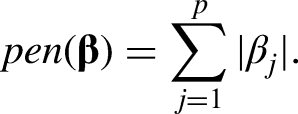
One possibility for penalization is provided by the Least Absolute Shrinkage and Selection Operator (LASSO; Tibshirani, 1996). The corresponding penalty term is given by

p e n (β) = \sum_{j = 1}^{p} | β_{j} | .

It allows model estimation and variable selection to be performed in one step, as small coefficients are shrunk to 0. No closed-form representation for solving this minimization problem does exist. Therefore, numerical optimization methods are used to obtain the optimal LASSO estimator

{\hat{β}}_{LASSO}

(see, e.g.,Friedman et al., 2010). To optimize the penalty parameter

λ

typically K-fold cross validation is used.

Spline-based approaches

In the methods introduced above, the influence of the covariates on the target variable is assumed to be strictly linear. However, often also non-linear influences are relevant. In order to model these appropriately and flexibly, so-called splines can be used. Here, the so-called B-splines (Eilers and Marx, 2021, 1996) will be employed.

B-Splines

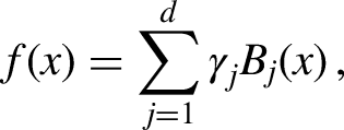
In principle, with B-splines a non-linear effect $f (x)$ of a metric predictor can be represented as

f (x) = \sum_{j = 1}^{d} γ_{j} B_{j} (x),

where

B_{j} (x)

represent the different B-spline basis functions, d denotes the number of basis functions used, and

γ_{j}

the corresponding spline coefficients. As an unpenalized estimation of a non-linear B-spline effect often overfits, typically the non-linear effect is smoothed by using penalized B-splines, i.e. P-splines.

P-splines

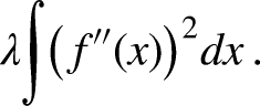
Beside the problem of potential overfitting, the goodness-of-fit of the B-spline approach depends on the number of selected nodes. To avoid this problem, various penalization methods exist in the form of P-splines. Here, a penalized estimation criterion, which is extended by a penalty term, is used instead of the usual estimation criterion. For P-splines based on B-splines (see, e.g., Eilers and Marx, 1996), the function $f (x)$ is first approximated by a polynomial spline with many nodes (typically about 20 to 40).

A suitable penalty term guaranteeing smoothness then would be given by

λ \int {(f^{″} (x))}^{2} d x .

This is motivated by the fact that the second derivative is used as a measure of the curvature of a function. If this becomes too large, it will be penalized by the term above. For approximation of the second derivative exist simple representations, so that the simpler penalty term

λ \sum_{j = 3}^{d} {(Δ^{2} γ_{j})}^{2}

could be used instead, where

Δ^{2} γ_{j} = γ_{j} - 2 γ_{j - 1} + γ_{j - 2}

(see again Eilers and Marx, 1996).

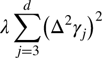
The optimal smoothing parameter $λ$ is determined using generalized CV. For more details on the methodology, see also Eilers and Marx (2021), and for more details on the corresponding software implementation in R, see Wood (2017).

Machine learning approaches

In the following, we’ll introduce different machine learning approaches that are suitable for binary responses and will be used in this work for comparison against the regression approaches, which were introduced before in Section “Regression approaches”.

Classification trees

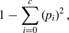
Decision trees are a supervised machine learning algorithm. A tree starts with its root node and then follows binary splits based on the features’ values until a leaf node is reached and the final binary result is given. The goal is to create a model that predicts the value of a target variable by learning simple decision rules inferred from the given features. The splitting of nodes (including the root node) to sub-nodes happens based on impurity metrics. Hence, decision trees seek to find the best split to subset the data, and they are typically trained through the Classification And Regression Tree (CART) algorithm. Metrics, such as Gini impurity and information gain can be used to evaluate the quality of the splits. CARTs were introduced by Breiman et al. (1984) and use Gini impurity in the process of splitting the data set into a decision tree. Gini impurity measures how often a randomly chosen attribute is misclassified and can be represented as follows

1 - \sum_{i = 0}^{c} (p_{i})^{2},

where

p_{i}

is the probability of class i with total number of classes c. The values of the Gini index range from 0 to 1, a lower value being more ideal. It should be noted that in this manuscript we will focus on the classification trees rather than the regression ones, as in our case the target is a binary variable (i.e. the target variable is categorical).

However, a fully grown tree typically will overfit the training data and the resulting model will not generalize well for predicting the outcome of new (unseen) test data. Therefore, techniques such as pruning (stopping the tree to grow) are used to control this problem. In the rpart package (Therneau et al., 2015), this is controlled by the complexity parameter (cp), which gives a threshold which an improvement has to pass that a split stays in the tree. A too small value of cp leads to overfitting, and a too large cp value will result in a too small tree and, hence, underfitting. Both cases decrease the predictive performance of the model. An optimal cp value can be estimated by testing different cp values and using cross-validation (CV) approaches to determine the corresponding prediction accuracy of the model¹. The best cp is then defined as the one that maximizes the CV accuracy.

Random forest

Individual trees, as Breiman (1996b) pointed out, suffer from instability, which is inherent in the tree model and can not be fixed through changing the way a tree is built. A first solution that does not interfere in the tree construction process is an ensemble method called bootstrapping and aggregating (bagging; Breiman, 1996a), which in general improves the predictive performance compared to a single regression tree and is easy to implement.

Similar to bagging, a random forest also consists of multiple decision trees which are aggregated for a more accurate prediction (Breiman, 2001). The logic behind the random forest model is that multiple uncorrelated models (i.e., the individual decision trees) perform much better as a group than they do alone, as this reduces the variance and yields more accurate predictions than an individual model. Depending on the type of problem, the type of prediction will vary. For a regression task, the individual decision trees will be averaged, and for a classification task, a majority vote, (i.e. the most frequent categorical variable) will yield the predicted class.

Again, in this manuscript, we will consider the classification task for the random forest since our target variable is binary. The main extension compared to bagging is the idea of drawing randomly only a subset of “mtry” features at each node for splitting in random forest, which involves selecting a random subset of predictors from the set of all available features at each decision node in a decision tree. This introduces diversity among the trees in the ensemble, reducing the risk of overfitting and enhances the model’s generalization performance by ensuring that each tree is built on a different subset of features. For fitting random forest models, we use the ranger implementation in R (Wright and Ziegler, 2017).

Here, in the random forest, mtry and the ntree are the two parameters that most likely to have a big effect on our final accuracy and are defined as follows:

–

mtry: number of variables randomly sampled as candidates at each split.

–

ntree: number of trees to grow.

The mtry hyperparameter controls the split-variable randomization feature of the random forests and it helps to balance low tree correlation with reasonable predictive strength. For classification $m t r y = \sqrt{p}$ is recommended, where p is the number of predictors. However, when there are fewer relevant predictors a larger value of mtry tends to perform better because it makes it more likely to select those features with the strongest signal. When there are many relevant predictors, a lower mtry might perform better. For this reason, we decided to properly tune this parameter using (self-implemented) 10-fold CV (see footnote 1 for details).

There are no specific criteria’s when it comes to choosing the number of trees that the random forest should use, as long as ntree is large enought. However, there is a threshold where adding more trees does not give any significant gain to the random forest (Oshiro et al., 2012), but computational costs would unnecessarily increase. Here, we decided to set ntree $= 400$ (and, hence, did not tune this parameter).

Extreme gradient boosting

Boosting originates in the machine learning community and proved to be a successful and practical strategy to improve classification procedures. Boosting is a sequential ensemble method that combines the predictions of multiple weak models to produce a stronger prediction, resulting in a final, aggregated model. I.e., first, a single model is built for the task and prediction errors are computed. Then, the second model is built which tries to correct the errors present in the first model. This procedure is continued and models are added until either the complete training data set is predicted correctly or the maximum number of models are added.

Since Freund et al. (1996) have presented their famous Ada-Boost algorithm, many extensions have been proposed and boosting approaches were updated to estimate predictors for statistical models (e.g., gradient boosting by Friedman et al., 2000, generalized linear and additive regression based on the L2-loss by Bühlmann and Yu, 2003).

Hence, boosting is considered as a sequential process; i.e., if e.g. (simple) trees are used as learners, those are grown using the information from a previously grown tree one after the other. This process slowly learns from data and tries to improve its prediction in subsequent iterations. A main advantage of statistical boosting algorithms is their flexibility for high-dimensional data and their ability to incorporate variable selection in fitting process (Mayr et al., 2014). An extensive and enlightening, general overview on gradient boosting algorithms can be found in Bühlmann and Hothorn (2007). Friedman (2001) introduced the idea of gradient tree boosting, using decision trees as learners. The decision trees are repeatedly fitted on the residuals of the previous fit and, hence, are combined to a sequential ensemble.

This technique was then further improved by Chen and Guestrin (2016) via introducing additional regularization in the objective function. The regularization terms make the single trees weak learners to avoid over fitting. In a certain boosting iteration, the next tree is additively incorporated into the ensemble after multiplication with a rather small learning rate which makes the learners even weaker. The method is called extreme gradient boosting, in short XGBoost, and is known in the machine learning community for its high predictive power. The approach is implemented in the xgb.train function from the xgboost R package (Chen et al., 2023). One important aspect is that XGBoost involves several tuning parameters. For this purpose, we specified reasonable, discrete grids and again used (self-implemented) 10-fold cross validation to determine optimal tuning parameters, see footnote 1 for further details.

Support vector machine (SVM)

Support vector machine (SVM) is another supervised machine learning technique, developed by Cortes and Vapnik (1995). The theory of SVM can be explained by defining four concepts, namely the hyperplane, the optimal margin, the soft margin and the kernel function (Noble, 2006): (i) the hyperplane, is the optimal line in a high dimensional space that separates the data points; (ii) the optimal margin is defined as the distance between the hyperplane and the closest support vectors; (iii) the soft margin which allows for separation of data points with a minimal number of misclassifications; (iv) as data points in a classification problem cannot always be separated linearly, the fourth concept, the kernel function, was developed. The kernel function changes the shape of space to a higher dimension and makes it possible to find a non-linear decision boundary. A kernel function that does not suggest too many unnecessary dimensions is preferred because too many dimensions can lead to over fitting. When the data is perfectly linearly separable only then we can use Linear SVM. Perfectly linearly separable means that the data points can be classified into two classes by using a single straight line. However, in case the data is not linearly separable we can use non-linear SVM. So if the data points cannot be separated into two classes by using a straight line, we use kernel functions to classify them. In most applications we do not find linearly separable data points, hence, we use kernel functions in order to solve them. In this work, two different SVM types are used for our models, namely the linear SVM and the non-linear SVM with radial basis function (RBF) kernel.

The mathematical definition of a hyperplane in two dimensions is given by James et al. (2013) as

β_{0} + β_{1} x_{1} + β_{2} x_{2} = 0,

(1)

for parameters $β_{0}$ , $β_{1}$ and $β_{2}$ . Any $x = (x_{1}, x_{2})^{T}$ for which equation (1) holds is a point on the hyperplane.

Equation (1) can be extended to the p-dimensional case by

β_{0} + β_{1} x_{1} + β_{2} x_{2} + \dots + β_{p} x_{p} = 0,

(2)

with $x = (x_{1}, x_{2}, \dots, x_{p})^{T}$ being a vector of length p. Again, if x satisfies equation (2), then x lies on the hyperplane. In case that x does not satisfy equation (2), then this indicates that x lies on one side of the hyperplane, e.g.

β_{0} + β_{1} x_{1} + β_{2} x_{2} + \dots + β_{p} x_{p} > 0.

Otherwise, if

β_{0} + β_{1} x_{1} + β_{2} x_{2} + \dots + β_{p} x_{p} < 0,

then x lies on the other side of the hyperplane.

Suppose that we have an $n \times p$ data matrix $X$ that consists of n training observations in the p-dimensional space with corresponding binary responses falling into two classes, that is, $y_{1}, \dots, y_{n} \in {- 1, 1}$ , where −1 represents one class and 1 the other class.

Then, a separating hyperplane has the property that

y_{i} \cdot (β_{0} + β_{1} X_{i 1} + β_{2} X_{i 2} + \dots + β_{p} X_{i p}) > 0

for all

i = 1, \dots, n

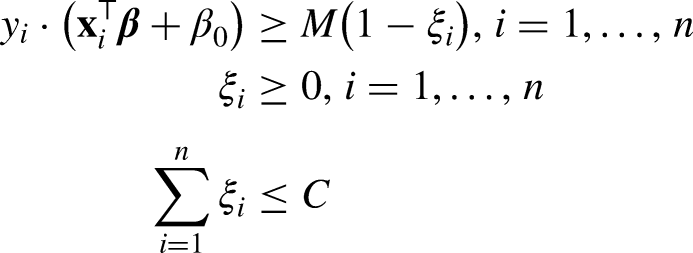
The maximal marginal hyperplane is the separating hyperplane for which the margin is largest. For a set of n training observations $x_{1}, \dots, x_{n} \in R^{p}$ and associated class labels $y_{1}, \dots, y_{n} \in {- 1, 1}$ , the maximal margin hyperplane is e.g. defined by James et al. (2013) as the solution to the following optimization problem. Let $M > 0$ represent the margin of our hyperplane. Then, we want to maximize M and optimize $β_{0}, β_{1}, \dots, β_{p}$ in

\begin{aligned} y_{i} \cdot (β_{0} + β_{1} x_{i 1} + β_{2} x_{i 2} + \dots + β_{p} x_{i p}) \geq M, \forall i = 1, \dots, n, \end{aligned}

subject to

\sum_{j = 1}^{p} β_{j}^{2} = 1

. Further details about SVM can be found e.g. in James et al. (2013).

Often classes are not perfectly separable, then so-called slack variables $ξ_{1}, \dots, ξ_{n}$ are introduced in additional constraints

\begin{aligned} y_{i} \cdot (x_{i}^{⊤} β + β_{0}) & \geq M (1 - ξ_{i}), i = 1, \dots, n \\ ξ_{i} & \geq 0, i = 1, \dots, n \\ \sum_{i = 1}^{n} ξ_{i} & \leq C \end{aligned}

with

C \geq 0

constant. Those slack variables allow some leeway compared to perfect separation, and

ξ_{i}

corresponds to the proportion of M that observation i lies on the wrong side of its margin line (see, e.g., Hastie et al., 2009). For

0 < ξ_{i} \leq 1

, observation i lies between its margin line and the hyperplane, and for

ξ_{i} > 1

it lies on the wrong side of the hyperplane. Observations on the correct side of the margin yield

ξ_{i} = 0

. Hence, C is a tuning parameter that restricts the total amount of observations that may lie on wrong sides. Only those observations with

ξ_{i} \geq 0

affect the hyperplane and are called support vectors. Note that in addition to linear SVM, there also exists a non-linear version known as the radial SVM, which will also be used in the following.

The main advantage of using SVM is that they are more effective in high dimensions where the number of features can be very large. The SVM commonly achieves better accuracy in comparison to Artificial Neural Networks (ANNs; Sipko and Knottenbelt, 2015). Furthermore, Valero (2016) explains that SVM also gives a sparse solution, which reduces the risk of overfitting. A detailed overview of the SVM approach for classification is given in Steinwart and Christmann (2008) and Wang and Casasent (2008). A manual grid search of hyperparameter values is used. Based on tuning results of the parameters for the radial basis function (RBF) kernel, the best SVM model is identified. Then the performance of the tuned SVM model is evaluated using the testing data set. This is done by using the tune.svm function from the e1071 R package (Dimitriadou et al., 2009).

Artificial neural networks (ANNs)

An artificial neural network (ANN) is a computational model inspired by the way biological neural networks in the human brain process information (Rosenblatt, 1958). ANNs were developed separately in different fields, e.g. statistics and artificial intelligence, and reach back to at least 1986 (see, e.g., McClelland et al., 1987; Rumelhart et al., 1986a, 1986b). They consist of interconnected nodes, or neurons, organized into layers: an input layer, one or more hidden layers, and an output layer. Each connection between neurons has an associated weight that adjusts as learning proceeds. In a nutshell, an ANN relies on the following components and works as follows: –

Input Layer: Data is fed into the network through the input layer.

–

Weighted Sum: Each neurone calculates a weighted sum of its inputs.

–

Activation Function: The weighted sum is passed through an activation function (e.g. ReLU or sigmoid). It can introduce non-linearity and determines the neuron’s output.

–

Forward Propagation: The output from one layer becomes the input for the next layer until reaching the output layer.

–

Loss Function: The difference between the predicted output and actual target values is calculated using a loss function.

–

Backpropagation: The network adjusts its weights based on this error using optimization algorithms like gradient descent, effectively “learning” from the data.

Through repeated iterations over training data, ANNs can learn complex patterns and make predictions or classifications on new data. A sound introduction to ANNs can be found for example in Hastie et al. (2009).

In this work, we train our ANNs using the R function neuralnet (Fritsch et al., 2019). The function allows to use backpropagation, resilient backpropagation (with or without weight backtracking) or a modified globally convergent version. Moreover, it enables flexible settings through custom-choice of error and activation function.

Further modelling details and evaluation aspects

In the following, some more details on the regression model approaches, which seem to be suitable to adequately model tennis matches, are provided. Then, both the regression and machine learning approaches are investigated and compared with respect to their predictive performance on new, unseen matches. To achieve this, a leave-one-tournament-out CV-type approach is employed to select the best model based on various performance measures. In an external validation using previously unused data, the top models from the earlier CV-type strategy are assessed through an expanding window method. Subsequently, a rolling window with a recent three-year training dataset is utilized to make predictions for the selected models. For all computations and evaluations the statistical programming software R (R Core Team, 2023) was used.

Modeling details for the regression approaches

In this section, we provide more details for the regression approaches. These can also be found in Buhamra et al. (2024), but for better readability of this manuscript we describe them here again.

Principally, to model the binary outcome y (win/loss) of a tennis match, the logistic regression models introduced in Section “Regression approaches” can be employed, which generally are given by

\ln (\frac{π_{i}}{1 - π_{i}}) = η_{i} = β_{0} + x_{i 1} β_{1} + \dots + x_{i p} β_{p} .

Since the

x_{i 1}, \dots, x_{i p}, i = 1, \dots, n,

are differences of the covariates of both players, i.e. the value of the second player always being subtracted from the one of the first player,

β_{0}

would represent a “home effect” of the first-named player. However, since the ordering of the two players in our dataset is random,

β_{0}

is not meaningful and, hence, excluded (i.e.,

β_{0}

is set to zero). Finally, the

y_{i} | x_{i 1}, \dots, x_{i p}

are assumed to be independent for

i = 1, \dots, n

Linear effects

The simplest model approach assumes linear covariate effects in the predictor, but requires careful selection of covariates. For this purpose, all possible combinations of the available variables are compared in the CV-type strategy. With seven covariates in the dataset, there are initially $\sum_{i = 1}^{7} (\begin{matrix} 7 \\ i \end{matrix}) = 127$ combinations; however, since three of these reflect specific age differences, we ensure that maximum one age variable can be incorporated in each combination. This leads to a total of 63 distinct combinations.

Non-linear effects (splines)

As the assumption of strictly linear effects can possibly be very restrictive, spline models using B-splines are also considered. These enable to incorporate non-linear covariate effects. Again, we regard the same 63 covariate combinations, and again compare the respective models in terms of various performance measures. To obtain smoothness, the splines are penalized via using P-splines. Moreover, an additional regularization approach is used, i.e. additional variable selection is performed on the spline effects by potentially setting the corresponding spline coefficients to zero. This is implemented in the gam-function from mgcv (Wood, 2017) (via setting the select argument to TRUE). The underlying methodology of this additional penalization and variable selection approach is described e.g. Marra and Wood (2011).

Surface-specific player skills

Tennis matches are played on different surfaces (grass, hard court, and clay), each influencing match outcomes differently. Hence, it is reasonable to assume that players’ performances vary across these surfaces. For instance, Rafael Nadal, known as the “king of clay”, has won 14 French Open titles but only two Wimbledon titles on grass. Conversely, Roger Federer has won Wimbledon eight times but just once at the French Open. As already described in Buhamra et al. (2024), we account for these player-surface dynamics by creating a corresponding factor variable using effect encoding. This involves adding artificial columns to the dataset with entries

\in {- 1, 0, 1}

for each player-surface combination; a player can have up to three such columns. If a player has not competed on a surface, the respective column is omitted. Each row contains one entry of 1 and of -1, while all other entries are 0. The entry 1 indicates the first player’s combination with the match surface, while -1 corresponds to the second player’s combination. For example, the line in the subsequent table

$\dots$	$N a d a l . H a r d$	$N a d a l . G r a s s$	$N a d a l . C l a y$	$\dots$	$F e d e r e r . H a r d$	$F e d e r e r . G r a s s$	$F e d e r e r . C l a y$	$\dots$
$\dots$	0	1	0	$\dots$	0	−1	0	$\dots$

represents a match where Rafael Nadal played against Roger Federer on grass, with Nadal being first-named and Federer second-named. All other entries in that row are 0, as the match was played on grass and only these two players were involved. All these columns are added to our data set, and are used as new features in combination with the existing variables age, ranking, points, Elo, prob, age.30 and age.int.

This results in a large number of new covariates, namely 1,024, and hence leads to an extremely large number of parameters being estimated, and the associated estimators become unstable. Hence, we combine the logistic regression model with LASSO regularization (see Section “Regression approaches”). Consequently, this modling approach is restricted to linear covariate effects. These surface-specific player abilities allow the model to detect players who have won or lost more often than average on a specific surface.

Global player skills (LASSO)

Analogously, and again following Buhamra et al. (2024), one could simply allow for global player-specific abilities, to account for players who overall perform even better or worse than the information of their covariate values would suggest (independent from a specific surface type). Similar to the previous paragraph, this can be done by introducing a corresponding factor variable, again via effect coding. Now, only one column per player is added. These columns again only have entries

\in {- 1, 0, 1}

, with 1 and −1 occurring exactly once per row. Again, in each row, the values 1 and −1 appear at the positions corresponding to the first-named and the second-named player, respectively, and all remaining entries are 0. The following exemplary row

$\dots$	$N o v a k . D j o k o v i c$	$\dots$	$R a f a e l . N a d a l$	$\dots$	$R o g e r . F e d e r e r$	$\dots$
$\dots$	0	$\dots$	−1	$\dots$	1	$\dots$

indicates that Rafael Nadal played as second-named player against the first-named player Roger Federer. For example, the entry in Novak Djokovic’s column is then 0 (as well as for all other players), since he was not involved in that particular match. Again, those global player-specific abilities are then added to the design matrix and used along with the basic covariates defined in Section “Data”. Consequently, again a large number of new covariates is obtained, namely 426, and, hence, a large number of player-specific skill parameters has to be estimated. Once more, we extend the logistic regression model with LASSO penalization and assume linear covariate effects only.

Modeling details for the machine learning approaches

For all the ML models introduced in Section “Machine learning approaches”, no player-specific dummies have been included. Also note that all tree-based approaches implicitly incorporate both non-linear as well as interaction effects. While linear SVM only accounts for linear effects, radial SVM also allows for a certain extend of non-linearity.

Benchmark model

Similar to Buhamra et al. (2024), we built a benchmark model for prediction based on the probabilities (probs) calculated from the average odds of the different bookmakers included in the 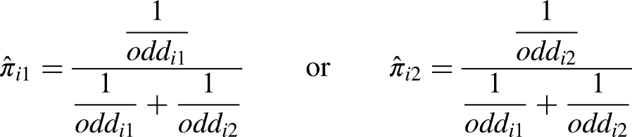deuce package. According to e.g. Schauberger and Groll (2018), estimates for the winning probabilities of both players, ${\hat{π}}_{i 1}$ and ${\hat{π}}_{i 2}$ , for match i can be derived from the two corresponding winning odds, $o d d_{i 1}$ and $o d d_{i 2}$ , as follows:

{\hat{π}}_{i 1} = \frac{\frac{1}{o d d_{i 1}}}{\frac{1}{o d d_{i 1}} + \frac{1}{o d d_{i 2}}} or {\hat{π}}_{i 2} = \frac{\frac{1}{o d d_{i 2}}}{\frac{1}{o d d_{i 1}} + \frac{1}{o d d_{i 2}}}

Naturally, we have

{\hat{π}}_{i 1} + {\hat{π}}_{i 2} = 1

, adjusting for the bookmaker’s margins, which result from the fact that the betting providers artificially lower their betting odds to gain some profit. This means that when the inverse values of the original odds are directly used as probabilities, they do not sum up to 1, but to a value slightly larger than 1. Hence, the sum of the reciprocals in the denominator is used for normalization, assuming implicitly that the margin is equally distributed to both players.

Performance measures

To compare the predictive performance of the used regression and machine learning models on new, unseen data, several measures are considered (see also Buhamra et al., 2024). First, let ${\tilde{y}}_{1}, \dots, {\tilde{y}}_{n}$ denote the true binary outcomes of the n matches, i.e., ${\tilde{y}}_{i} \in {0, 1}, i = 1, \dots, n$ . Second, let ${\hat{π}}_{i 1} = : {\hat{π}}_{i}$ denote the probability, predicted by a certain model, that Player 1 wins the i-th match. Since ${\tilde{y}}_{i}$ is binary, the probability that Player 2 wins the match then simply yields ${\hat{π}}_{i 2} = 1 - {\hat{π}}_{i 1}$ .

Classification rate

The (mean) classification rate gives the proportion of matches correctly predicted by a certain model, i.e.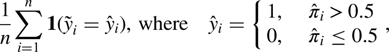

\frac{1}{n} \sum_{i = 1}^{n} 1 ({\tilde{y}}_{i} = {\hat{y}}_{i}), where {\hat{y}}_{i} = {\begin{matrix} 1, & {\hat{π}}_{i} > 0.5 \\ 0, & {\hat{π}}_{i} \leq 0.5 \end{matrix},

see, e.g., Schauberger and Groll (2018). Hence, large values indicate a good predictive performance.

Predictive Bernoulli likelihood

The (mean) predictive Bernoulli likelihood is based on the predicted probability 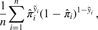${\hat{π}}_{i}$ for the true outcome ${\tilde{y}}_{i}$ , and for n observations is defined as

\frac{1}{n} \sum_{i = 1}^{n} {\hat{π}}_{i}^{{\tilde{y}}_{i}} (1 - {\hat{π}}_{i})^{1 - {\tilde{y}}_{i}},

see again Schauberger and Groll (2018). Once again, a large value is an indicator of a good model.

Brier score

The Brier score is based on the squared distances between the predicted probability 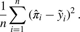${\hat{π}}_{i}$ and the actual (binary) output ${\tilde{y}}_{i}$ from match i, and according to Brier (1950) is defined as

\frac{1}{n} \sum_{i = 1}^{n} ({\hat{π}}_{i} - {\tilde{y}}_{i})^{2} .

As this is an error measure, here low values indicate a good model.

Interpretable machine learning

Next, we briefly introduce two methods from the field of interpretable machine learning (IML), namely partial dependence plots (PDP; see Friedman, 2001) and individual conditional expectation (ICE) plots (Goldstein et al., 2015). These allow to make complex, black box-type machine learning models more interpretable by understanding the marginal effects of individual features (see R packages pdp by Greenwell et al., 2017). More details on IML are provided in Molnar (2020).

Partial Dependence Plot (PDP)

Following Friedman (2001), PDPs display the marginal effect of one or two predictors on the predicted response of a ML model, which might be linear, monotonic, or strongly non-linear. In the notion of Molnar (2020), the partial dependence function is given by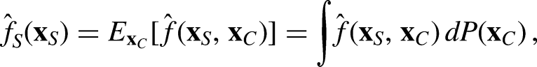

{\hat{f}}_{S} (x_{S}) = E_{x_{C}} [\hat{f} (x_{S}, x_{C})] = \int \hat{f} (x_{S}, x_{C}) d P (x_{C}),

where

P (\cdot)

is the density of the features in set C,

x_{S}

are the predictors from the (typically small) set S for which

{\hat{f}}_{S} (\cdot)

is desired, while

x_{C}

denotes the remaining predictors included in the underlying ML model

\hat{f} (\cdot)

. By integrating out the influence of the features from C, we obtain the marginal effects of the features of interest in S, still taking into account potential interactions.

For given training data of size n and an arbitrary value of the features from S, ${\hat{f}}_{S} (\cdot)$ can be estimated via

{\hat{f}}_{S} (x_{S}) = \frac{1}{n} \sum_{i = 1}^{n} \hat{f} (x_{S}, x_{i, C}),

i.e. by their marginal effect on the response, averaging over the observed values

x_{i, C}

of the remaining predictors. An important underlying assumptions is that the covariates from the two different set C and S are uncorrelated in order to avoid unrealistic estimates.

Individual Conditional Expectation (ICE)

Closely related to PDPs, ICE plots illustrate the effect of a certain predictor on the individual observation level (Goldstein et al., 2015). The plot contains one line per observation, representing the predicted response for this observation as the covariate of interest varies. Hence, the ICE plot reveals the variability and heterogeneity of the covariate effects across different all individual obersvations. This way, interpretability and transparency of a complex ML model can be increased and outliers identified. Moreover, possible interactions between different covariates may be detected.

Results

In the following, the proposed regression models along with the machine learning techniques are compared using the various performance measures introduced in Section “Performance measures”. This is done separately via a leave-one-tournament-out cross validation strategy (Section “Leave-one-tournament-out cross validation”), as well as both via an expanding window (Section “Expanding window validation”) and a rolling window external validation scenario (Section “Rolling window validation”).

Leave-one-tournament-out cross validation

In a first step, to evaluate the models only the Grand Slam tournaments from 2011 to 2021 are used, i.e. the tournaments that took place in 2022 are initially not considered and are used as external validation data later on (see Section “Expanding window validation”). So, from each of the eleven years four tournaments are used with the exception of year 2020, where Wimbledon did not take place due to the COVID-19 pandemic. This results in a sub data set, which contains 4,720 observations, on which a 43-fold CV-type strategy is performed based on the following scheme (similar to Buhamra et al., 2024):

From the 43 Grand Slam tournaments present in the data set, a training data set of 42 tournaments and a test data set of the remaining tournament are constructed.

Then, all regression and machine learning models introduced above are fitted: –

For the models with linear influences, the function glm from the R package stats (R Core Team, 2022) is used. As described in Section “Modeling details for the regression approaches”, there are 63 such models, each using at most one of the three variables for age.

–

For the calculation of the spline models the function gam from the R package mgcv (Wood, 2004) is used. Again, there are also 63 different models here.

–

In order to be able to compute the two LASSO-penalized models, first the design matrices have to be constructed as described in Section “Modeling details for the regression approaches”. For a proper usage of the LASSO, then all columns of the design matrix of the training data need to be standardized (including also those columns corresponding to the surface-specific and global player skills).The function cv.glmnet from the R package glmnet (Friedman et al., 2010) is used to compute both models. For this, a 10-fold (inner) CV is first performed on the current training data to find the optimal $λ$ which provides the minimum deviance. The corresponding LASSO model is used afterwards for prediction. 10-fold CV is also recommended in Friedman et al. (2010).

–

The random forest model is fitted via the R package ranger (Wright et al., 2019), the classification trees are trained using rpart pakage (Therneau et al., 2015), wheres for the XGBoost model the respective xgboost implementation is used (Chen et al., 2019), For SVM the e1071 package is employed, see (Meyer et al., 2024). Note that for the aforementioned ML models, no player-specific dummies have been included, as the results did not improve (result not shown). Finally, for ANNs the neuralnet package is used (Fritsch et al., 2019). Actually, they even partly deteriorated. Also note that the tree-based approaches implicitly incorporate both non-linear and interaction effects.

After fitting the respective model, for each match of the test data the probabilities that the first player wins are predicted.

Steps 1–3 are repeated until each of the 43 tournaments has once been used as test data set.

Finally, the predicted results are compared with the actual results and the performance measures defined in Section “Performance measures” are calculated.

Table 1 shows the results of the five best models with linear effects and the five best models with spline effects². Additionally, the results of the LASSO models, all machine learning approaches and the benchmark model are shown. The models are listed below in such a way that the best model is determined in first place, the second best in second place and so forth.

Table 1.

Results of the leave-one-tournament-out CV approach for the five best models per regression model class, as well as for the machine learning, LASSO approaches and the benchmark model; best performer in bold font.

	Modelling approach	Class.	Likeli-	Brier
	Modelling approach	rate	hood	score
Linear	Prob	0.7772	0.6919	0.1549
	Rank, Prob	0.7776	0.6918	0.1550
	Points, Prob	0.7772	0.6917	0.1549
	Rank, Points, Prob	0.7772	0.6917	0.1550
	Age, Prob	0.7766	0.6918	0.1550
Splines	Prob	0.7764	0.6912	$0.1546$
	Rank, Prob	0.7764	0.6912	$0.1546$
	Points, Prob	0.7764	0.6912	0.1547
	Rank, Points, Prob	0.7764	0.6912	0.1547
	Elo, Prob	0.7764	0.6911	0.1547
Machine learning	ANN	$0.8021$	0.6828	0.1560
	Random forest	$0.7978$	0.6817	0.1584
	SVM (Linear)	0.7961	$0.7415$	0.1675
	SVM (Radial kernel)	0.7829	0.6149	0.1807
	XGBoost	0.7777	0.7234	0.1901
	Classification tree	0.7486	0.6703	0.2178
LASSO	Surface specific	0.7774	0.6816	0.1551
	General skills	0.7770	0.6838	0.1551
	Benchmark	0.7772	0.6709	0.1555

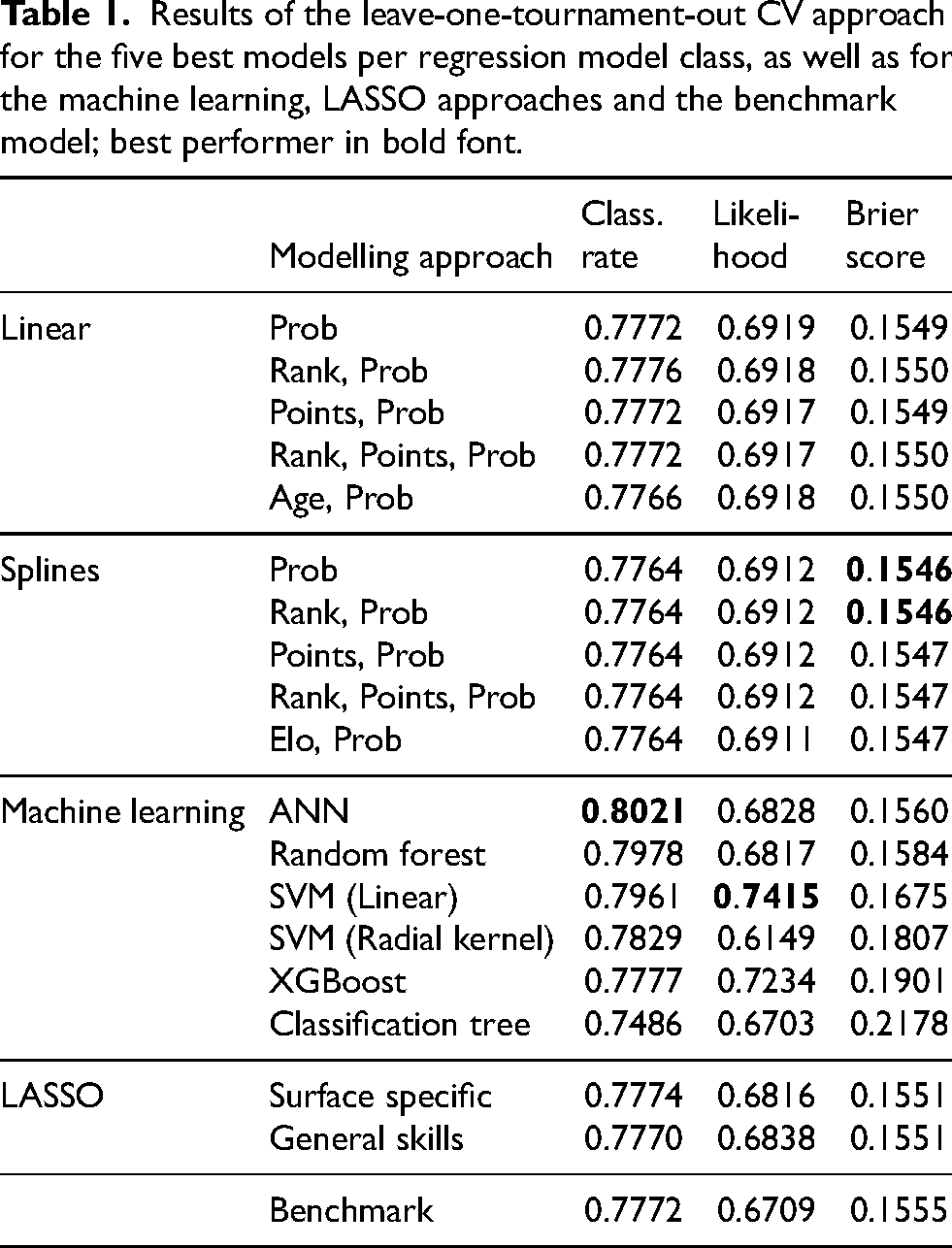
The classification rate is above 77% for all models, except for the classification tree (see 1st column). It is noticeable that within each group of model approaches the classification rate is almost the same (differences are only seen in the fourth decimal). However, for the machine learning models the values vary more. The neural network performs best with a value of 0.8021, i.e. this model predicts the correct outcome for 80.21% of the matches. In second place is the RF model, which has a correct prediction value of 0.7978. Also, it is noticeable that all spline models perform (almost) equal with a value of 0.7764. In addition, with respect to the classification rate, four different models deliver the same value of 0.7772.

For the (average) predictive Bernoulli likelihood (2nd column) we obtain a somewhat similar picture. The mean likelihood of the models with both linear and non-linear effects is slightly larger than 0.69, i.e. the models predict the correct outcome with an average probability of about 69%. The two LASSO models are just below 0.69. It is noticeable that the linear SVM model achieves the largest predictive likelihood, which is 0.7415. Again, the spline models performed almost identical with a value of about 0.691.

Across model groups, similar to the classification rate the differences in the Brier scores are rather small. The models with non-linear effects perform best in this regard, with Brier scores between 0.1546 and 0.1547. The models with linear effects produce slightly larger values, followed by the LASSO models and then the machine learning models. Here, the two LASSO models delivered the same value of 0.1551. The classification tree performs clearly worst with a value of 0.2178, followed by XGBoost and the SVM (with radial kernel) with values of 0.1901 and 0.1807, respectively.

Overall, the results show that the spline models with only prob or both rank and prob as covariates, the ANN and the linear SVM perform best across all performance measures.

Expanding window validation

Next, we will validate the models from above with respect to their predictive performance on new, unseen test data in a more realistic way. For this purpose, we investigate the three best models from the groups of modelling approaches with linear and non-linear effects, as well as the two LASSO models, the machine learning models and the benchmark model. Again, all performance measures are calculated on the four Grand Slam tournaments 2022, which contains overall 293 matches. To mimic a more realistic prediction use case, this time the validation is performed using an expanding window forecasting approach, i.e. each time one of the remaining tournaments is used as the test data set in chronological order, and the training data set is constantly updated and enlarged. Altogether, this scheme has already been used in Buhamra et al. (2024) and can be explained as follows:

First, all tournaments prior to 2022 are used as the training data set. Then, all models are fitted as described in step 2 of the CV approach described in Section “Leave-one-tournament-out cross validation”. Based on those, predictions are derived for the 2022 Australian Open matches, as this was the 1 $^{st}$ Grand Slam tournament in 2022.

Then, the training data is updated, by adding the matches of the Australian Open 2022 on which the models are fitted again and predictions are made for the French Open 2022, which is the 2^nd Grand Slam tournament in 2022.

Next, the matches of the French Open 2022 are added to the training data set and the models are fitted again. Based on those fits, Wimbledon 2022 is predicted.

Then, the Wimbledon 2022 matches will be added to the training data set, and again, the models are fitted and predictions are made for the final Grand Slam tournament in 2022, the US Open 2022.

Finally, the prediction results for all four tournaments are compared with the actual match outcomes, and the corresponding performance measures are calculated (see Table 2 for results).

Table 2.

Results of the expanding window approach for the best three regression models out of those five best models found Section “Leave-one-tournament-out cross validation”, as well as machine learning, LASSO approaches and the benchmark model; best performer in bold font.

	Modelling approach	Class.	Likeli-	Brier
	Modelling approach	rate	hood	score
Linear	Rank, Prob	0.7816	0.7037	0.1418
	Prob	0.7816	0.7036	0.1419
	Points, Prob	0.7747	0.7027	0.1421
Splines	Points, Prob	0.7782	0.7033	$0.1411$
	Prob	0.7782	0.7031	0.1413
	Rank, Prob	0.7782	0.7031	0.1413
Machine learning	SVM (Linear)	0.8295	$0.7637$	0.1446
	XGBoost	$0.8306$	0.7526	0.1562
	Random forest	0.8162	0.6734	0.1511
	SVM (Radial kernel)	0.7956	0.5858	0.1882
	ANN	0.7918	0.6904	0.1466
	Classification tree	0.7577	0.6803	0.2061
LASSO	General skills	0.7782	0.6969	0.1416
	Surface specific	0.7782	0.6934	0.1423
	Benchmark	0.7816	0.6810	0.1441

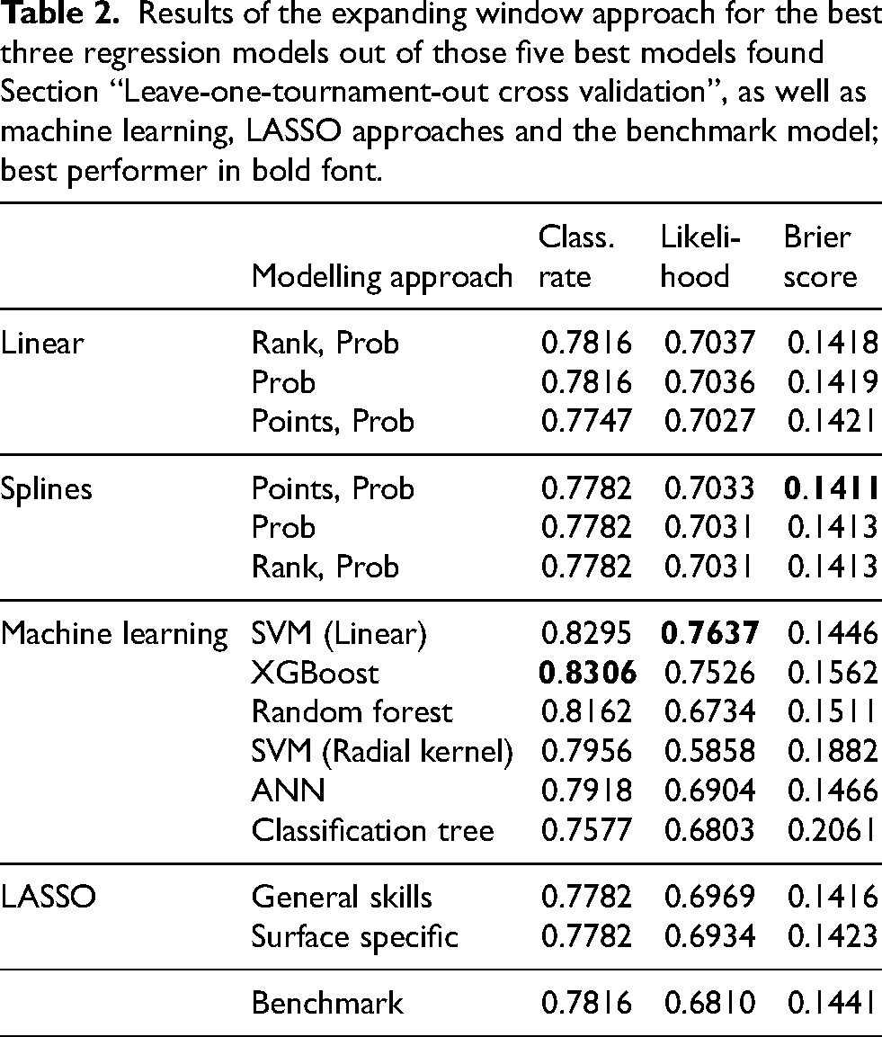
Regarding the classification rate, most of the models performed better here compared to the classification rates from the CV-type strategy from above. However, here the classification tree model delivers the worst results with a value of 0.7577, while the best value is 83.06% and is achieved by the XGBoost model. Now, the benchmark model is not among the best.

Similar trends as in Table 1 (cf. page 17) can be seen for the predictive likelihood, although the results here have generally slightly improved. XGBoost together with linear SVM achieve the largest likelihood, where the linear SVM model delivers the best value with 0.7637, only slightly behind are the linear and spline regression models that perform almost equally (all around between 0.7031 and roughly 0.7037): in case of the linear models the differences appeared in the third decimal, while in case of non-linear effects the differences can be seen only in the fourth decimal. Also, it should be noted that two of the spline models deliver the same value of 0.7031. Both the benchmark model and the LASSO models yield an even slightly smaller likelihood. The LASSO models perform almost equally with differences that can be seen only in the third decimal place. The SVM model with radial kernel here performs worst.

For most of the models the Brier score is $\in [0.1411 - 0.1441]$ , except for the machine learning models, where the values differ more. Compared to Section “Leave-one-tournament-out cross validation”, the values are slightly smaller. The classification tree model again yields the largest, and thus worst value with 0.2061. The best value is 0.1411 and is achieved by the non-linear model including covariates points and prob.

Overall, interestingly almost all approaches have improved, some even quite substantially. This indicates that the predictions should occur in chronological order. This time the results show that the spline models with both points and prob as covariates, XGBoost and linear SVM perform best, each with respect to one of the performance measures. Overall, also the linear model with only prob performs quite well. Altogether, the expanding window strategy seems to be clearly superior compared to the CV-type strategy.

Rolling window validation

An alternative strategy is to only use recent data for prediction, but in a rolling window manner. Hence, only 3 years of training data are used, i.e. 12 tournaments in total, starting from the first tournament in 2011, which is Australian open, until we reach the last tournament of 2013, which is US open. This means we use the 12 tournaments from 2011 to 2013 as first training data set and then predict the 13th tournament (i.e., the first tournament of 2014, which is Australian Open). Then, a rolling window approach is performed and the training data set constantly changes with a fixed short time window of three years. We again focus on the three best models from the groups of linear and non-linear regresion models, as well as the two LASSO models, the machine learning models and the benchmark model. In detail, this scheme can be explained as follows:

The tournaments of the first 3 years in our data set, 2011 - 2013, are used as training data, on which the models are fitted. Then, predictions can be obtained for the 2014 Australian Open, the 13^th tournament in our data set and first Grand Slam tournament in 2014.

The new training data set then shifts by one tournament and starts from the 2^nd tournament for 2011, which is French Open 2011 and ends with the 13^th tournament, i.e. Australian Open 2014. Again, all models are fitted and used to predict the next tournament, which is now the 14^th tournament in our data set (and 2^nd Grand Slam tournament in 2014).

This procedure is repeated until finally, the last training data consists tournaments 35-46 from our full data set, on which again all models are fitted and used to predict the very last tournament in our data, which is the 47^th tournament, namely the final Grand Slam tournament in 2022, US Open 2022.

Finally, the predicted results for all tournaments, on which predictions have been made, starting from Australian open 2014 until the US open 2022, are compared with the actual results and the respective performance measures are calculated. The results of the rolling window are shown in Table 3.

Table 3.

Results of the rolling window approach for the best three regression models out of those five best models found Section “Leave-one-tournament-out cross validation”, as well as machine learning, LASSO approaches and the benchmark model; best performer in bold font.

		Class.	Likeli-	Brier
	Modelling approach	rate	hood	score
Linear	Prob	0.7743	0.6893	0.1562
	Points, Prob	0.7740	0.6890	$0.1546$
	Rank, Prob	0.7714	0.6884	0.1563
Splines	Rank, Prob	0.7727	0.6895	0.1564
	Points, Prob	0.7719	0.6887	0.1566
	Prob	0.7708	0.6884	0.1563
Machine learning	SVM (Linear)	$0.8012$	$0.7424$	0.1709
	Random forest	0.7971	0.6727	0.1608
	XGBoost	0.7755	0.7231	0.2074
	SVM (Radial kernel)	0.7729	0.5448	0.2139
	ANN	0.7726	0.6837	0.1554
	Classification tree	0.7256	0.6900	0.2678
LASSO	Surface specific	0.7735	0.6735	0.1564
	General skills	0.7727	0.6753	0.1565
	Benchmark	0.7743	0.6683	0.1567

Principally, the results are quite similar compared to the previous results, but have all deteriorated a bit. The classification rate is again slightly above 77% for all models, with differences mostly only in the third decimals, except for the machine learning models which partly perform better (random forest and linear SVM). Here, linear SVM performs best with a value of 0.8012, i.e. this model predicts the correct outcome for 80.12% of the matches. Also, the random forest model here delivered good performance with a value of 0.7971. All non-linear models performed very similar, with differences that can bee found only in the third decimal place. The two LASSO models also achieved very similar values around 0.773. While three other models deliver a value around 0.774.

Compared to the results in Table 2, the predictive likelihood results are somewhat lower here. The best value is achieved by the linear SVM model (0.7424), followed by XGBoost with a value of 0.7231. The differences in both linear and non-linear regression model can only be seen in the third decimal. Both LASSO models yield very similar results around 0.67. The SVM with radial kernel and the benchmark model perform worst with values of 0.5448 and 0.6683, respectively.

Also the Brier score values are slightly worse (i.e., larger) compared to the previous results from Table 2. This clearly indicates that for a good predictive performance on Grand Slam matches, training data should be rather large, and a collection of three years of Grand Slam matches data as used here is not sufficient. Hence, besides the precise choice of statistical or machine learning approach, a sound basis of informative covariates and large enough sample sizes are very important. The classification tree model once again yields the worst value with 0.2678. The linear model including covariates points and prob is achieved the best value of 0.1546. However, all linear and non-linear regression models, the tow LASSO models and the benchmark model deliver roughly similar values with differences that can be seen only in the fourth decimal. All machine learning models instead result in rather large values, but linear SVM, random forest and neural network still yield acceptable results.

Interpretable machine learning

In the following, interpretable machine learning (IML) is used to analyze the performance of XGBoost model, which achieved the largest classification rate among all models, with a value of 0.8306, as discussed in Section “Expanding window validation”. For this purpose, combined partial dependence plots (PDPs; Friedman, 2001) and Individual Conditional Expectation (ICE; Goldstein et al., 2015 plots are presented to enhance the interpretability and visualization of the respective complex model. For the implementation in R, we rely on the pdp package (Greenwell et al., 2017). Also, we use the ggplot2 (Hadley, 2016) to create custom PDPs and ICE plots. In Figure 1, a multi-panel plot is presented where each panel represents the combined PDP and ICE plot for a different covariate (namely, age.30, Elo, points and rank). The x-axis of each panel represents the respective covariate (recall that we account for differences), while the y-axis shows the corresponding predicted winning probabilities. This visualization helps in understanding how each predictor variable individually influences the predicted outcome, highlighting potential non-linear relationships captured by the model. The ICE plot (gray lines) shows how predictions vary for individual instances, while the PDP (bold black line) displays the overall average effect of the variable.

Figure 1.

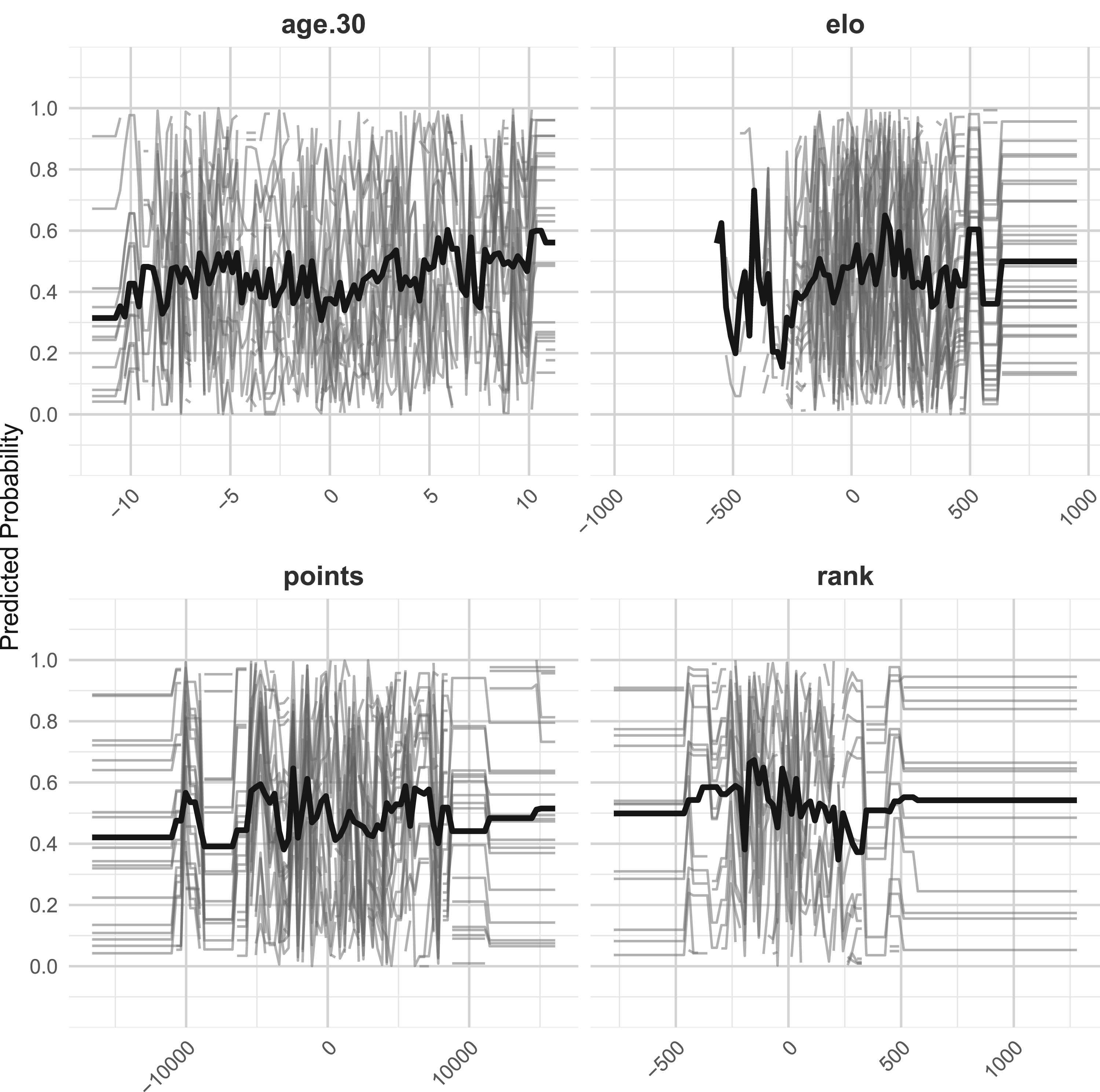
Combined PDP (thick black line) and ICE plots (gray lines) for XGBoost model in combination with the expanding window approach, including covariates age.30, Elo, points and rank.

The steep increasing trend for the Elo panel in the PDP line indicates that as Elo differences increase, the predicted probability of Player 1 winning also increases. Regarding the ICE lines, as they vary widely, the impact of Elo difference is not consistent across all matches, possibly due to interactions with other features. For the rank, PDP line decreases with increasing rank difference, which means that when Player 1 has a worse ranking, his predicted probability of winning decreases. The PDP for age.30 shows a slightly increasing trend at the beginning, then a slight decrease, indicating that age difference does not have a substantial impact on predictions. Toward the end, we observe another obvious fluctuating trend. This could mean that the impact of extreme age differences is inconsistent.

For covariate points, the PDP line also fluctuates rather strongly, indicating that the effect of the points difference on the predicted probability of winning is not straightforward, i.e., there could be ranges where having a larger points advantage helps, but other ranges where the effect is weaker or even reversed. Another explanation could be that the impact of the points difference correlates with other covariates like surface, age, or Elo rating. For example, a player with a small points advantage might have a higher winning probability on clay courts, but not necessarily on grass courts (i.e., there is an interaction effect with other features).

Summary and overview

In this manuscript, we continued the work from Buhamra et al. (2024) and modelled tennis matches in Grand Slam tournaments within the framework of regression and modern machine learning approaches. For this purpose, the same data set as used in Buhamra et al. (2024) was analyzed, which was build based on the deuce R package (Kovalchik, 2019). The final data set contains information on 5,013 matches in 47 men’s Grand Slam tournaments from the years 2011-2022, and includes covariate information on the age difference of both players, the difference in their rank positions and ATP points, in Elo rating, in probabilities for the victory of the players, calculated from the average odds by the betting providers (prob), as well as the two additional age variables, age.30 and age.int, which take into account that the optimal age of a tennis player is between 28 and 32 years.

Different regression models, which were already considered in Buhamra et al. (2024), were compared to modern machine learning approaches for modelling and prediction of tennis matches. As the outcome in tennis is binary (win or loss), the probability of the first-named player to win is modelled. It was discussed that for the logistic regression approaches, modelling with intercept is not suitable, as this would incorporate a kind of home effect for the first-named player - a property which was not desired here.

The different modelling approaches were compared in (i) a 43-fold leave-one-tournament-out CV-type strategy, (ii) an expanding window, and (iii) a rolling window validation strategy (with a short window for a period of three years). The following regression and ML approaches were included: –

Logistic regression with linear effects: all possible combinations of the seven covariates, such that at most one of the three age variables was incorporated, were considered. This resulted in 63 models.

–

Logistic regression with non-linear effects (splines): Again, the same 63 models were considered.

–

A model taking into account surface- and player-specific effects. Due to the large amount of unknown parameters, here LASSO penalization was used.

–

A model taking into account general player-specific abilities. Again, LASSO penalization was used.

–

Different machine learning approaches: classification trees, random forest, XGBoost, support vector machine with linear and radial kernel, and ANNs.

–

A benchmark model, where the predicted probabilities were derived from average betting odds.

Within the CV-type approach, the models were compared in terms of the classification rate, the predictive Bernoulli likelihood, and the Brier score. Since 63 different models resulted for each of the first two approaches, the five best models were selected in each case.

It was found that the selected linear and spline models performed very similarly in terms of classification rate, likelihood and Brier score. The classification rate was slightly above $77 %$ for all models, meaning that the models predicted the correct outcome in about $77 %$ of the matches. The predictive Bernoulli likelihood was about 0.69, while the LASSO models and the benchmark model were slightly below. The models thus predicted with an average probability of about 69% the correct outcome of a match. The Brier score was above 0.154 for all models, and differences were mostly found either in the third or fourth decimal. Regarding the machine learning models the values for the Brier score were more volatile.

The tournaments in 2022 were then used as an external validation data set in an expanding window validation approach. The three best models with each linear and non-linear effects, the two LASSO models, all machine learning models and the benchmark model were then compared again. Principally, the results of the preceding CV-type competition could be mostly confirmed, but surprisingly the expanding window strategy turned out to be clearly superior compared to the CV-type strategy: the classification rate was around $0.757 - 0.831$ , the predictive likelihood yielded around $0.681 - 0.764$ , and the Brier score was between $0.141 - 0.206$ . Obviously, performances of the models vary across measures. The XGBoost has the best performance among all others when considering the classification rate. The (linear) SVM model achieves the best predictive performance in terms of the predictive likelihood. Meanwhile, the spline model, including both covariates points and prob, outperformed all other models by yielding the lowest Brier score value.

In order to use more recent data sets for prediction, we also investigated a rolling window approach, which was based on a training data containing 12 tournaments and which was used to always predict the next tournament. The same selection of models as for the expanding window validation approach was analyzed. Principally, the results of the preceding expanding window-strategy competition could be mostly confirmed, with the values of the performance measures generally being slightly worse. The classification rate was around between $0.771 - 0.801$ , the predictive likelihood yielded around $0.545 - 0.742$ , and the Brier score was between $0.154 - 0.268$ . Again, the values somewhat differ between models and proposed performance measures. If we consider the classification rate and the predictive likelihood, then the (linear) SVM model outperforms all other models. However, for the Brier score, the linear regression model including points and prob achieves the best performance.

So, interestingly, our analyses show that for the prediction of Grand Slam tennis matches, while there are slight differences across different statistical and machine learning approaches, the specific forecast strategy used seems to play an even more important role. It turned out that on our data, an expanding window approach was clearly superior compared to two other forecast strategies. The results show that on the one hand, it seems to be important to do the predictions in chronological order, as the expanding window approach clearly outperforms the CV-type strategy. On the other hand, the training data needs to be rather large, and three years of training data as used in our rolling window approach are not sufficient. Particularly, complex machine learning methods such as SVM and XGBoost, which involve an extensive tuning process, seem to benefit from these two aspects to fully exploit their potential, as they exhibit rather good predictive performance (see Table 2). These findings are consistent with the generally known result that feature engineering tends to be the more critical choice for the modeller than the choice among strongly related models.

In the same direction heads a certain feature engineering-type approach, namely Statistical enhanced learning (SEL), which is based on so-called “statistical enhanced covariates”, could be investigated. These covariates are not directly observed, but obtained by performing certain steps of feature engineering, or even as statistical estimators from separate statistical model, see Felice et al. (2023) for more details. For example, in the context of modelling soccer, Ley et al. (2019) proposed a model to estimate flexible, time-varying team-specific ability parameters. The resulting estimates were then added to the set of (conventional) features in a random forest model, which turned out to be quite sucessful for predicting the FIFA World Cup 2018 in Groll et al. (2019). A first attempt to carry over this idea to tennis is sketched in Buhamra and Groll (2025). Moreover, we are currently working on extending the approach from Ley et al. (2019) to professional tennis (see Bartmann et al., 2025). In future research, we plan to investigate the predictive potential of such “statistical enhanced covariates” in more detail and to combine the methods proposed here with the player-specific ability parameters obtained with the approach from Bartmann et al. (2025).

Footnotes

ORCID iD

A. Groll

Funding

The author(s) received no financial support for the research, authorship, and/or publication of this article.

Declaration of conflicting interests

The authors declared no potential conflicts of interest with respect to the research, authorship, and publication of this article.

Notes

References

Bartmann

Groll

Michels

(2025) Estimation of match abilities for tennis players via a maximum likelihood approach. Submitted at the IES 2025 conference proceedings.

Breiman

(1996a) Bagging predictors. Machine Learning 24: 123–140.

Breiman

(1996b) Heuristics of instability and stabilization in model selection. The Annals of Statistics 24(6): 2350–2383.

Breiman

(2001) Random forests. Machine Learning 45: 5–32.

Breiman

Friedman

Olshen

, et al. (1984) Classification and regression trees. wadsworth int. Group 37(15): 237–251.

Brier

(1950) Verification of forecasts expressed in terms of probability. Monthly Weather Review 78: 1–3.

Buhamra

Groll

(2025) Statistical enhanced learning for modeling and prediction tennis matches at grand slam tournaments. arXiv preprint arXiv:2502.01613 .

Buhamra

Groll

Brunner

(2024) Modeling and prediction of tennis matches at grand slam tournaments. Journal of Sports Analytics 10(1): 17–33.

Bühlmann

Hothorn

(2007) Boosting algorithms: Regularization, prediction and model fitting.

10.

Bühlmann

(2003) Boosting with the l 2 loss: Regression and classification. Journal of the American Statistical Association 98(462): 324–339.

11.

Chen

Guestrin

(2016) Xgboost: A scalable tree boosting system. In: Proceedings of the 22nd acm sigkdd international conference on knowledge discovery and data mining, pp.785–794.

12.

Chen

Benesty

, et al. (2019) Package ‘xgboost’. R Version 90: 1–66.

13.

Chen

Benesty

, et al. (2023) xgboost: Extreme gradient boosting. R package version 1.7.5.1.

14.

Cortes

Vapnik

(1995) Support-vector networks. Machine Learning 20: 273–297.

15.

Dimitriadou

Hornik

Leisch

, et al. (2009) Package ‘e1071’. R Software package, Avaliable at: http://cran.rproject.org/web/packages/e1071/index.html.

16.

Eilers

Marx

(2021) Practical Smoothing: The Joys of P-splines. Cambridge, UK: Cambridge University Press.

17.

Eilers

PHC

Marx

(1996) Flexible smoothing with B-splines and penalties. Statistical Science 11: 89–121.

18.

Fahrmeir

Kneib

Lang

, et al. (2013) Regression. Modells, Methods and Applications. Berlin: Springer.

19.

Fahrmeir

Tutz

(2001) Multivariate Statistical Modelling Based on Generalized Linear Models. 2nd edition, New York: Springer-Verlag.

20.

Felice

Ley

Groll

, et al. (2023) Statistically enhanced learning: A feature engineering framework to boost (any) learning algorithms. arXiv preprint arXiv:2306.17006 .

21.

Freund

Schapire

, et al. (1996) Experiments with a new boosting algorithm. In: icml, Vol. 96, pp.148–156. Citeseer.

22.

Friedman

Hastie

Tibshirani

(2000) Additive logistic regression: A statistical view of boosting (with discussion and a rejoinder by the authors). The Annals of Statistics 28(2): 337–407.

23.

Friedman

Hastie

Tibshirani

(2010) Regularization paths for generalized linear models via coordinate descent. Journal of Statistical Software 33(1): 1–22.

24.

Friedman

(2001) Greedy function approximation: A gradient boosting machine. Annals of Statistics 29: 1189–1232.

25.

Fritsch

Guenther

Wright

(2019) Neuralnet: Training of Neural Networks. R package version 1.44.2.

26.

Gao

Kowalczyk

(2021) Random forest model identifies serve strength as a key predictor of tennis match outcome. Journal of Sports Analytics 7(4): 255–262.

27.

Goldstein

Kapelner

Bleich

, et al. (2015) Peeking inside the black box: Visualizing statistical learning with plots of individual conditional expectation. Journal of Computational and Graphical Statistics 24(1): 44–65.

28.

Greenwell

et al (2017) PDP: An R package for constructing partial dependence plots. The R Journal 9(1): 421.

29.

Groll

Ley

Schauberger

, et al. (2019) A hybrid random forest to predict soccer matches in international tournaments. Journal of Quantitative Analysis in Sports 15: 271–287.

30.

Hadley

(2016) Ggplot2: Elegant Graphics for Data Analysis. Switzerland: Springer.

31.

Hastie

Tibshirani

Friedman

, et al. (2009) The Elements of Statistical Learning: Data Mining, Inference, and Prediction. New York: Springer.

32.

James

Witten

Hastie

, et al. (2013) An Introduction to Statistical Learning. New York: Springer.

33.

Kovalchik

(2019) Deuce: Resources for analysis of professional tennis data. R package version 1.4.

34.

Ley

Wiele

TVd

Eetvelde

(2019) Ranking soccer teams on the basis of their current strength: A comparison of maximum likelihood approaches. Statistical Modelling 19(1): 55–73.

35.

Marra

Wood

(2011) Practical variable selection for generalized additive models. Computational Statistics & Data Analysis 55(7): 2372–2387.

36.

Mayr

Binder

Gefeller

, et al. (2014) The evolution of boosting algorithms. Methods of Information in Medicine 53(06): 419–427.

37.

McClelland

Rumelhart

Group

et al (1987) Parallel Distributed Processing, Volume 2: Explorations in the Microstructure of Cognition: Psychological and Biological Models. Cambridge, UK: MIT press

38.

Meyer D, Dimitriadou E, Hornik K, et al. (2024) e1071: Misc Functions of the Department of Statistics, Probability Theory Group (Formerly: E1071), TU Wien, R package version 1. 7–16. doi: 10.32614/CRAN.package.e1071.

39.

Molnar

(2020) Interpretable Machine Learning. Lulu.com.

40.

Nelder

Wedderburn

RWM

(1972) Generalized linear models. Journal of the Royal Statistical Society A 135: 370–384.

41.

Noble

(2006) What is a support vector machine? Nature Biotechnology 24(12): 1565–1567.

42.

Oshiro

Perez

Baranauskas

(2012) How many trees in a random forest? In: Machine learning and data mining in pattern recognition: 8th International conference, MLDM 2012, Berlin, Germany, July 13-20, 2012. Proceedings 8, pp.154–168. Springer.

43.

Park

Hastie

(2007) L₁-regularization path algorithm for generalized linear models. Journal of the Royal Statistical Society Series B 19: 659–677.

44.

R Core Team (2022) R: A Language and Environment for Statistical Computing. R Foundation for Statistical Computing, Vienna, Austria.

45.

R Core Team (2023) R: A Language and Environment for Statistical Computing. R Foundation for Statistical Computing, Vienna, Austria.

46.

Rosenblatt

(1958) The perceptron: A probabilistic model for information storage and organization in the brain. Psychological Review 65(6): 386.

47.

Rumelhart

Hinton

Williams

(1986a) Learning representations by back-propagating errors. Nature 323(6088): 533–536.

48.

Rumelhart

McClelland

Group

(1986b) Parallel Distributed Processing, Volume 1: Explorations in the Microstructure of Cognition: Foundations. Cambridge, UK: The MIT press.

49.

Schauberger

Groll

(2018) Predicting matches in international football tournaments with random forests. Statistical Modelling 18(5-6): 460–482.

50.

Sipko

Knottenbelt

(2015) Machine learning for the prediction of professional tennis matches. MEng Computing-final Year Project, Imperial College London 2: 1–64.

51.

Somboonphokkaphan

Phimoltares

Lursinsap

(2009) Tennis winner prediction based on time-series history with neural modeling. In: Proceedings of the international multiconference of engineers and computer scientists, Vol. 1, pp.18–20. Citeseer.

52.

Steinwart

Christmann

(2008) Support Vector Machines. New York: Springer Science & Business Media.

53.

Therneau

Atkinson

Ripley

, et al. (2015) Package ‘rpart’. Available at: cran. ma. ic. ac. uk/web/packages/rpart/rpart.pdf (accessed on 20 April 2016).

54.

Tibshirani

(1996) Regression shrinkage and selection via the lasso. Journal of the Royal Statistical Society B 58: 267–288.

55.

Valero

(2016) Predicting win-loss outcomes in mlb regular season games–a comparative study using data mining methods. International Journal of Computer Science in Sport 15(2): 91–112.

56.

Wang

Y-CF

Casasent

(2008) New support vector-based design method for binary hierarchical classifiers for multi-class classification problems. Neural Networks 21(2-3): 502–510.

57.

Weston

(2014) Using age statistics to gain a tennis betting edge. http://www.pinnacle.com/en/betting-articles/Tennis/atp-players-tipping-point/LMPJF7B Y7BKR2EY .

58.

Whiteside

Cant

Connolly

, et al. (2017) Monitoring hitting load in tennis using inertial sensors and machine learning. International Journal of Sports Physiology and Performance 12(9): 1212–1217.

59.

Wilkens

(2021) Sports prediction and betting models in the machine learning age: The case of tennis. Journal of Sports Analytics 7(2): 99–117.

60.

Wood

(2004) Stable and efficient multiple smoothing parameter estimation for generalized additive models. Journal of the American Statistical Association 99(467): 673–686.

61.

Wood

(2017) Generalized Additive Models: An Introduction with R. 2nd edition, London: Chapman & Hall/CRC.

62.

Wright

Wager

Probst

, et al. (2019) Package ‘ranger’. Version 0.11. 2.

63.

Wright

Ziegler

(2017) Ranger: A fast implementation of random forests for high dimensional data in C++ and R. Journal of Statistical Software 77(1): 1–17.

Comparing modern machine learning approaches and different forecast strategies on Grand Slam tennis tournaments

Abstract

Keywords

Introduction

Data

Statistical and machine learning methods

Regression approaches

Logistic regression

Regularization

LASSO

Spline-based approaches

B-Splines

P-splines

Machine learning approaches

Classification trees

Random forest

Extreme gradient boosting

Support vector machine (SVM)

Artificial neural networks (ANNs)

Further modelling details and evaluation aspects

Modeling details for the regression approaches

Linear effects

Non-linear effects (splines)

Surface-specific player skills

Global player skills (LASSO)

Modeling details for the machine learning approaches

Benchmark model

Performance measures

Classification rate

Predictive Bernoulli likelihood

Brier score

Interpretable machine learning

Partial Dependence Plot (PDP)

Individual Conditional Expectation (ICE)

Results

Leave-one-tournament-out cross validation

Expanding window validation

Rolling window validation

Interpretable machine learning

Summary and overview

Footnotes

ORCID iD

Funding

Declaration of conflicting interests

Notes

References