Sage Journals: Discover world-class research

Abstract

Fluorescence resonance energy transfer (FRET) is widely used to study conformational changes of macromolecules and protein–protein, protein–nucleic acid, and protein–small molecule interactions. FRET biosensors can serve as valuable secondary assays in drug discovery and for target validation in mammalian cells. Fluorescence lifetime imaging microscopy (FLIM) allows precise quantification of the FRET efficiency in intact cells, as FLIM is independent of fluorophore concentration, detection efficiency, and fluorescence intensity. We have developed an automated FLIM system using a commercial frequency domain FLIM attachment (Lambert Instruments) for wide-field imaging. Our automated FLIM system is capable of imaging and analyzing up to 50 different positions of a slide in less than 4 min, or the inner 60 wells of a 96-well plate in less than 20 min. Automation is achieved using a motorized stage and controller (Prior Scientific) coupled with a Zeiss Axio Observer body and full integration into the Lambert Instruments FLIM acquisition software. As an application example, we analyze the interaction of the oncoprotein Ras and its effector Raf after drug treatment. In conclusion, our automated FLIM imaging system requires only commercial components and may therefore allow for a broader use of this technique in chemogenomics projects.

Keywords

FRET FLIM automation high-throughput imaging chemogenomic screening

Introduction

Assays for drug discovery and target validation in mammalian cells are ideally implemented in a high-throughput or highly automated setup. A widely applied technique used to quantify conformational changes of macromolecules and protein–protein, protein–nucleic acid, and protein–small molecule interactions is Förster or fluorescence resonance energy transfer (FRET).^1–4 FRET can be determined by different methods, such as by the signal intensity of the donor and/or acceptor, known as the spectral ratiometric approach; by fluorescence lifetime; and by emission anisotropy measurements.^2,3 The latter method has been used for high-content FRET imaging analysis, but it suffers from problems with spectral cross talk and requires several control samples for calibration.⁵ Similar issues exist with the most commonly used FRET quantification methods in microscopy, which are based on spectral ratiometric imaging. Together with the development of appropriate FRET biosensors, we have in the past implemented high-throughput amenable ratiometric FRET measurements on fluorescence flow cytometers (or fluorescence-activated cell sorters [FACSs]).^6–8 However, this approach also required several control samples for calibration and extensive spectral cross talk correction.

Fluorescence lifetime imaging microscopy (FLIM) provides a more direct quantification of FRET, as it is independent of fluorophore concentration, detection efficiency, and fluorescence intensity.² In terms of automation, FLIM-FRET has also been used in several examples for high-content analysis.^9–13 The first FLIM measurements in multiwell format were not imaging based and used time-correlated single-photon counting (TCSPC).⁹ Esposito and colleagues then developed an automated frequency domain FLIM quantification system that was able to produce images and lifetime quantification.¹⁰ More recently, the group of Paul French introduced another time domain FLIM system using time-gated imaging for fast wide-field acquisition together, with a spinning disc microscope that provided optical sectioning.^11–13 While these approaches to automated FLIM imaging provide fast and high-quality data, they are all based on highly customized systems that were built in-house by each research group.

In this work we present an automated FLIM system using a commercial frequency domain FLIM attachment (Lambert Instruments, Groningen, Netherlands) for wide-field imaging, mounted on a conventional inverted microscope (Zeiss AXIO Observer.D1, Jena, Germany), which features an automated stage and focus drive (Prior Scientific, Cambridge, UK) for sample positioning. The combination of these commercially available components provides an affordable automated FLIM imaging system that is fast, precise, and accessible to many laboratories. Our automated FLIM system allows for the acquisition of grids of images from a single microscope slide or of 96-well plates, where several positions within each well are imaged to improve data statistics. We validate our automated FLIM setup by quantifying the interaction between the oncoprotein Ras and a fragment of its prominent effector Raf upon drug treatment in cells.

Material and Methods

DNA Constructs

Mammalian expression plasmids encoding N-terminally mGFP-tagged H-ras or K-ras, pmGFP-H-rasG12V and pmGFP-K-rasG12V, respectively, as well as the mRFP-tagged Ras binding domain (RBD) of C-Raf (pmRFP-RBD) that was used for cellular experiments, have been described previously.^14,15

Cell Culture

HEK293 EBNA cells were cultured in Dulbecco’s modified Eagle’s medium (DMEM) (Sigma-Aldrich, St. Louis, MO) supplemented with 10% fetal bovine serum (FBS) (Sigma), 100 U/ml penicillin G, and 100 U/ml streptomycin (Sigma). Transfections with pmGFP-H-rasG12V and pmRFP-RBD (experiments in conventional 96-well plates; Greiner Bio-One CELLSTAR, Monroe, NC, cat. 655180) or pmGFP-K-rasG12V and pmRFP-RBD (experiments on microscope slides) were performed at a DNA ratio of 1:3 with jetPRIME (Polyplus transfection) according to the manufacturer’s instructions in a six-well plate. In the case of 96-well plates, cells were transferred 7 h after transfection with a density of 5 × 10⁴ cells per well. Compactin (either 1, 2, 5, 7.5, 10, 15, or 20 μM) was added to cells 24 h after transfection, and cells were then incubated for an additional 24 h. After incubation, the cell culture medium was removed and cells were washed with phosphate-buffered saline (PBS), followed by fixation in 4% paraformaldehyde/PBS for 20 min and a final wash in PBS where they remained at 4°C until measured. The 96-well plate was divided into 6 wells each for untransfected cell, pmGFP-H-rasG12V, pmGFP-H-rasG12V, and pmRFP-RBD, and 42 wells for pmGFP-H-rasG12V and pmRFP-RBD + compactin (i.e., 6 wells for each of the seven concentrations of compactin). For experiments in a microscope slide format, coverslips were previously treated with poly-l-lysine 0.01% (P4707; Sigma-Aldrich) for 20 min and placed into the six-well plates, where seeding, transfection, and treatment take place in the same manner as described for the 96-well plates. Coverslips with cells were then fixed in 4% paraformaldehyde/PBS for 20 min, washed with PBS, and mounted with Mowiol 4-88 (81381; Sigma-Aldrich) on microscope slides.

Fluorescence Lifetime Imaging Microscopy (FLIM)

FLIM-FRET experiments were done using a lifetime fluorescence imaging attachment (Lambert Instruments) on an inverted microscope (Zeiss AXIO Observer.D1). Samples were excited with sinusoidally modulated (40 MHz) epi-illumination (3 W) at 470 nm, using a temperature-stabilized multi-LED system (Lambert Instruments). Cells were imaged with a 40× 0.75 numerical aperture (NA) air objective using an appropriate green fluorescent protein (GFP) filter set (excitation, bandpass filter (BP) 470/40; beam splitter of the color type (FT) 495; emission, BP 525/50). The phase and modulation fluorescence lifetimes were determined per pixel from images acquired at 12 phase settings using the manufacturer’s software. Fluorescein at 0.01 mM, pH 9, was used as a lifetime reference standard (lifetime 4.0 ns). The phase lifetime of any sample was determined from the whole field of view (FOV) acquired in each image. Details on automation experiments are given in the results section.

The apparent FRET efficiency (E_app) was calculated using the measured lifetimes of each donor–acceptor pair ( $τ_{D A}$ ) and the average lifetime of the donor-only ( $τ_{D}$ ) samples. The formula employed for this was taken from¹⁶

E_{a p p} = (1 - \frac{τ_{D A}}{τ_{D}}) * 100

Statistical Analysis

Statistical differences between the different samples were established using analysis of variance. The analysis of variance test was complemented by Tukey’s honestly significant difference test to establish which pairs of samples were significantly different. Analysis was performed using the software R version 2.15.2 (R Development Core Team, Vienna, Austria).

Dose–Response Analysis

The half-maximal inhibitory concentrations (IC₅₀) of HEK293 EBNA cells treated with compactin were calculated in IGOR Pro 5 (WaveMetrics, Lake Oswego, OR) using a sigmoidal fit to the apparent FRET efficiency (E_app) as a function of the concentration of compactin (x). The sigmoidal fit had four fitting parameters and is given by the equation

E_{a p p} = b a s e + \frac{m a x}{(1 + e x p (\frac{I C_{50} - x}{r a t e}))}

where base and max are the lower and upper limits of the apparent FRET efficiency and rate is a parameter describing the steepness of the curve.

Results

Hardware Integration for Automated FLIM Imaging

Automation of FLIM image acquisition was achieved by integrating three commercial components: (1) for sample movement and positioning, an automated inverted stage and focus drive (Prior Scientific); (2) for fluorophore excitation and lifetime detection, a frequency domain FLIM attachment (Lambert Instruments); and (3) for the optical setup, a conventional inverted microscope (Zeiss AXIO Observer.D1) for wide-field imaging. A complete sketch of the setup and the individual parts of each of these three components, including the different connections between those parts, is presented in Figure 1 . The sample movement and position component comprise a Proscan inverted stage used for X and Y movement (ref. H117P2L2); a focus drive used for Z positioning (ref. PS3H122X200); a Z encoder probe used to precisely track the Z position and feed back to the focus drive (included with focus drive); a Proscan III controller used to centralize and control all the components that allow X, Y, and Z movements (ref. V31XYZE); and a Proscan III joystick to allow direct control of positioning when manual movements are needed (ref. PS3HJ100). The frequency domain FLIM attachment consists of a temperature-stabilized multi-LED light source providing pulsed epi-illumination, a TRiCAM charge-coupled device (CCD) camera used to collect the fluorescent signal, and a LIFA control unit that generates a sinusoidally modulated signal and synchronizes the light source and the camera. The optical setup consists of an inverted wide-field microscope equipped with a 40× NA 0.75 air objective and a filter set for enhanced GFP (EGFP) excitation (BP 470/40; beam splitter, FT 495; emission, BP 525/50). However, other objectives and filters can be implemented as required. Note that air objectives are advantageous when moving positions on a multiwell sample.

Figure 1.

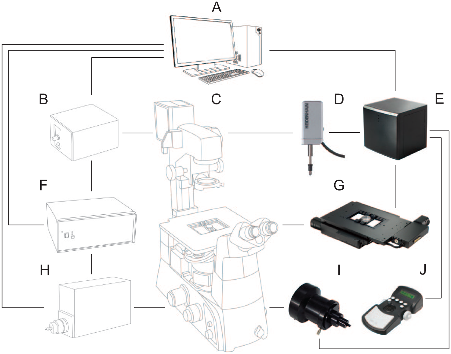
Illustration of the components for FLIM automation. Black lines show the connections between them. (A) Computer with Li-FLIM software package, including extensions to control the stage and focus drive. (B) TRiCAM CCD camera. (C) Inverted microscope. (D) Z encoder probe. (E) Proscan III controller. (F) LIFA control unit. (G) Proscan inverted stage. (H) Multi-LED, pulsed excitation light source. (I) Focus drive. (J) Proscan III joystick.

A regular computer with at least a 2.0 GHz processor and Windows XP (Microsoft) or later version of the operating system provides communication between all components of the automated FLIM system. The computer has the LI-FLIM software package version 1.2.25 (Lambert Instruments) installed and, in addition, the LI Prior Plugin v1.1 extension to control the stage and focus drive. LI-FLIM accesses the Proscan III controller using the software development kit that this controller has integrated and is then able to move both the stage and focus drive, taking the sample to a different position before the next image is acquired. LI-FLIM comes with automated features such as time-lapse measurements. For automated FLIM imaging, this is combined with moving of the stage to a new position. Before each new time point is measured, a change of position is inserted, so that each new time point corresponds to a different position of the sample. Once full integration of the components is achieved, all that is needed for FLIM automation is a protocol defining the list of positions, which depend on the type of sample that is going to be used.

Predefined Positioning Protocols for 96-Well and Microscope Slide Imaging

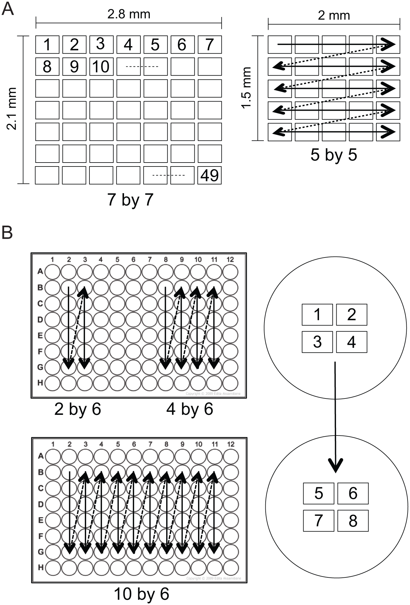
Two different types of positioning protocols have been created for FLIM automation, one to be used with conventional microscope slides ( Fig. 2A ) and the other for use with 96-well plates ( Fig. 2B ). Positioning protocols are basically a predefined list of coordinates X, Y, and Z, given in .txt format, that the LI Prior Plugin can load and use. In both cases, the user simply defines the starting point, and from there, the automated FLIM imaging will take control and make the acquisition without any human intervention.

Figure 2.

(A) Established positioning formats for conventional microscope slides. Left: 7 × 7 format showing the order of acquisition and image number assignment. The distances between images are 400 μm on the X axes and 300 μm on the Y axes. Right: 5 × 5 format showing the direction in which images are acquired. The order of image acquisition is analogous in these two formats. (B) Established positioning formats for 96-well plates. Left: 2 × 6, 4 × 6, and 10 × 6 formats showing the positioning direction. Right: Details of positioning within individual wells where four images are acquired inside each well. Note: Images are not to scale.

For microscope slides, we have realized two positioning formats, a 5 × 5 format and a 7 × 7 format ( Fig. 2A ), which are both in a grid layout in order to cover a larger area from the microscopic sample. After the image at the starting point is taken, the stage is shifted 400 μm to the left so that the field of view is that just to the right of the previous one. Here, a new image is acquired, and this is repeated for five or seven steps, depending on the format that was chosen. Then the stage is taken back to the starting X position and shifted 300 μm north in the Y direction, thus allowing imaging of the next row south of the first one. From this point, analogous movements are repeated until the entire 5 × 5 or 7 × 7 grid is imaged. (Details for order of images and positioning direction can be seen in Fig. 2A . Note that the sequence of events is analogous for both positioning protocols.)

For 96-well plates, three different protocols were developed, 2 × 6, 4 × 6, and 10 × 6 well formats ( Fig. 2B ). Each of these formats addresses six wells in the same column before moving to the next column to repeat the process, scanning 2, 4, or 10 columns, as the format name indicates. Moreover, within each individual well, images are acquired on four different positions in a gridlike pattern going from left to right and top to bottom and with the same spacing between images as described for the microscope slides ( Fig. 2B , right). After all four images are taken in one well, the stage moves to the next well to repeat this step.

Since our automation setup does not have an autofocus system, the default configuration in each of these protocols is for the focus control to keep the Z position constant at the position defined at the starting point by the user. For situations where either the microscope slides or the 96-well plates are not perfectly flat and straight, and the correct focus position (Z position) is not the same at every X and Y coordinate, we have created a simple focus compensation system. The focus compensation system calculates the Z position for every X and Y coordinate combination if the Z position of three of the four corner positions of the relevant sample area (typically coverslip corners of the slide or corner wells) is given. So assuming that the user has set the starting position to be the 0 focus position, then simply by checking the Z focus position at two other corners (actually, left bottom and right bottom corners), the compensation system will be able to calculate the focus position at all other intermediary X and Y positions. This focus compensation assumes that differences in the focus position are due to a tilt on the sample and calculates the focus at each coordinate X and Y by fitting a plane with a steady slope to the three corner positions that are given by the user. If changes in focus positions were due to irregularities on the surface of slides or 96-well plates, focus compensation would not be able to correct for this. Incorporation of an autofocus system could then provide a solution. All positioning protocols, focus compensation files, and a comprehensive user manual can be found for download as a zip-compressed folder appended to this manuscript as a supplementary file.

Display and Storage of Images and Lifetime Measurements

As automated spatial imaging is implemented via the time-lapse measurement option of the LI-FLIM software, images and lifetime measurements can be immediately displayed after each image is acquired. While the fluorescence lifetime is calculated per pixel and complete lifetime maps are automatically stored after a complete sequence of images is taken, we calculate the average of the complete field of view and a single result is given per FLIM image or location. Lifetime values can be directly exported as a table containing the frame/image number, the elapsed time from start until the moment when each image was acquired, the average lifetime of the whole field of view, the standard deviation, and the number of pixels used to calculate the lifetime. If specific results per pixel or per region of interest (ROI) are desired, these can be extracted by selecting them on the images and exporting the results table. User-defined intensity thresholds allow the exclusion of any of those pixels from the averaging that have either a too low or too high fluorescence signal from within the Li-FLIM software. Note that this FLIM automation setup does not keep a direct link between the lifetime data and the well position where it was acquired; the only label it has is the frame/image number. To overcome this limitation for data acquired in 96-well plates, we have created an external Excel file named “Plate Map.xlsx” (available in the zip-compressed folder appended to this manuscript as a supplementary file). Having documented the positioning protocol and the starting position, the user can create a plate map that will display each lifetime result color-coded at its position in the 96-well plate. The full sequence of images can also be saved in video format, which later can be read and quantified with any image processing data.

Performance Comparison of Automated and Manual FLIM Imaging

In order to test the performance of this FLIM automation system, the interaction between key players of the Ras/MAPK pathway, the oncoprotein Ras and its effector Raf, was studied. An effector typically requires binding to membrane-anchored Ras for its activation. Therefore, our FRET pair consisting of the mGFP-tagged Ras together with the mRFP-tagged Ras binding domain of C-Raf (RBD) not only provides an excellent test sample for FRET efficiency measurements, but also represents a very interesting target for further applications in chemogenomics. A comparison of fluorescence lifetimes determined in a manual versus an automated fashion from HEK293 EBNA cells transiently expressing mGFP-K-rasG12V alone (donor only) or mGFP-K-rasG12V and mRFP-RBD (FRET sample) is presented in Figure 3 . The exact same microscope slide samples were imaged and quantified with both methods. For manual FLIM, more than 250 cells were imaged, with the user individually adjusting the position and focus in every field of view and taking approximately 4 h to measure and extract the lifetime values from each individual cell. Automated FLIM measurements in a 7 × 7 format provide one lifetime value per field of view (49 fields of view with ~8 cells in each), and there is no need for user intervention besides the initial setting of focus and starting coordinates. Imaging and lifetime calculation takes less than 4 min, in this case representing a time saving by a factor of 60. Our results show that the average and median lifetimes from manual and automated FLIM measurements are slightly offset from each other, but are very comparable ( Fig. 3 ). Importantly, also improvements on the standard error of the mean are observed in automation measurements due to the higher number of cells that were acquired and to the fact that every lifetime recorded is given for a whole field of view (5–10 cells) and not for individual cells, reducing the effect from cell-to-cell variation.

Figure 3.

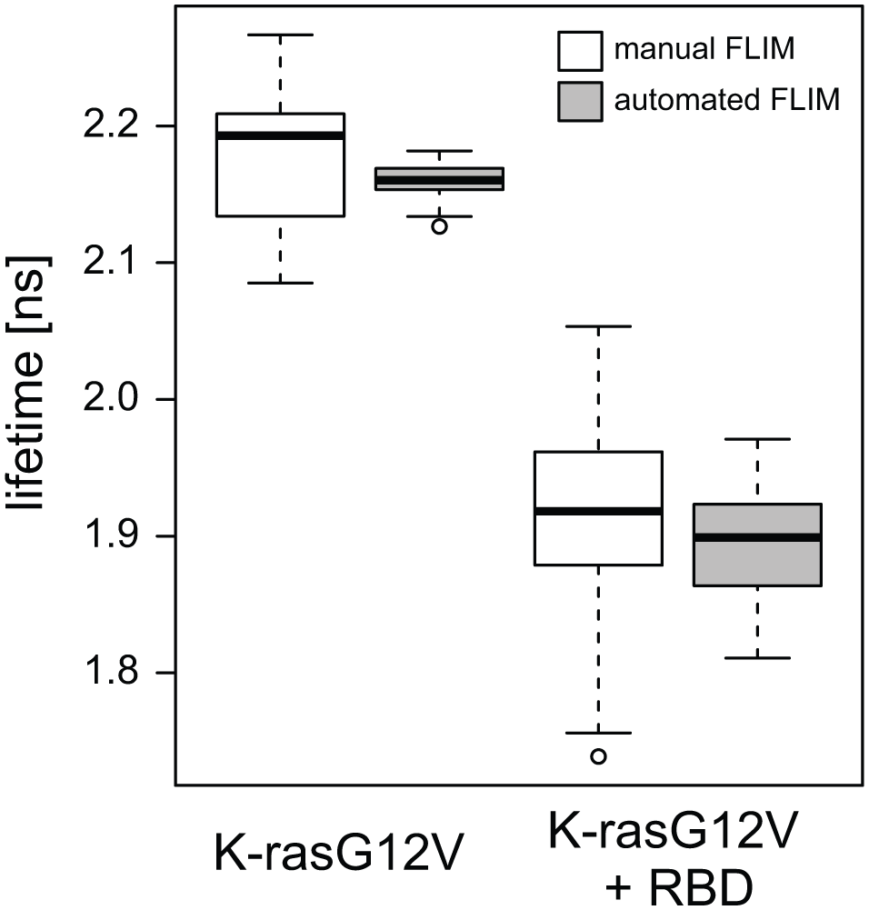
Fluorescence lifetimes of HEK293 EBNA cells transiently expressing mGFP-K-rasG12V alone (donor only) or mGFP-K-rasG12V and mRFP-RBD (FRET sample). Results obtained with manual FLIM (3 biological repeats, ~250 imaged cells per sample, ~4 h acquisition and analysis time) are compared to those obtained with automated FLIM (1 biological repeat, ~ 500 imaged cells per sample, ~4 min acquisition and analysis time). Imaging was performed on microscope slides and, in the case of automated FLIM, using a 7 × 7 scan format. Boxplots show the distribution of the data with the median of the data (bold line), the first and the third quartiles (lower and upper boxes), Q3 + 1.5 × interquartile range (upper whisker), Q1 – 1.5 × interquartile range (lower whisker), and the outliers (circles).

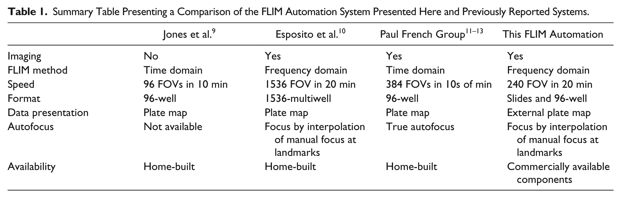
A comparison between the FLIM automation system presented here and those systems created in the past by others can be found in Table 1 .

Table 1.

Summary Table Presenting a Comparison of the FLIM Automation System Presented Here and Previously Reported Systems.

	Jones et al.⁹	Esposito et al.¹⁰	Paul French Group^11–13	This FLIM Automation
Imaging	No	Yes	Yes	Yes
FLIM method	Time domain	Frequency domain	Time domain	Frequency domain
Speed	96 FOVs in 10 min	1536 FOV in 20 min	384 FOVs in 10s of min	240 FOV in 20 min
Format	96-well	1536-multiwell	96-well	Slides and 96-well
Data presentation	Plate map	Plate map	Plate map	External plate map
Autofocus	Not available	Focus by interpolation of manual focus at landmarks	True autofocus	Focus by interpolation of manual focus at landmarks
Availability	Home-built	Home-built	Home-built	Commercially available components

Automated FLIM Imaging of a Dose–Response Curve in a 96-Well Plate

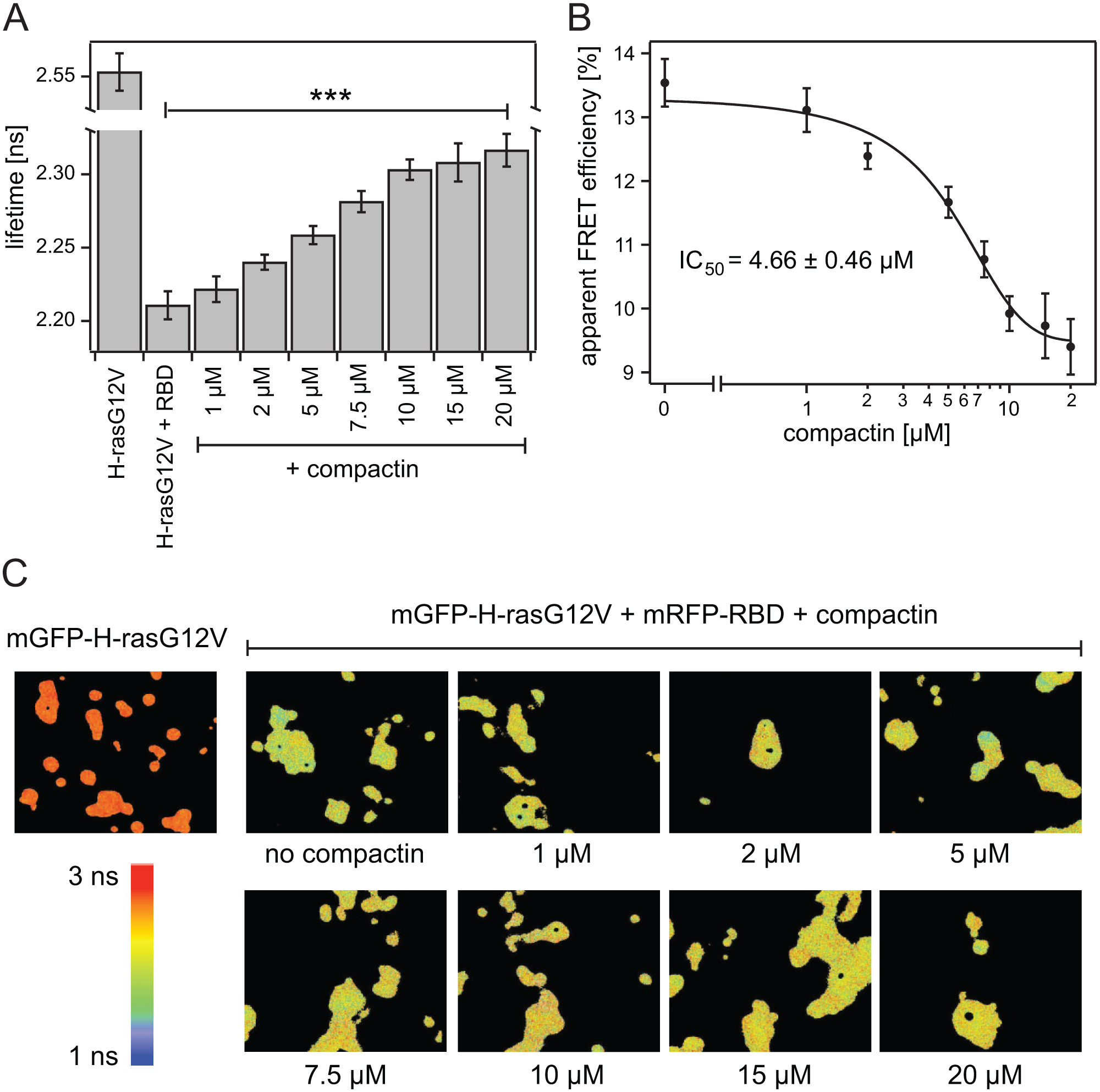
As the main goal of an automated FLIM system is to perform fast measurements on large numbers of samples with high precision, this system was further tested by establishing a dose–response curve of the effect that the drug compactin, a statin, has on the recruitment of the effector Raf to Ras. It is well known that upon treatment with the drug compactin, Ras changes its localization from membrane bound to a cytoplasmic localization, and therefore the recruitment of its effector Raf will be disrupted.¹⁷ Ninety-six-well plates containing HEK293 EBNA cells transiently expressing mGFP-H-rasG12V alone (donor only) or mGFP-H-rasG12V and mRFP-RBD (FRET samples) were treated with different concentrations of compactin for 24 h before FLIM images were acquired. Only the inner 60 wells of the 96-well plate were used, providing 6 wells for each condition or treatment. Data acquisition was done on the 6 × 10 format (with four images per well), taking just under 20 min. Lifetime values show a highly significant difference (p = 2 × 10⁻¹⁶) in lifetime from the donor-only sample to all the FRET samples, evidencing the good FRET efficiency ( Fig. 4A ). Treatment with increasing concentrations of compactin caused a gradual and small increase of the fluorescence lifetime that corresponds to the loss of FRET caused by the relocalization of Ras to the cytoplasm ( Fig. 4A , C ). Lifetime values were converted into apparent FRET efficiency values, and this data set was used to calculate a dose–response curve for the loss of binding between Ras and its effector Raf upon treatment with compactin in cells ( Fig. 4B ). The IC₅₀ value obtained for compactin (also known as mevastatin) was 4.66 ± 0.66 μM and is in good agreement with published values from similar studies.^18,19 These results show that although the changes in lifetime might be small from one concentration to another ( Fig. 4C ), they can be precisely quantified in a short amount of time. The large number of possible samples and relatively high speed provide a basis for FLIM-FRET-based medium- to high-throughput projects, such as encountered in secondary and orthogonal validation assays after large screening campaigns.

Figure 4.

(A) Fluorescence lifetimes of HEK293 EBNA cells transiently expressing mGFP-H-rasG12V alone (donor only) or mGFP-H-rasG12V and mRFP-RBD (FRET samples) were treated with different concentrations of compactin, which prevents H-rasG12V membrane anchorage and thus efficient recruitment of the RBD,¹⁷ only to H-Ras organized in nanoscale clusters in the membrane. Imaging was performed in a conventional 96-well plate using the 10 × 6 format and with 6 wells per condition (4 images per well, 24 images per condition, 216 images total). Bars correspond to the average lifetime ± SEM. (B) Apparent FRET efficiency of FRET samples presented in A as a function of the compactin concentration. Data points correspond to the average apparent FRET efficiency ± SEM. A sigmoidal fit was added to establish the dose–response curve and calculate the IC₅₀ value. (C) Arbitrarily selected sample images from samples in A showing the fluorescence lifetime calculated per pixel of individual cells.

Conclusions

We presented a microscopy setup for automated FLIM-FRET imaging that is entirely based on commercial components, thus making it accessible to many laboratories. Using predefined positioning protocols, the system can acquire images from microscopic slides or 96-well plates and precisely calculate the fluorescence lifetimes from samples in a matter of minutes without any user supervision. The much larger number of samples that can be processed compared to manual data acquisition makes this system suitable for high-content or medium- to high-throughput imaging with broad applicability in chemogenomics projects.

Footnotes

Acknowledgements

We would like to acknowledge Maja Šolman (Turku Centre for Biotechnology, Turku, Finland) for help with acquisition of manual FLIM data and Johan Herz (Lambert Instruments, Groningen, Netherlands) for help with software customization and hardware integration.

Supplementary material for this article is available on the Journal of Laboratory Automation Web site at .

Declaration of Conflicting Interests

The authors declared no potential conflicts of interest with respect to the research, authorship, and/or publication of this article.

Funding

The authors disclosed receipt of the following financial support for the research, authorship, and/or publication of this article: This work was supported by grants to D.A. from the Academy of Finland Fellowship (grant numbers: 252381, 256440, 281497) and MC-IRG (NANODYGP) (grant number: 268271).

References

Tramier

M. M.

Piolot

T. T.

Gautier

I. I.

. Homo-FRET versus Hetero-FRET to Probe Homodimers in Living Cells. Meth. Enzymol. 2002, 360, 580–597.

Jares-Erijman

E. A.

Jovin

T. M.

FRET Imaging. Nat. Biotechnol. 2003, 21, 1387–1395.

Jares-Erijman

E. A.

Jovin

T. M.

Imaging Molecular Interactions in Living Cells by FRET Microscopy. Curr. Opin. Chem. Biol. 2006, 10, 409–416.

Padilla-Parra

Tramier

FRET Microscopy in the Living Cell: Different Approaches, Strengths and Weaknesses. Bioessays 2012, 34, 369–376.

Matthews

D. R.

Fruhwirth

G. O.

Weitsman

. A Multi-Functional Imaging Approach to High-Content Protein Interaction Screening. PLoS One 2011, 7, e33231–e33231.

Köhnke

Schmitt

Ariotti

. Design and Application of In Vivo FRET Biosensors to Identify Protein Prenylation and Nanoclustering Inhibitors. Chem. Biol. 2012, 19, 866–874.

Najumudeen

A. K.

Köhnke

Šolman

. Cellular FRET-Biosensors to Detect Membrane Targeting Inhibitors of N-Myristoylated Proteins. PLoS One 2013, 8, e66425.

Najumudeen

A. K.

Guzmán

Posada

I. M. D.

. Rab-NANOPS: FRET Biosensors for Rab Membrane Nanoclustering and Prenylation Detection in Mammalian Cells. Methods Mol. Biol. 2015, 1298, 29–45.

Jones

P. B.

Herl

Berezovska

. Time-Domain Fluorescent Plate Reader for Cell Based Protein-Protein Interaction and Protein Conformation Assays. J. Biomed. Opt. 2006, 11, 054024.

10.

Esposito

Dohm

C. P.

Bähr

. Unsupervised Fluorescence Lifetime Imaging Microscopy for High Content and High Throughput Screening. Mol. Cell. Proteomics 2007, 6, 1446–1454.

11.

Talbot

C. B.

McGinty

Grant

D. M.

. High Speed Unsupervised Fluorescence Lifetime Imaging Confocal Multiwell Plate Reader for High Content Analysis. J. Biophotonics 2008, 1, 514–521.

12.

Kumar

Alibhai

Margineanu

. FLIM FRET Technology for Drug Discovery: Automated Multiwell-Plate High-Content Analysis, Multiplexed Readouts and Application In Situ. Chemphyschem 2011, 12, 609–626.

13.

Alibhai

Kelly

D. J.

Warren

. Automated Fluorescence Lifetime Imaging Plate Reader and Its Application to Förster Resonant Energy Transfer Readout of Gag Protein Aggregation. J. Biophotonics 2013, 6, 398–408.

14.

Abankwa

Hanzal-Bayer

Ariotti

. A Novel Switch Region Regulates H-Ras Membrane Orientation and Signal Output. EMBO J. 2008, 27, 727–735.

15.

Abankwa

Gorfe

A. A.

Inder

. Ras Membrane Orientation and Nanodomain Localization Generate Isoform Diversity. Proc. Natl. Acad. Sci. U.S.A. 2010, 107, 1130–1135.

16.

Majoul

Jia

Duden

Practical Fluorescence Resonance Energy Transfer or Molecular Nanobioscopy of Living Cells. In Handbook of Biological Confocal Microscopy; Pawley

J. V.

, Ed., Springer: Berlin, 2006; 3rd ed., pp 788–808.

17.

Guzmán

Šolman

Ligabue

. The Efficacy of Raf Kinase Recruitment to the GTPase H-Ras Depends on H-Ras Membrane Conformer-Specific Nanoclustering. J. Biol. Chem. 2014, 289, 9519–9533.

18.

Glynn

S. A.

O’Sullivan

Eustace

A. J.

. The 3-Hydroxy-3-Methylglutaryl-Coenzyme A Reductase Inhibitors, Simvastatin, Lovastatin and Mevastatin Inhibit Proliferation and Invasion of Melanoma Cells. BMC Cancer 2008, 8, 9.

19.

Evangelopoulos

M. E.

Weis

Krüttgen

Mevastatin-Induced Neurite Outgrowth of Neuroblastoma Cells via Activation of EGFR. J. Neurosci. Res. 2009, 87, 2138–2144.

Supplementary Material

Please find the following supplemental material available below.

For Open Access articles published under a Creative Commons License, all supplemental material carries the same license as the article it is associated with.

For non-Open Access articles published, all supplemental material carries a non-exclusive license, and permission requests for re-use of supplemental material or any part of supplemental material shall be sent directly to the copyright owner as specified in the copyright notice associated with the article.

5.55 MB

0.00 MB

Automated High-Throughput Fluorescence Lifetime Imaging Microscopy to Detect Protein–Protein Interactions