Sage Journals: Discover world-class research

Abstract

Study Design

Retrospective observational study.

Objectives

Scoliosis is commonly observed in adolescents, with a world0wide prevalence of 0.5%. It is prone to be overlooked by parents during its early stages, as it often lacks overt characteristics. As a result, many individuals are not aware that they may have scoliosis until the symptoms become quite severe, significantly affecting the physical and mental well-being of patients. Traditional screening methods for scoliosis demand significant physician effort and require unnecessary radiography exposure; thus, implementing large-scale screening is challenging. The application of deep learning algorithms has the potential to reduce unnecessary radiation risks as well as the costs of scoliosis screening.

Methods

The data of 247 scoliosis patients observed between 2008 and 2021 were used for training. The dataset included frontal, lateral, and back upright images as well as X-ray images obtained during the same period. We proposed and validated deep learning algorithms for automated scoliosis screening using upright back images. The overall process involved the localization of the back region of interest (ROI), spinal region segmentation, and Cobb angle measurements.

Results

The results indicated that the accuracy of the Cobb angle measurement was superior to that of the traditional human visual recognition method, providing a concise and convenient scoliosis screening capability without causing any harm to the human body.

Conclusions

The method was automated, accurate, concise, and convenient. It is potentially applicable to a wide range of screening methods for the detection of early scoliosis.

Keywords

scoliosis screening deep learning back images spinal segmentation cobb angle measurement

Introduction

Scoliosis is an abnormal sideways curve of the spine. It may carry a rotation of the vertebrae, and the curvature may be multi-directional. It is not a specific disorder, but a series of diseases with similar conditions. There are many different forms or causes of scoliosis, eg, neuromuscular, congenital, syndromic or even cicatricial scoliosis.¹ The majority of all scoliosis (80%–90%) are referred to as idiopathic scoliosis when no underlying disease can be found.² Scoliosis is more common in adolescents because it tend to worsen during periods of increased growth without intervention, resulting in increased curvature and also trunk deformity. It is not easily detected because it does not have distinctive features in earlier occurrences. As a result, by the time scoliosis is identified, many patients have scoliosis deformities that are so severe that they cannot be remedied by orthopedic or other means and can only be treated surgically, which has a tremendous physical and psychological impact on the patient.^2–4

There are three main methods used for the screening of scoliosis. These are physical examinations, X-ray testing, and Surface topography detectors.³ X-Ray testing is the most accurate, but is expensive. Therefore, most diagnoses use a combination of a physical examination and radiographic testing, based on a physical examination assessment before confirmation. This approach solves the problems of screening resources and subject apprehension, but there is a risk of a diagnostic error because the physical examination is a manual assessment.

With the rapid development of technology, computer-aided diagnosis (CAD) has successfully been applied to diagnose various diseases such as lung and skin cancers.⁴ Computer-aided diagnosis has become an essential topic in the medical imaging discipline and physicians can use it to produce rapid diagnostic decisions. The high accuracy and convenience of computer-aided diagnosis have contributed to the development of intelligent medicine. An increasing number of researchers are studying the application of computer-aided diagnosis with regard to pathological images.^5,6

Many scoliosis screenings are conducted using X-rays, but recent studies have used back photographs to enable scoliosis screening.⁷ Back image data are easily available and can be taken with a cell phone, avoiding exposure to radiation from X-rays. Regarding the image data selection, images of the upright state of the back are abundant and accessible. The Cobb angle is the gold standard for a scoliosis diagnosis; Cobb angle measurements after segmenting the spine are more reliable than image classification. In this study, we designed a deep learning algorithm to calculate the Cobb angle of a spine from an upright image of the back to determine whether the subject had scoliosis. Our aim was to achieve the fast, simple, effective, and risk-free intelligent screening of scoliosis.

Materials and Methods

The primary research in this paper centered on the localization of the region of interest in back upright images for the detection of scoliosis. For localization, we evaluated four models based on the YOLOv5 architecture. Finally, we selected the YOLOv5x model for the localization of the back region. To detect scoliosis, we measured the Cobb angle of the spine, considering the importance of the Cobb angle in diagnosing scoliosis. We used the U-Net network with the residual module of ResNet to achieve segmentation of the spine in the back region. We then used a least squares polynomial fit to represent the segmented spine as a function of the curve, automatically measuring the Cobb angle of the spine by calculating the slope of the tangent line at the second-order derivative of the curve at 0 as the Cobb angle of the spine.

The overall technical approach is illustrated in Figure 1. First, spinal images were annotated and used to train the YOLOv5 model. The parameters and architecture of the model were fine-tuned until optimal performance was achieved. Second, an improved U-Net network was used to automatically segment the segmented spinal images, resulting in the shape curves of the spine. Finally, the spinal curves were fitted using the least squares method, allowing for the automated calculation of the Cobb angle.

Figure 1.

Overall technical approach.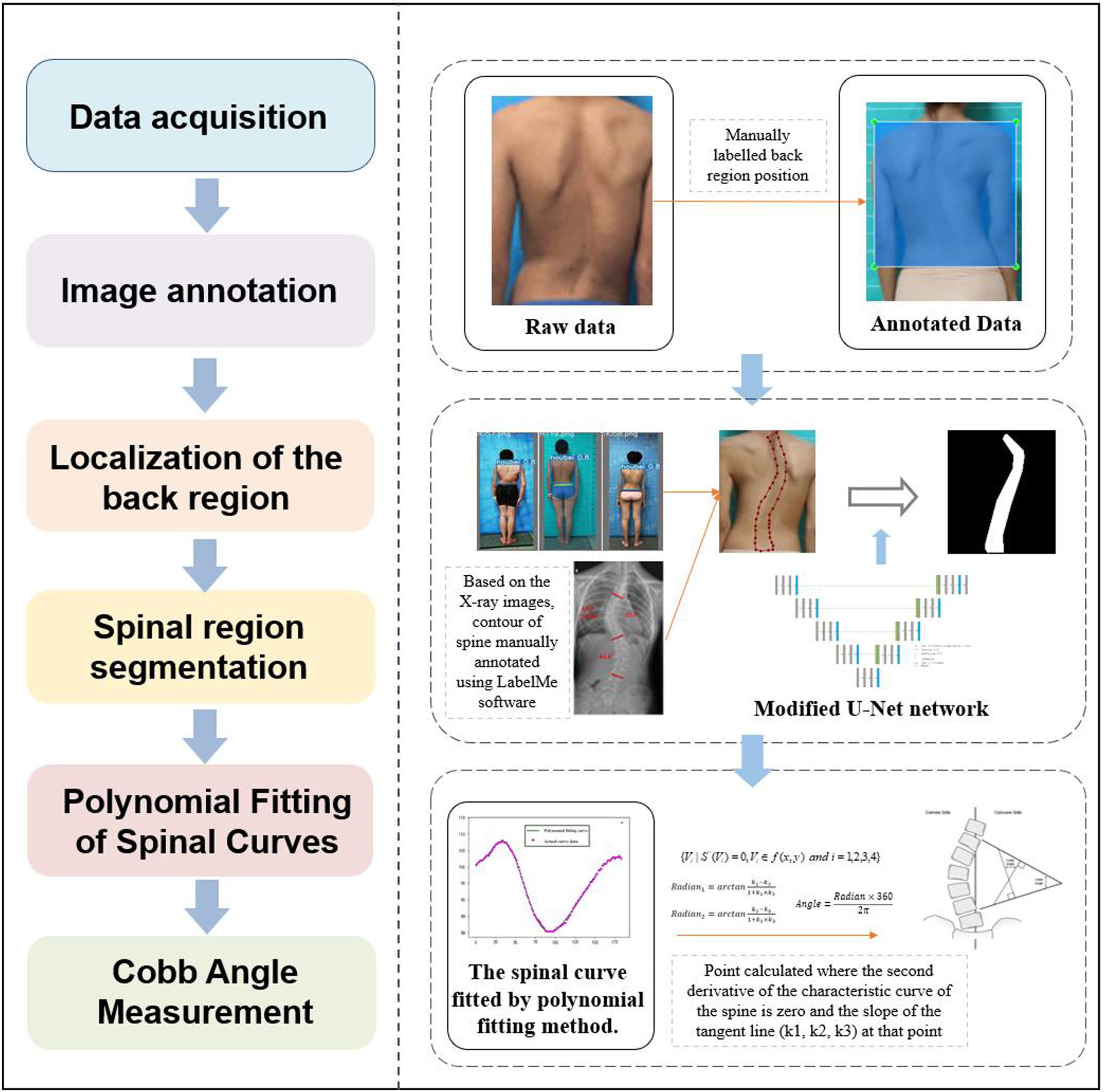

Image Localization

The device used in this study was a Dell XPS 9830 computer (Intel (R) Core (TM) i7-8700 CPU, 3.20 GHz, and 16 GB RAM; NVIDIA GeForce GTX 1070 GPU; 6 GB VRAM, and 64-bit operating system) running Windows 11. We established a virtual environment using Anaconda and built a PyTorch deep learning framework. The algorithm for object detection and localization based on the YOLOv5 model was developed using Python language programs, which used various libraries (including CUDA, CuDNN, and OpenCV). These tools were used to perform the training and testing.

Data Acquisition

The dataset used in this study was obtained from the Affiliated Beijing Chaoyang Hospital of Capital Medical University from scoliosis patients observed between 2008 and 2021. The data of 247 patients were used for training. The dataset included frontal, lateral, and back upright images as well as X-ray images obtained during the same period.

Annotation Process

The labels for the YOLOv5 training dataset were primarily created using labeling software and an open-source graphical image annotation tool written in Python,⁸ using Qt as its image interface. The tool adhered to the PASCAL VOC format of the ImageNet dataset for storing labeled data, resulting in files with an xml format. YOLOv5 uses the txt format for labels; it requires a five-item data representation to represent the position of each labeled box, including the target species, the center point x and y values, the width, and the height of the labeled box. Therefore, all annotated xml files were converted to files with a. txt format before dividing the raw data and corresponding labels into training and validation sets at a ratio of 4:1.

Network Training

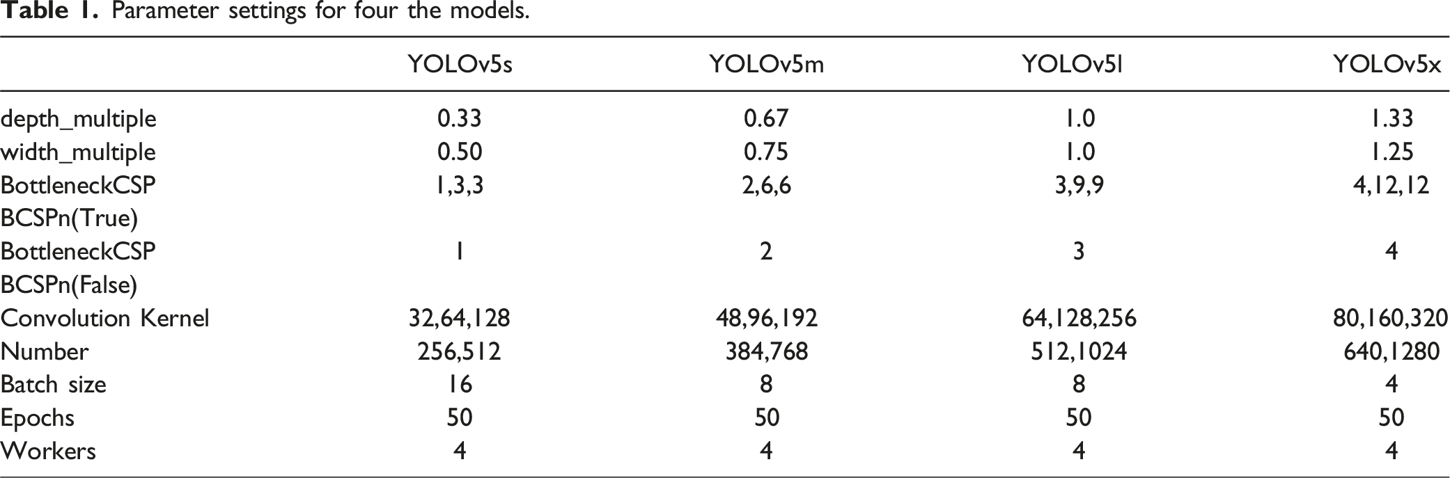
We trained our dataset using YOLOv5s, YOLOv5m, YOLOv5l, and YOLOv5x models. We evaluated their performance to identify the optimal model. YOLOv5 incorporates channel and layer control factors similar to EfficientNet. These are controlled by two parameters, depth_multiple and width_multiple, to adjust the depth and width of the network, respectively. The number of BottleneckCSPs was specifically adjusted to control the depth of the network. The number of convolutional kernels was adjusted to control the width.

Each model was trained with its corresponding weight file. The default value for the parameter of the YOLOv5 workers was 8; however, we observed that setting it to 4 improved the GPU utilization efficiency and reduced the memory requirements. We determined the optimal number of epochs through multiple tests for each network. Due to limitations imposed by the training platform and varying model complexities, different batch sizes were used for each model. The parameter settings are shown in Table 1.

Table 1.

Parameter settings for four the models.

	YOLOv5s	YOLOv5m	YOLOv5l	YOLOv5x
depth_multiple	0.33	0.67	1.0	1.33
width_multiple	0.50	0.75	1.0	1.25
BottleneckCSP	1,3,3	2,6,6	3,9,9	4,12,12
BCSPn(True)	1,3,3	2,6,6	3,9,9	4,12,12
BottleneckCSP	1	2	3	4
BCSPn(False)	1	2	3	4
Convolution Kernel	32,64,128	48,96,192	64,128,256	80,160,320
Number	256,512	384,768	512,1024	640,1280
Batch size	16	8	8	4
Epochs	50	50	50	50
Workers	4	4	4	4

Evaluation Metrics for Network Performance

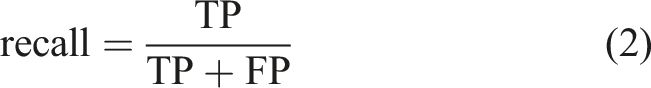
In this study, we used several evaluation metrics to determine the effectiveness of the YOLOv5 model; namely, precision, recall, PR curve, AP, mAP, and F1 score. Precision and recall evaluated the accuracy and completeness of the predictions of the model, respectively. The calculations of precision and recall were based on the results of four fundamental indicators. These were true-positive (TP), false-negative (FN), false-positive (FP), and true-negative (TN). The formulae for these indicators can be expressed using Equations (1) and (2).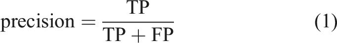

precision = \frac{TP}{TP + FP}

(1)

recall = \frac{TP}{TP + FP}

(2)

The F1 score is known as the balanced F Score, which is the harmonic mean of precision and recall (equation (3)).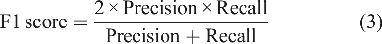

F 1 score = \frac{2 \times Precision \times Recall}{Precision + Recall}

(3)

The F1 score ranges from 0 to 1. Values closer to 1 indicate an improved model performance; conversely, values closer to 0 indicate a poorer model performance.

In addition to the balanced F1 Score, PR curves can provide a more intuitive analysis of the performance of a model through visualization. When determining precision, assigning a threshold value to the sample is required to determine whether the predicted result is a true positive. Different threshold values will result in different precision and recall values. The PR curve depicts the relationship between precision and recall at different threshold values. Each threshold value corresponds with a point on the PR curve.

Automatic Spinal Segmentation Algorithm Construction

Network Architecture and Loss Function Design

Given the relative scarcity of available data for this study, we opted to use the U-Net ⁹ network to segment the spinal region in the back area to describe the overall curvature of the spine. CNNs are commonly used in image recognition tasks; however, deeper networks often suffer from performance degradation and longer training times. A solution to this problem is the ResNet. ResNet ^10-12 introduced the concept of shortcut connections, which skip one or multiple layers and directly add the input to a layer below. ResNet can be represented by equation (4).

H (x) = x + F (x)

(4)

H (x)

where

H (x)

represents the result of the bottom-level mapping,

x

denotes the input of the network, and

F (x)

signifies the output of the hidden layer calculation in the intermediate stage of the network.

The loss function of a network is calculated using a combination of the cross-entropy loss function with weights and per-pixel SoftMax values on the final feature map. Similar to linear regression, SoftMax regression¹³ also linearly combines the input features and weights. However, the difference lies in the fact that the number of output results from SoftMax is determined by the number of categories in the labels. The SoftMax function is shown in equation (5).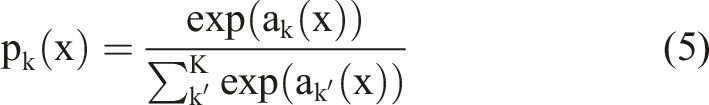

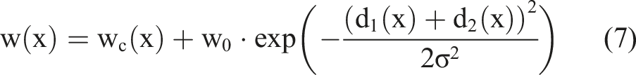
p_{k} (x) = \frac{\exp (a_{k} (x))}{\sum_{k^{'}}^{K} \exp (a_{k^{'}} (x))}

(5)

In this equation,

a_{k} (x)

refers to the activation value of pixel position x in the k-th feature channel and

p_{k} (x)

is an approximate maximum function. The calculation method for cross-entropy can be derived based on

p_{k} (x)

as follows:

E = \sum_{X \in Ω} w (x) \log (p_{l_{(x)}} (x))

(6)

In this equation,

l

represents the true label for each pixel and

w

denotes the weight added to each pixel. The specific formula is as follows:

w (x) = w_{c} (x) + w_{0} \cdot \exp (- \frac{{(d_{1} (x) + d_{2} (x))}^{2}}{2 σ^{2}})

(7)

Equation (7) is a learning method to calculate the normal distribution. Here, $w_{c} (x)$ represents the compensation of different pixel frequencies for each class in the ground truth segmentation, which is calculated in advance. The variables $d 1$ and $d 2$ represent the distances to the nearest and second-nearest cell boundaries, respectively.

Data Preprocessing

Accurately identifying the spine in back images can be challenging; therefore, we used radiographs to aid annotation. To ensure precise labeling, we employed a dense labeling strategy. This allowed us to accurately depict the closed area and produce images with smooth labeling. The Cobb angles of the spine were measured by determining the upper- and lower-end vertebrae of the spine on the radiographic images.¹⁴ Their Cobb angles were measured using a protractor. The angles of all spine vertebrae extensions were separately measured to measure the Cobb angles of the spine. As this system did not distinguish between thoracic and lumbar curvatures in the measurements, the maximum value of thoracic and lumbar curvatures was used as the result for all control data.

Based on the objectives of our algorithm and taking into consideration practical application scenarios,^15-18 data augmentation was performed on our dataset using Gaussian noise injections, image flipping, and brightness adjustments. These operations were applied to account for various factors that could affect the accuracy of the back upright images; for example, differences in pixel resolutions, the angles of capture, and variations in the lighting conditions of rooms.

Network Training and Performance Analysis

After conducting preliminary testing, we determined that setting the number of epochs to 50 produced the most effective training results because overfitting became more pronounced beyond this threshold. The batch size parameter was set to 16, the start frame was set to 16, and the drop rate was set to 0.5. To determine the optimal learning rate, the model was trained with four different learning rates; ie, 0.002, 0.001, 0.0005, and 0.00025.

Polynomial Fitting of Spinal Curves Based on Least Squares Method

In this study, we used the method of polynomial fitting based on the least squares method^19-21 to fit the segmented spinal images to curves. The error between the original function and the fitted curve could be represented in the form of equation (8).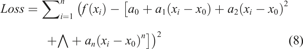

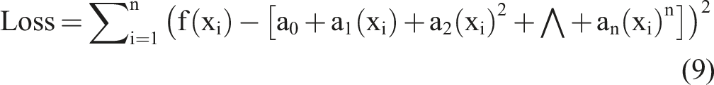
L o s s = \sum_{i = 1}^{n} {(f (x_{i}) - [a_{0} + a_{1} (x_{i} - x_{0}) + a_{2} {(x_{i} - x_{0})}^{2} + \land + a_{n} {(x_{i} - x_{0})}^{n}])}^{2}

(8)

When

x_{0}

equaled zero, the least squares error could be represented using equation (9).

Loss = \sum_{i = 1}^{n} {(f (x_{i}) - [a_{0} + a_{1} (x_{i}) + a_{2} {(x_{i})}^{2} + \land + a_{n} {(x_{i})}^{n}])}^{2}

(9)

To achieve the optimal objective function, we took a partial derivative of equation (9) and set it to equal zero as follows: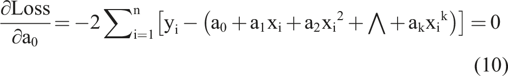

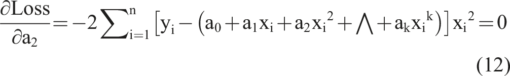
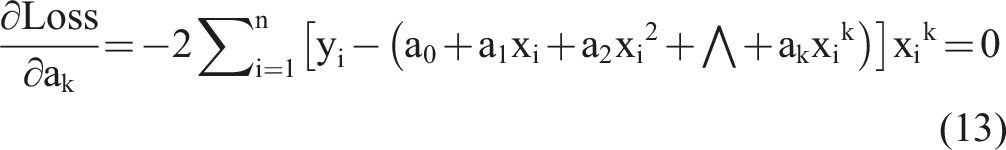
\frac{\partial Loss}{\partial a_{0}} = - 2 \sum_{i = 1}^{n} [y_{i} - (a_{0} + a_{1} x_{i} + a_{2} {x_{i}}^{2} + \land + a_{k} {x_{i}}^{k})] = 0

(10)

\frac{\partial Loss}{\partial a_{1}} = - 2 \sum_{i = 1}^{n} [y_{i} - (a_{0} + a_{1} x_{i} + a_{2} {x_{i}}^{2} + \land + a_{k} {x_{i}}^{k})] x_{i} = 0

(11)

\frac{\partial Loss}{\partial a_{2}} = - 2 \sum_{i = 1}^{n} [y_{i} - (a_{0} + a_{1} x_{i} + a_{2} {x_{i}}^{2} + \land + a_{k} {x_{i}}^{k})] {x_{i}}^{2} = 0

(12)

\dots

\frac{\partial Loss}{\partial a_{k}} = - 2 \sum_{i = 1}^{n} [y_{i} - (a_{0} + a_{1} x_{i} + a_{2} {x_{i}}^{2} + \land + a_{k} {x_{i}}^{k})] {x_{i}}^{k} = 0

(13)

Based on the k equations above, we could solve all unknown coefficients by following the approach of solving a system of linear equations using linear algebra, finding the optimal solution where the partial derivatives were minimized. We simplified the k equations, with the partial derivatives equaling zero, as follows: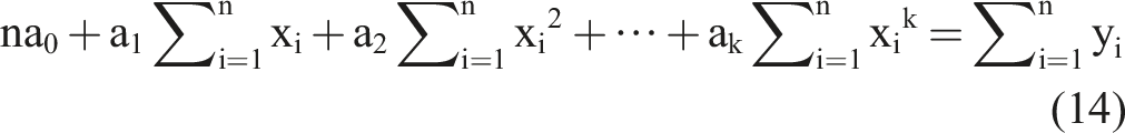

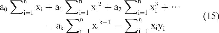
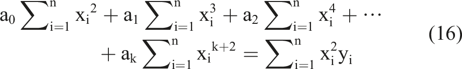
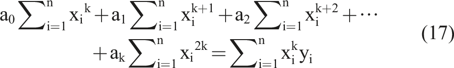
n a_{0} + a_{1} \sum_{i = 1}^{n} x_{i} + a_{2} \sum_{i = 1}^{n} {x_{i}}^{2} + \dots + a_{k} \sum_{i = 1}^{n} {x_{i}}^{k} = \sum_{i = 1}^{n} y_{i}

(14)

a_{0} \sum_{i = 1}^{n} x_{i} + a_{1} \sum_{i = 1}^{n} {x_{i}}^{2} + a_{2} \sum_{i = 1}^{n} x_{i}^{3} + \dots + a_{k} \sum_{i = 1}^{n} {x_{i}}^{k + 1} = \sum_{i = 1}^{n} {x_{i} y}_{i}

(15)

a_{0} \sum_{i = 1}^{n} {x_{i}}^{2} + a_{1} \sum_{i = 1}^{n} x_{i}^{3} + a_{2} \sum_{i = 1}^{n} x_{i}^{4} + \dots + a_{k} \sum_{i = 1}^{n} {x_{i}}^{k + 2} = \sum_{i = 1}^{n} {x_{i}^{2} y}_{i}

(16)

\dots

a_{0} \sum_{i = 1}^{n} {x_{i}}^{k} + a_{1} \sum_{i = 1}^{n} x_{i}^{k + 1} + a_{2} \sum_{i = 1}^{n} x_{i}^{k + 2} + \dots + a_{k} \sum_{i = 1}^{n} {x_{i}}^{2 k} = \sum_{i = 1}^{n} {x_{i}^{k} y}_{i}

(17)

By observing the k equations above, we observed that they could be regarded as a matrix multiplication. The matrix representation of equation (18) contains terms that appeared in all equations.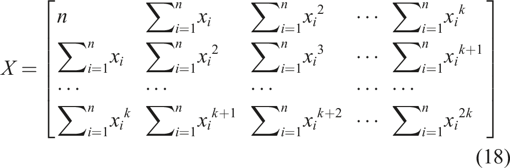

X = [\begin{array}{l} n & \sum_{i = 1}^{n} x_{i} & \sum_{i = 1}^{n} {x_{i}}^{2} & \cdot \cdot \cdot & \sum_{i = 1}^{n} {x_{i}}^{k} \\ \sum_{i = 1}^{n} x_{i} & \sum_{i = 1}^{n} {x_{i}}^{2} & \sum_{i = 1}^{n} {x_{i}}^{3} & \cdot \cdot \cdot & \sum_{i = 1}^{n} {x_{i}}^{k + 1} \\ \cdot \cdot \cdot & \cdot \cdot \cdot & \cdot \cdot \cdot & \cdot \cdot \cdot & \cdot \cdot \cdot \\ \sum_{i = 1}^{n} {x_{i}}^{k} & \sum_{i = 1}^{n} {x_{i}}^{k + 1} & \sum_{i = 1}^{n} {x_{i}}^{k + 2} & \cdot \cdot \cdot & \sum_{i = 1}^{n} {x_{i}}^{2 k} \end{array}]

(18)

The first k coefficients before 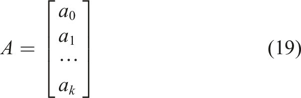$x$ are represented by matrix $A$ in equation (19).

A = [\begin{array}{l} a_{0} \\ a_{1} \\ \dots \\ a_{k} \end{array}]

(19)

The coefficients containing 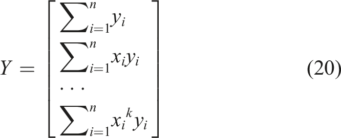$y$ are represented by matrix $Y$ in equation (20).

Y = [\begin{array}{l} \sum_{i = 1}^{n} y_{i} \\ \sum_{i = 1}^{n} x_{i} y_{i} \\ \cdot \cdot \cdot \\ \sum_{i = 1}^{n} {x_{i}}^{k} y_{i} \end{array}]

(20)

Thus, the initial k equations could be expressed in the form of equation (21).

X A = Y

(21)

From Equations (18) and (20), we observed that matrices $X$ and $Y$ did not contain any unknowns and matrix $A$ only contained the polynomial coefficients of $y$ . Therefore, the final problem was reduced by solving the linear equation system $X A = Y$ using Gaussian elimination ²² to obtain the coefficient matrix $A$ .

For the coefficients of the used polynomials, the number of terms varied across different vertebral data. We evaluated the choice of polynomial degree based on the sum of squared errors obtained from the least squares fitting process. For each vertebral curve, we set polynomial degrees from 7 to 11 and computed a fitted curve for each degree. By comparing the sum of squared errors of these curves, we selected the curve with the smallest error sum as the fitting curve for that vertebral curve.

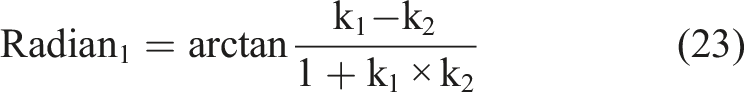
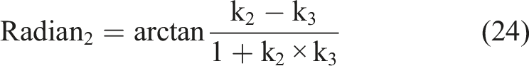
Cobb Angle Automated Measurement

According to the definition of the Cobb angle measurement, the Cobb angle is the angle between the tangents at the upper and lower vertebrae positions on the spinal curve. The upper and lower vertebrae can also be understood as the positions where the second-order derivative of the spinal curve is zero. Therefore, the measurement of the Cobb angle can be transformed into calculating the tangent angle at the position where the second-order derivative of the spinal curve is zero. By setting the spinal curve equation as $f (x, y)$ and applying equation (22), we could obtain the point where the second-order derivative was zero and calculate the tangent and the value of the Cobb angle.

{V_{i} | S^{″} (V_{i}) = 0, V_{i} \in f (x, y) a n d i = 1, 2, 3, 4}

(22)

In practice, deriving the spinal curve resulted in a slope curve of the curve. By acquiring a second derivative on the slope curve, we could obtain the extreme points of the slope curve (

(x_{1}, y_{1})

(x_{2}, y_{2})

, and

(x_{3}, y_{3})

) and the slope of the tangent lines (

k 1

k 2

, and

k 3

). Using Equations (23) and (24), we could calculate the Cobb angle in radians and convert it into the desired angle using equation (25).

Radia n_{1} = \arctan \frac{k_{1} {- k}_{2}}{1 + k_{1} \times k_{2}}

(23)

Radia n_{2} = \arctan \frac{k_{2} - k_{3}}{1 + k_{2} \times k_{3}}

(24)

Angle = \frac{Radian \times 360}{2 π}

(25)

Results

Localization Results of the Back Region

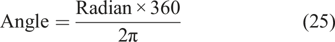
Regarding the loss function, the classification loss of the algorithm used for back region localization had no effect as the algorithm only detected one type of target. Therefore, only the localization loss and confidence loss of the model were analyzed. Figure 2 compares the loss values of the different models using various loss functions.

Figure 2.

Loss curves for four models. (A) Training Bounding Box Loss, (B) Training Objectness Loss, (C) Validation Bounding Box Loss, and (D) Validation Objectness Loss.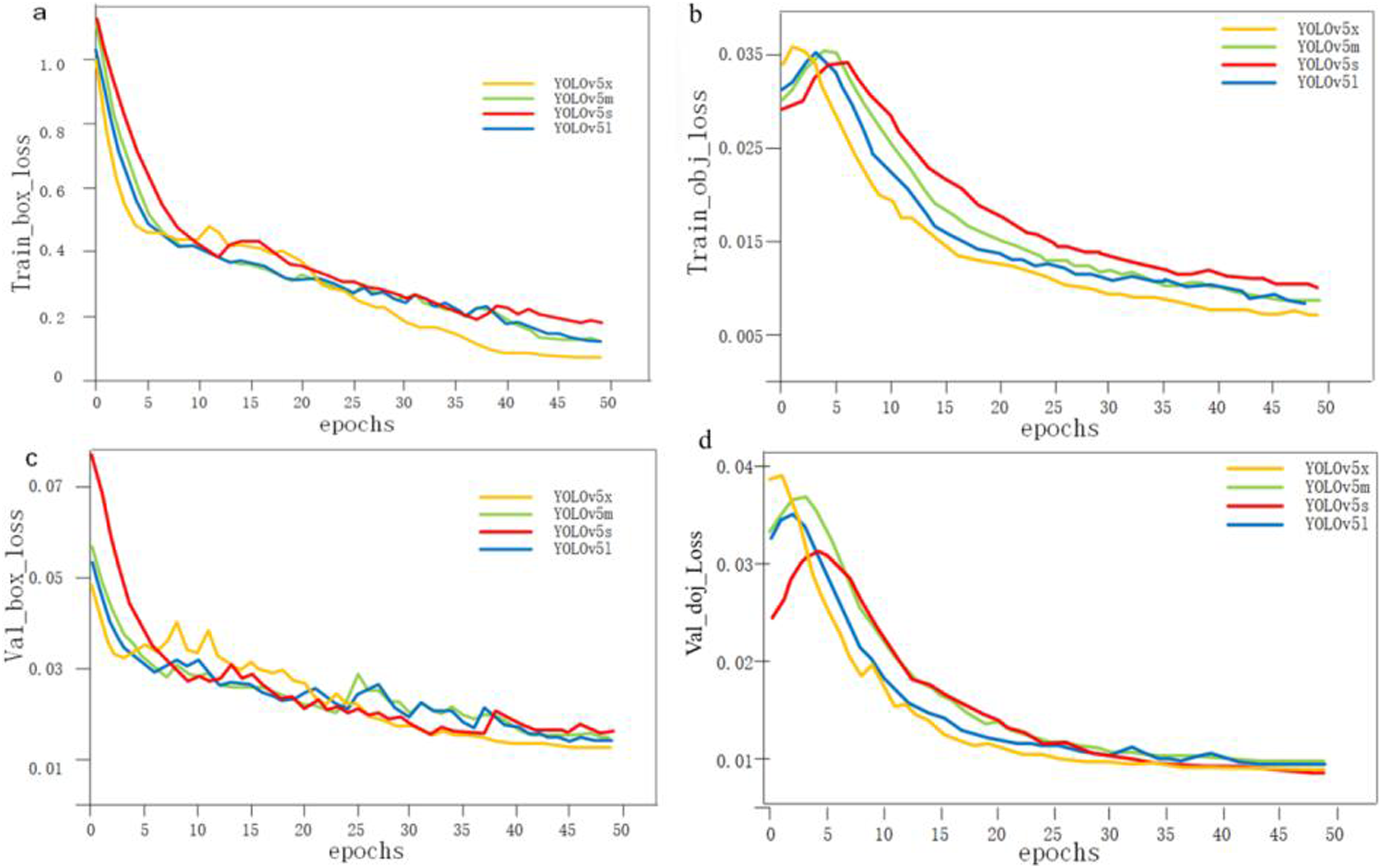

Table 2 shows the values of the loss function for both the training and validation sets of the four models upon the completion of training. The values of both the localization and confidence losses for the YOLOv5x model were smaller than those of the other three models on the training and validation sets. The YOLOv5x model had a lower confidence loss than the YOLOv5s model on the validation set, but the difference between the two was small.

Table 2.

Loss values of four models.

	YOLOv5s	YOLOv5m	YOLOv5l	YOLOv5x
train_box_loss	0.02646	0.01985	0.02221	0.01697
train_obj_loss	9.6789e-3	8.3865e-3	8.3517e-3	7.2613e-3
val_box_loss	0.01757	0.01489	0.01581	0.01284
val_obj_loss	8.8193e-3	9.5452e-3	9.5933e-3	9.228e-3

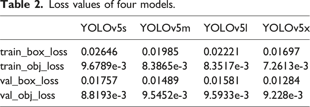
Figure 3(A) and (B) present the precision and recall rates of the four models after training. There was only a minor difference among the four models; all of them achieved over 98% accuracy. The F1 scores and precision–recall (PR) curves of the four models are shown in Figure 3(C) and (D), respectively. The YOLOv5x model performed significantly better than the other models based on the F1 scores. However, the performance differences among the four models were relatively small according to the PR curves.

Figure 3.

Performance metrics of the four models after training: (A) Precision, (B) Recall rates, (C) F1 scores, and (D) Precision-Recall (PR) curves.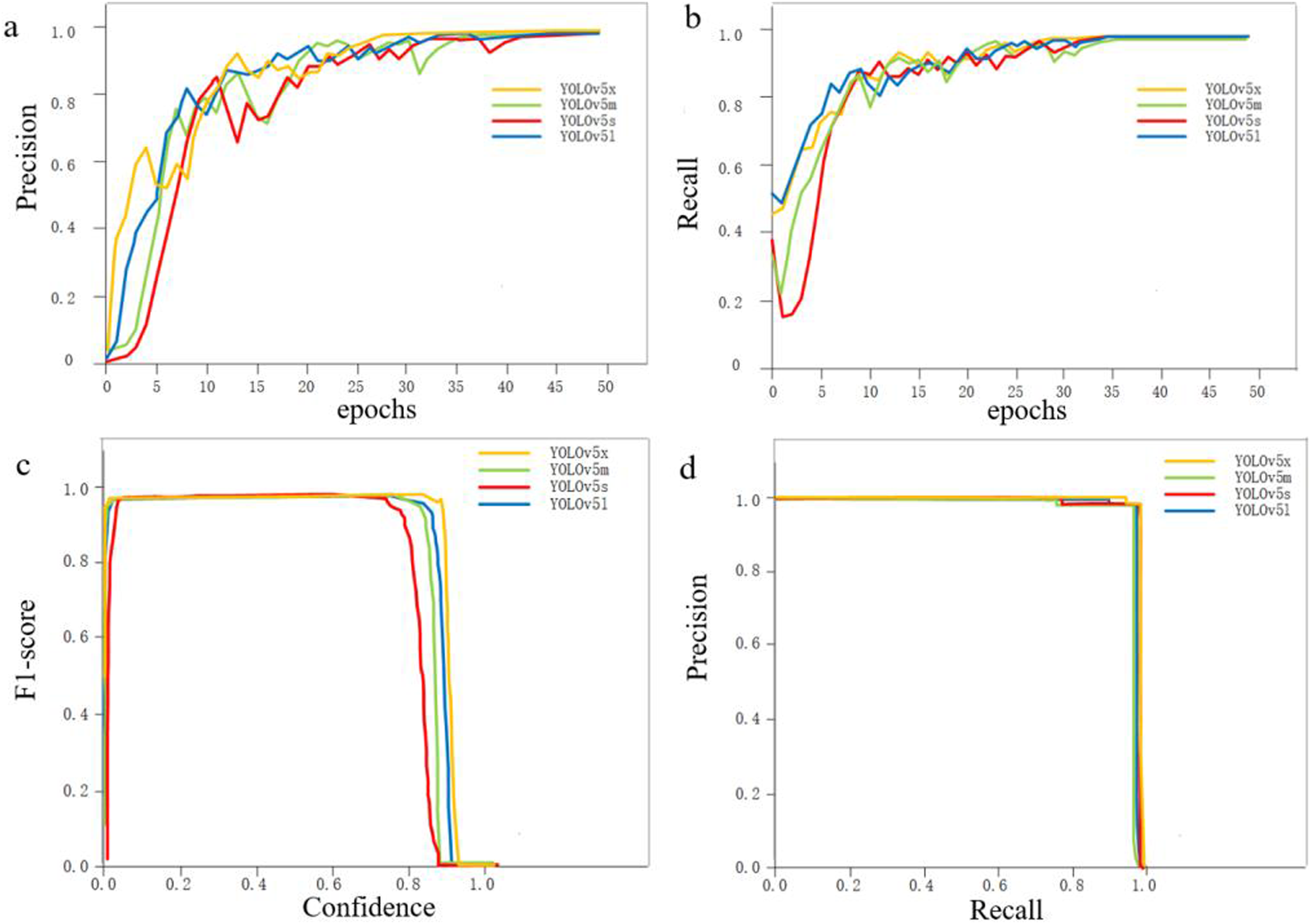

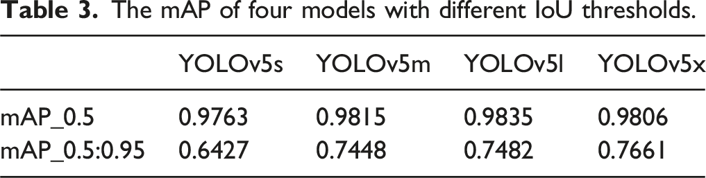
As there was only one category for object detection, mean average precision (mAP) was the same as average precision (AP). At the beginning of training, the threshold was set to 0.5 to obtain the precision and recall rates. These were then used to derive the mAP change graph shown in Figure 4(A). The four models had almost the same average precision. By gradually increasing the IoU threshold size by 0.05 until it reached 0.95 and by calculating the mean mAP at each step, mAP change graphs under this threshold condition were produced (shown in Figure 4(B)). It was evident that the YOLOv5x model had the highest average precision. The detailed mAP values for the two thresholds are listed in Table 3.

Figure 4.

(A) Comparison of mAP at threshold of 0.5; (B) comparison of mAP at thresholds of 0.5 to 0.95.

Table 3.

The mAP of four models with different IoU thresholds.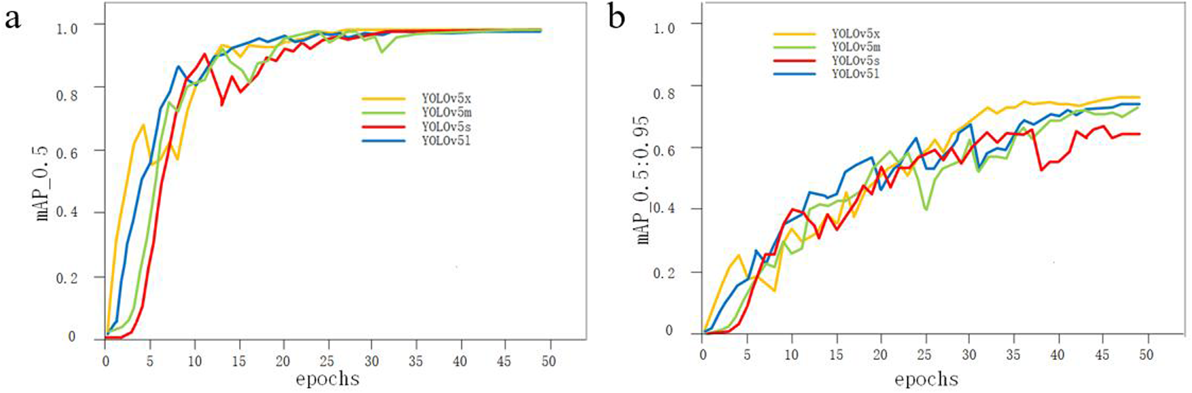

	YOLOv5s	YOLOv5m	YOLOv5l	YOLOv5x
mAP_0.5	0.9763	0.9815	0.9835	0.9806
mAP_0.5:0.95	0.6427	0.7448	0.7482	0.7661

After considering all the indicators, YOLOv5x outperformed the other three models in most aspects, with improved values for both the indicators and the loss functions. A few indicators or loss functions were either on par or slightly lower than the other three models. Based on this analysis, YOLOv5x was the most suitable model for the target detection task of locating back regions when compared with the other three models. The final localization results are shown in Figure 5.

Figure 5.

Localization results of the back region.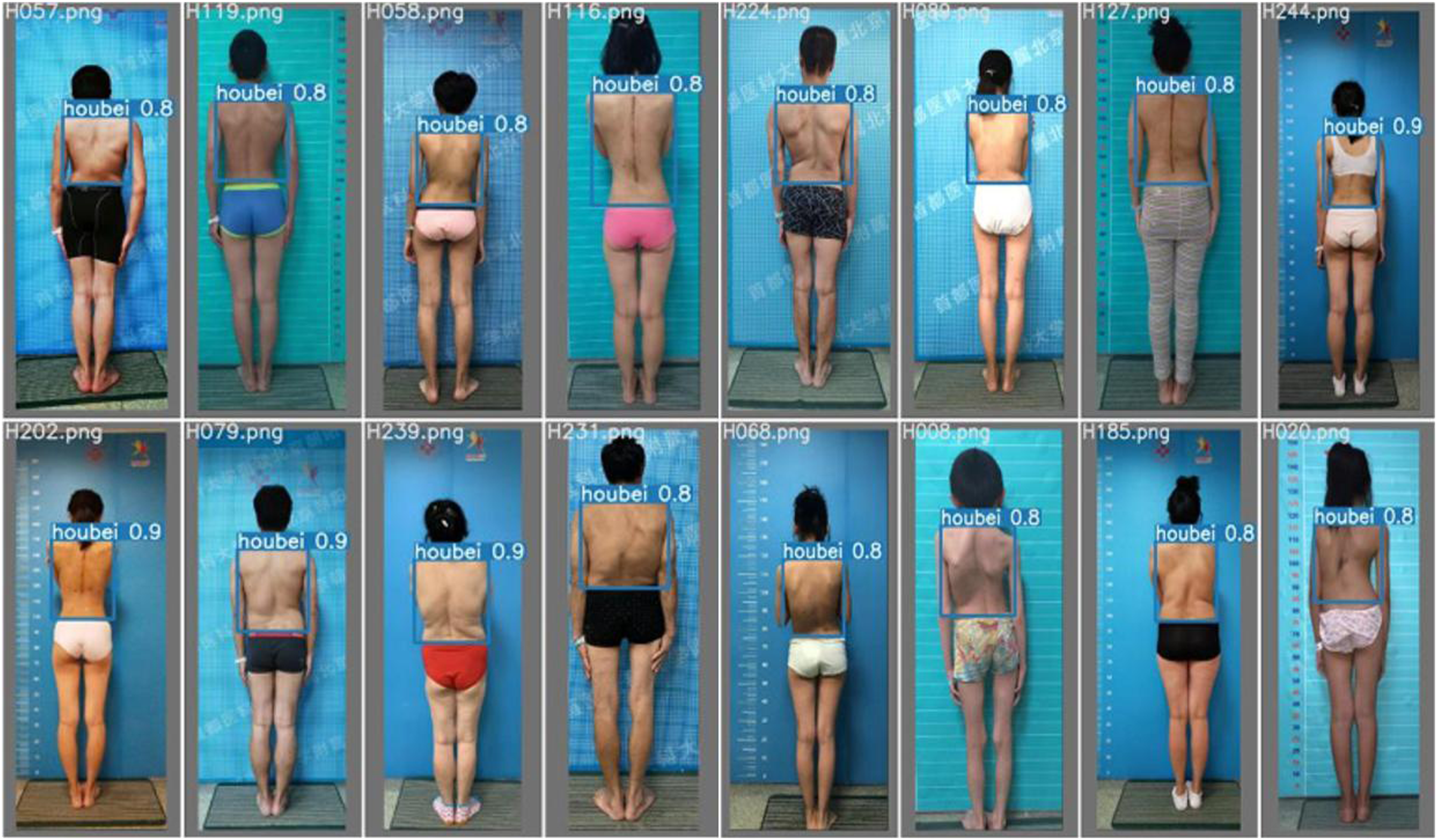

Spine Region Segmentation Results

The loss functions with different learning rates after training are shown in Figure 6. The specific training loss values for different learning rates at the end of training are presented in Table 4.

Figure 6.

Loss curves for models trained under different learning rates. (A) training loss, and (B) validation loss.

Table 4.

Training loss under different learning rates.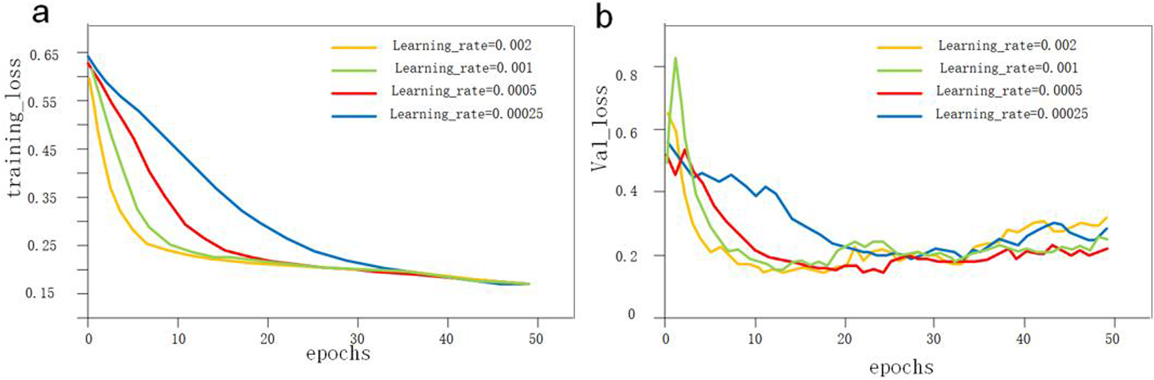

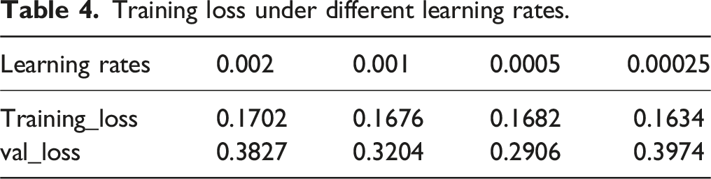
Learning rates	0.002	0.001	0.0005	0.00025
Training_loss	0.1702	0.1676	0.1682	0.1634
val_loss	0.3827	0.3204	0.2906	0.3974

The loss functions for the models under different learning rates all stably converged on the training set, indicating that the models could be successfully trained under these four learning rates. However, on the validation set, the model with the learning rate of 0.0005 achieved the lowest loss value at the end of training, indicating the best training performance. Based on this result, we confirmed that a learning rate of 0.0005 was optimal for the spine segmentation algorithm. The data augmentation and final spine region segmentation results are shown in Figure 7.

Figure 7.

Data augmentation and spinal segmentation results. (A) Original image. (B) image flipping. (C) Gaussian noise injections. (D, E) brightness adjustments. (F, G) Examples of U-Net-Residual Network (ResNet) segmentation effects.injections. (D, E) brightness adjustments. (F, G) Examples of U-Net-Residual Network (ResNet) segmentation effects.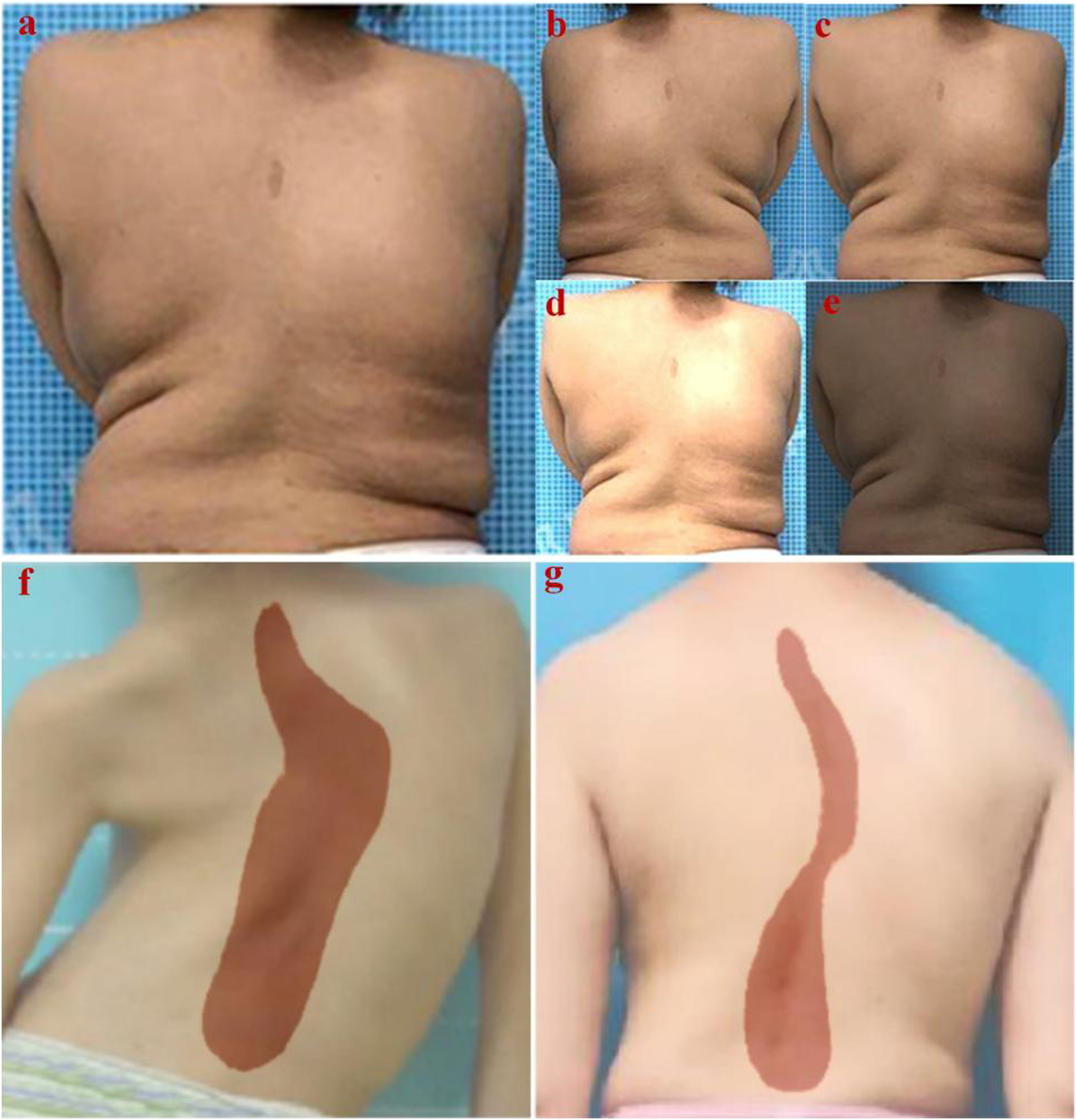

Cobb Angle Measurement Results

Upright images of the backs of 20 groups of scoliosis patients and their corresponding contemporaneous radiograph images were prepared to validate the accuracy of the algorithm developed in this study. By identifying the upper and lower vertebrae of the spine in the radiographic images and measuring their Cobb angle using a protractor, we obtained the control group for this validation. We then used this algorithm to calculate the Cobb angles for 20 sets of upright images of the back. All results were retained as integers by rounding. The final results are shown in Figure 8.

Figure 8.

Comparison of measurement results of different methods.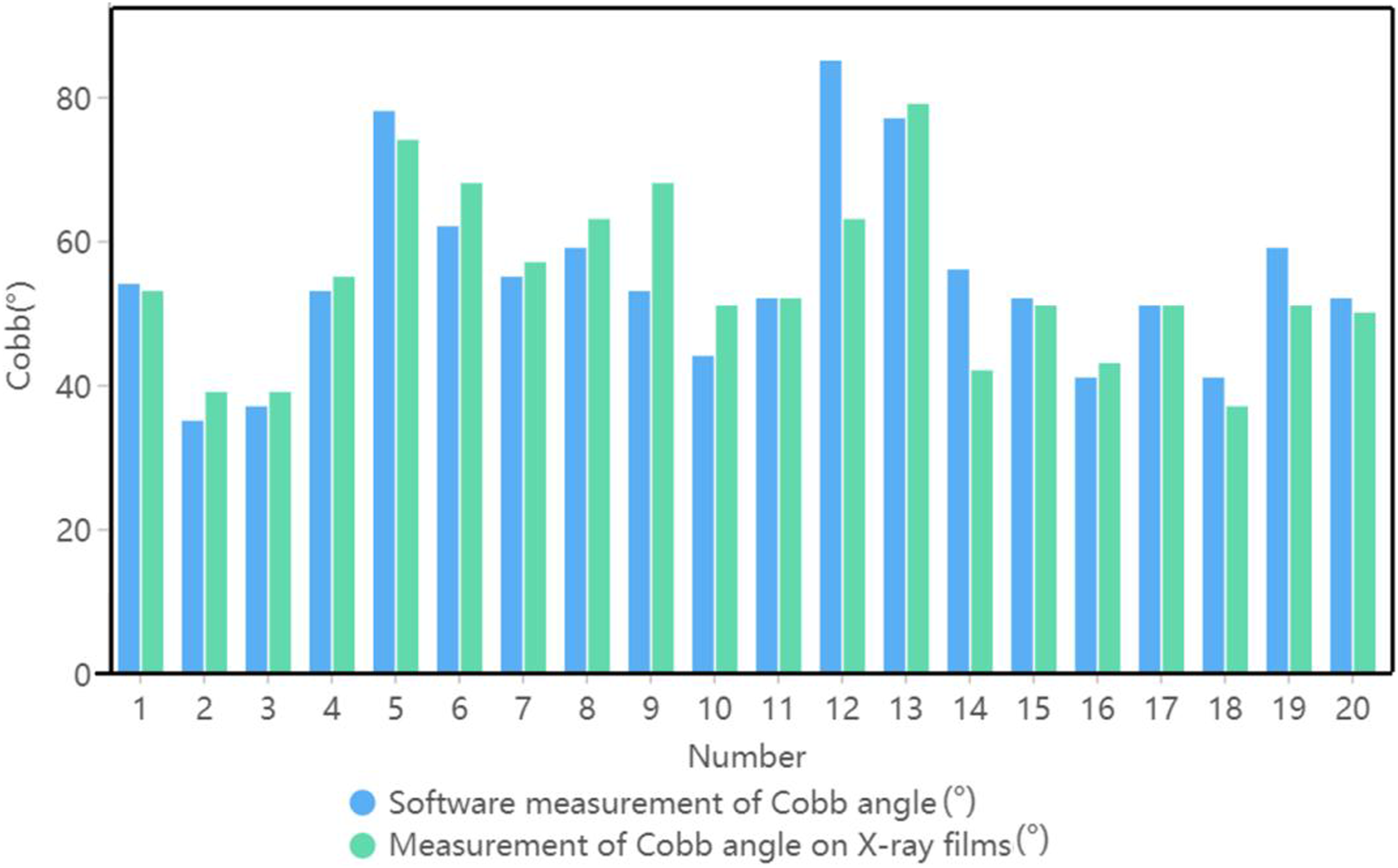

The measurement results showed that 85% of the data had Cobb angle measurement errors within 10° and 80% of the data had Cobb angle measurement errors within 5°. This indicated a good prediction of the Cobb angle, demonstrating the feasibility of this system to screen scoliosis using the Cobb angle measurement from upright images of the back.

Discussion

The results of this study indicated that the proposed system was effective in measuring the Cobb angle and proved the feasibility of screening scoliosis using upright images of the back. This method enabled the initial screening of scoliosis by a prediction of the Cobb angle without requiring a physical examination by a specialized physician, thus reducing the consumption of social and medical resources. Therefore, this system could be used as a mass screening tool for adolescent scoliosis.

Computer-aided diagnosis offers many advantages over traditional scoliosis screening methods. First, instead of relying on X-rays and manual measurements by physicians, intelligent screening requires only bare-leakage photographs of the back to achieve a prediction of the Cobb angle to screen for scoliosis risk. This significantly reduces the cost of screening and the pressure on medical resources. It also dramatically reduces the impact of X-rays on the human body and the probability of cancer caused by X-rays. This significantly reduces the cost of screening and the pressure on medical resources.^23,24 Second, the screening system could automatically predict the Cobb angle without manual work, making it more efficient than traditional screening methods and allowing for the rapid screening of large populations.

Several studies have researched computer-aided scoliosis diagnosis. Ramirez et al.²⁵ Proposed the use of a support vector machine (SVM) model²⁶ combined with clinical data to classify and predict the level of scoliosis in patients, based on their back images. The study reported accuracy values ranging from 69% to 85%. The researchers also found that SVM was more effective for scoliosis classification than other machine learning classifiers such as decision trees. In a 2013 study, Phan et al.²⁷ evaluated adolescent idiopathic scoliosis using a network model of self-organizing maps (SOM)²⁸ and achieved an optimized accuracy of nearly 82%. Similarly, Yang et al.⁷ developed a framework for scoliosis screening based on convolutional neural networks (CNNs),²⁹ targeting upright images of the back. They employed Faster R-CNN CNNs to identify the back part of a person and extract the image with an accuracy of more than 99% whilst avoiding the omission of image features. This method did not require a high image quality, making it practical for screening purposes. Overall, the application of machine learning algorithms and neural networks such as SVM and CNN has shown promising results in accurately classifying and predicting the level of scoliosis. These methods can improve the efficiency and accuracy of scoliosis diagnosis, enabling effective screening even with lower picture qualities.

Analyzing the characteristics of the most accurate and inaccurate patients between software-measured Cobb angles and X-ray film measurements is crucial for understanding the deep learning model’s strengths and weaknesses in diagnosing scoliosis. We have summarized the accuracy data for each image in our dataset, finding that significant measurement deviations often occur in images with excessive brightness or unclear back contours due to obesity.

Currently, neural networks function somewhat as “black box” systems due to the complexity and opacity of their internal workings and decision-making processes. While clinicians manually extract spinal features with clear justifications, neural networks approximate the training set with less transparent methods. Despite these challenges, we can enhance the model’s generalization by increasing the training set’s size and diversity and incorporating more network layers. In summary, while deep learning models hold promise for large-scale scoliosis screenings without X-rays, future research should focus on clarifying neural network feature selection and optimizing training to improve diagnostic accuracy.

This study had several limitations. First, although Cobb angle measurement is the gold standard for diagnosing scoliosis, incorporating additional indicators during early screening can provide a more comprehensive assessment. Specifically, parameters such as shoulder height discrepancy, scapular symmetry, and coracoid height are vital. Shoulder height discrepancy can be observed through the alignment of the shoulders, while scapular symmetry involves comparing the positions and rotations of the scapulae relative to each other. Coracoid height, though typically measured with more interior landmarks, can be inferred from changes in the shoulder contour. Incorporating these visual indicators can help in identifying scoliosis early.³⁰ Second, during large-scale scoliosis screening, image acquisition involves the privacy of the test subjects. Therefore, screening and diagnosing upright image data of the back with tight-fitting clothing should be investigated. Due to limited samples, the accuracy of this method needs further improvement. Finally, Our current dataset is dependent on specialized clinicians who manually annotate feature points on back x-rays. The precise location of these feature points directly impacts the localization accuracy of our system. However, this manual process is time-consuming and labor-intensive, thereby constraining the dataset’s size. To expedite dataset creation, we propose enhancing the process by reducing the number of feature points and increasing the number of collaborating clinicians, among other strategies. In the future, we aim to scale the dataset more efficiently, ultimately improving the system’s overall performance.

Conclusions

In this study, we proposed a new method that incorporates deep learning for the automated localization of back ROIs, spinal region segmentation, and Cobb angle measurements. While the initial results indicate that the proposed method achieves high efficiency, it is not yet as accurate as traditional human visual recognition. However, the method is automated, concise, and convenient, showing great potential for improving over time with further development. Future work involves applying our method to scoliosis screening in primary and secondary schools and collecting additional databases to enhance model performance.

Footnotes

Acknowledgments

We would like to thank all the supporter and participants in our research.

Authors’ Contributions

Conceptualization, B.P. and X.W.; methodology, L.Z.; software, L.Z., D.L., and S.Z.; investigation, B.P.; resources, B.P.; data curation, X.W., L.Z., and S.Z.; writing—original draft preparation, B.P. and L.Z.; writing—review and editing, B.P., L.Z. and X.W.; visualization, X.H.; supervision, Y.X.; project administration, X.W.; funding acquisition, B.P.

Declaration of Conflicting Interests

The author(s) declared no potential conflicts of interest with respect to the research, authorship, and/or publication of this article.

Funding

The author(s) disclosed receipt of the following financial support for the research, authorship, and/or publication of this article: This work was supported by the Guangdong Basic and Applied Basic Research Foundation (2023A1515110378) and Beijing Natural Science Foundation (L232004)

Ethical Statement

ORCID iD

Le Zhang

Data Availability Statement

The data that support the findings of this study are available from the corresponding author upon reasonable request.*

References

Cheng

Castelein

Chu

, et al. Adolescent idiopathic scoliosis. Nat Rev Dis Prim. 2015;1:15030.

Moramarco

Borysov

, et al. Schroth’s Textbook of Scoliosis and Other Spinal Deformities. Cambridge: Cambridge Scholars Publishing; 2020.

Rothstock

Weiss

Krueger

Kleban

Paul

. Innovative decision support for scoliosis brace therapy based on statistical modelling of markerless 3D trunk surface data. Comput Methods Biomech Biomed Eng. 2020;23(13):923-933.

Villamor

Andras

Yang

Skaggs

. Psychological effects of the SRS-22 on girls with adolescent idiopathic scoliosis. Spine Deform. 2018;6(6):699-703.

Gurovich

Hanani

Bar

, et al. Identifying facial phenotypes of genetic disorders using deep learning. Nat Med. 2019;25(1):60-64.

Poplin

Varadarajan

Blumer

, et al. Prediction of cardiovascular risk factors from retinal fundus photographs via deep learning. Nat Biomed Eng. 2018;2(3):158-164.

Yang

Zhang

Fan

, et al. Development and validation of deep learning algorithms for scoliosis screening using back images. Commun Biol. 2019;2:390.

Ronckers

Land

Miller

Stovall

Lonstein

Doody

. Cancer mortality among women frequently exposed to radiographic examinations for spinal disorders. Radiat Res. 2010;174(1):83-90.

Ronneberger

Fischer

Brox

. U-Net: convolutional networks for biomedical image segmentation. MICCAI. 2015;9351:234-241.

10.

Chi

Wang

Hao

Xia

. Residual network and embedding usage: new tricks of node classification with graph convolutional networks. J Phys Conf Ser. 2022;2171:012011.

11.

Sun

Qin

Gao

Chai

Chen

. Attention-enhanced multi-scale residual network for single image super-resolution. Signal Image Video Process. 2022;16(5):1417-1424.

12.

Qiu

Cheng

Wang

. Dual U-Net residual networks for cardiac magnetic resonance images super-resolution. Comput Methods Progr Biomed. 2022;218:106707.

13.

Maharjan

Alsadoon

Prasad

PWC

Al-Dalain

Alsadoon

. A novel enhanced softmax loss function for brain tumour detection using deep learning. J Neurosci Methods. 2020;330:108520.

14.

Tai

Chen

Niu

Chen

Lai

. Application of two-parameter scoliometer values for predicting scoliotic cobb angle. Biomed Eng Online. 2017;16(1):136.

15.

Chlap

Min

Vandenberg

Dowling

Holloway

Haworth

. A review of medical image data augmentation techniques for deep learning applications. J Med Imaging Radiat Oncol. 2021;65(5):545-563.

16.

Erickson

Korfiatis

Akkus

Kline

. Machine learning for medical imaging. Radiographics. 2017;37(2):505-515.

17.

Lim

Loo

Tran

, et al. DOPING: generative data augmentation for unsupervised anomaly detection with GAN. 2018 IEEE International Conference on Data Mining (ICDM), Singapore, 17-20 November 2018:1122-1127.

18.

Xie

Dai

Hovy

, et al. Unsupervised data augmentation for consistency training. NIPS. 2019;20:6256-6268.

19.

Zheng

Jin

Dong

. Rail detection based on LSD and the least square curve fitting. Int J Autom Comput. 2021;18(01):85-95.

20.

Layade

Adebo

Olurin

, et al. Separation of regional-residual anomaly using least square polynomial fitting method. JNAMP. 2015;30(0):169-180.

21.

Simpson

. Least squares polynomial fitting to gravitational data and density plotting by digital computers. Geophysics. 1954;19(2):255-269.

22.

Schork

Gondzio

. Rank revealing Gaussian elimination by the maximum volume concept. Linear Algebra Appl. 2020;592(C):1-19.

23.

Stewart

. Python for Scientists. 2nd ed. Cambridge: Cambridge University Press; 2017.

24.

Ronckers

Doody

Lonstein

Stovall

Land

. Multiple diagnostic X-rays for spine deformities and risk of breast cancer. Cancer Epidemiol Biomarkers Prev. 2008;17(3):605-613.

25.

Ramirez

Durdle

Raso

Hill

. A support vector machines classifier to assess the severity of idiopathic scoliosis from surface topography. IEEE Trans Inf Technol Biomed. 2006;10(1):84-91.

26.

Nie

Zhu

. Decision tree SVM: an extension of linear SVM for non-linear classification. Neurocomputing. 2020;401:153-159.

27.

Phan

Mezghani

Wai

de Guise

Labelle

. Artificial neural networks assessing adolescent idiopathic scoliosis: comparison with lenke classification. Spine J. 2013;13(11):1527.

28.

Kovačević

Pasquato

Marelli

De Luca

Salvaterra

Belfiore

. Exploring X-ray variability with unsupervised machine learning. Age (Chester). 2022;659:A66.

29.

Lecun

Bengio

, eds. Convolutional networks for images, speech, and time-series. The Handbook of Brain Theory and Neural Networks. Cambridge: MIT Press; 1995:255-258.

30.

Fong

Cheung

Wong

, et al. A population-based cohort study of 394,401 children followed for 10 years exhibits sustained effectiveness of scoliosis screening. Spine J. 2015;15(5):825-833.

A New Method for Scoliosis Screening Incorporating Deep Learning With Back Images

Abstract

Study Design

Objectives

Methods

Results

Conclusions

Keywords

Introduction

Materials and Methods

Image Localization

Data Acquisition

Annotation Process

Network Training

Evaluation Metrics for Network Performance

Automatic Spinal Segmentation Algorithm Construction

Network Architecture and Loss Function Design

Data Preprocessing

Network Training and Performance Analysis

Polynomial Fitting of Spinal Curves Based on Least Squares Method

Cobb Angle Automated Measurement

Results

Localization Results of the Back Region

Spine Region Segmentation Results

Cobb Angle Measurement Results

Discussion

Conclusions

Footnotes

Acknowledgments

Authors’ Contributions

Declaration of Conflicting Interests

Funding

Ethical Statement

ORCID iD

Data Availability Statement

References