Sage Journals: Discover world-class research

Abstract

Study design

Retrospective data analysis.

Objectives

This study aims to develop a deep learning model for the automatic calculation of some important spine parameters from lateral cervical radiographs.

Methods

We collected two datasets from two different institutions. The first dataset of 1498 images was used to train and optimize the model to find the best hyperparameters while the second dataset of 79 images was used as an external validation set to evaluate the robustness and generalizability of our model. The performance of the model was assessed by calculating the median absolute errors between the model prediction and the ground truth for the following parameters: T1 slope, C7 slope, C2-C7 angle, C2-C6 angle, Sagittal Vertical Axis (SVA), C0-C2, Redlund-Johnell distance (RJD), the cranial tilting (CT) and the craniocervical angle (CCA).

Results

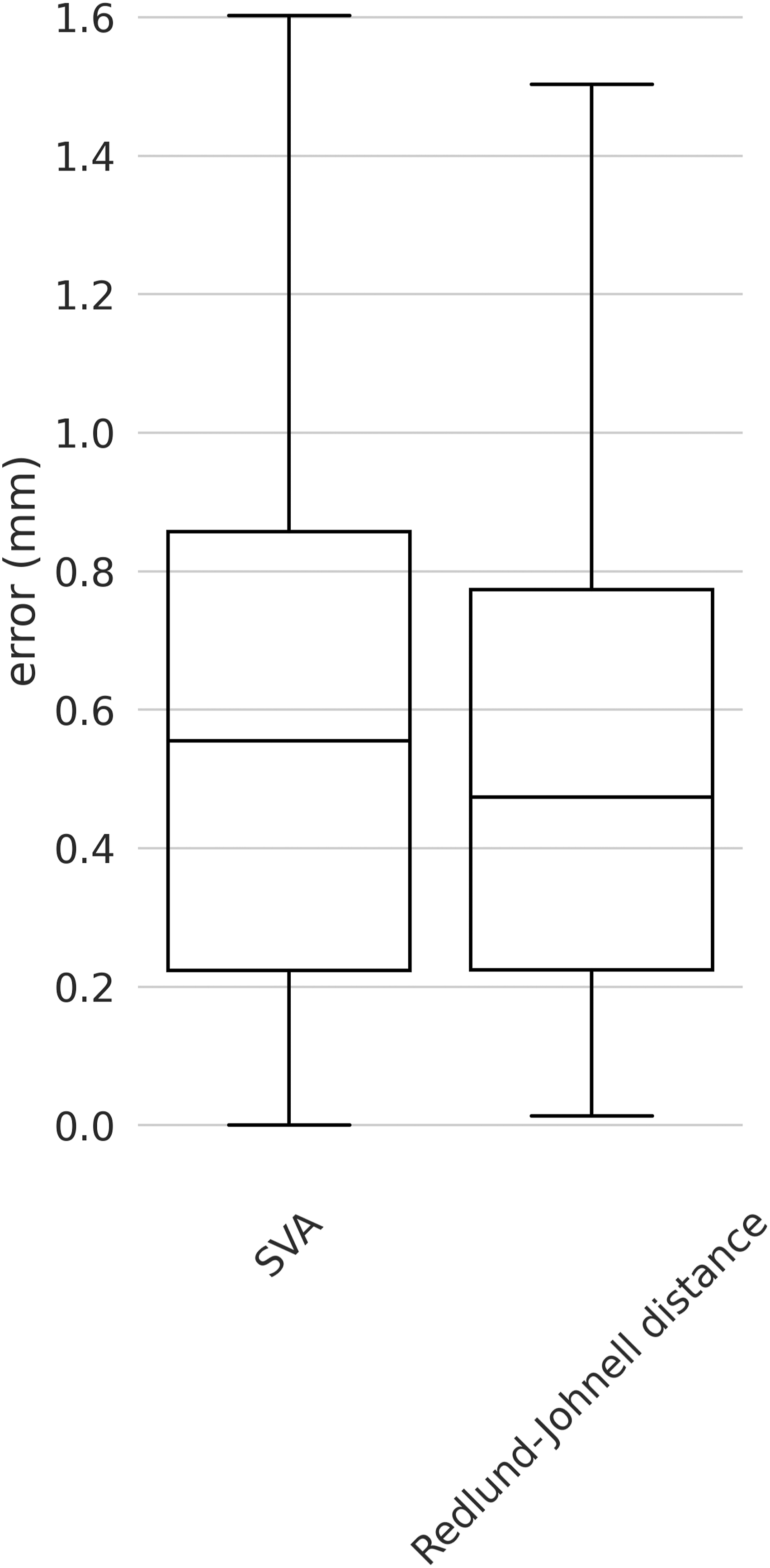
Regarding the angles, we found median errors of 1.66° (SD 2.46°), 1.56° (1.95°), 2.46° (SD 2.55), 1.85° (SD 3.93°), 1.25° (SD 1.83°), .29° (SD .31°) and .67° (SD .77°) for T1 slope, C7 slope, C2-C7, C2-C6, C0-C2, CT, and CCA respectively. As concerns the distances, we found median errors of .55 mm (SD .47 mm) and .47 mm (.62 mm) for SVA and RJD respectively.

Conclusions

In this work, we developed a model that was able to accurately predict cervical spine parameters from lateral cervical radiographs. In particular, the performances on the external validation set demonstrate the robustness and the high degree of generalizability of our model on images acquired in a different institution.

Keywords

radiology deep learning landmarks localization automatic parameters calculation cervival radiographs cervical spine

Introduction

The complexity of the cervical spine alignment originates from the interrelationship between the head, the thoracolumbar alignment as a flexible base, and the lower extremities. The investigation of the cervical spine alignment is becoming increasingly valuable as the relationship between proper sagittal alignment and better clinical outcomes is better understood.^1-4 Multiple cervical spine studies have looked at relationships between cervical alignment and the occurrence of adjacent segmental disease namely complications of spinal fusion,⁵ and studies over the last several years have revealed the relationship with health-related quality of life (HRQOL).⁶ Although the cervical spine determines only a local part of the global spinal alignment, its clinical importance is high.² One example of this is given by postoperative dyspnea and dysphagia, which are strongly influenced by the angle of the occipito-cervical junction.⁷

Currently, surgeons and radiologists primarily perform cervical spine alignment measurements manually. While many improvements in the manual cervical spine measurements have been reported owing to the use of computer-assisted tools, the manual evaluation of medical images can take several minutes and is prone to human error.^8-10 Therefore, there is still room for innovation in cervical spine image analysis; machine learning has the potential to solve some of the issues related to manual evaluation.

Automated image analysis in the field of spine surgery is an active area of research. Initially, the measurement of Cobb angle was the main focus of interest, but advances in machine learning and computer vision in recent decades have led to an increasing number of researchers interested in the automated measurement of spinal parameters such as lordosis angles, T4-T12 kyphosis, sacral slope and pelvic incidence.^11-13 Schwartz et al reported that an automated algorithm measures spinal and pelvic parameters in lateral radiographs of the lumbar spine with accuracy comparable to that of a surgeon.¹⁴ Several reports also found the intraclass correlation coefficient (ICC) of the algorithm compared to human raters to be good to excellent.^15,16 In previous work, the authors used a two-step deep learning model to calculate lumbar spine parameters and reported absolute median errors of 2.43° for L1-S1 lordosis and 1.98° for sacral slope.¹⁷ These results were good with respect to the intra-rater variability of such parameters ranging from .8 to 5 degrees¹⁸ When it comes to the cervical spine, there have been only a few reports about automated image analysis,^19-22 which did not provide a comprehensive measurement of cervical parameters, and are therefore difficult to apply in clinical use.

The purpose of this study was to develop a new automated image analysis algorithm for the comprehensive measurement of cervical spine alignment parameters in lateral radiographs and to evaluate its accuracy in comparison to human examiners on an external validation set. In particular, starting from the model,¹⁷ we developed and validated a deep learning model to automatically calculate 29 cervical spine landmarks, with the overarching goal to compute a comprehensive set of cervical spine alignment parameters from these landmarks.

Materials and Methods

Datasets

Two distinct datasets were used in the present study. The first dataset consisted of 3466 fully anonymized lateral uncalibrated x-ray images of the cervical spine acquired from the database of BLINDED FOR REVIEW. All the images were from an individual patient. Ethical approval was obtained from the relevant institutional review board (BLINDED FOR REVIEW), and informed consent requirement was exempted. To obtain a sufficiently large number of images for the subsequent analyses, with/without pathology, and instrumented images as well as images of young and elderly people were included. We used a wide variety of images since our goal was to build a robust model that could deal with many different cases. The following 29 landmarks were manually annotated in the (x, y) coordinates by an experienced orthopedic surgeon: four corners of vertebral bodies corresponding to spine level from C2 to C7, two corners of the upper endplate of T1, two points to draw the McGregor line at the posterior margin of the hard palate and the lowermost edge of occiput, and the tip of C2 dens process. The second dataset consisted of 197 images of individual patients taken from an existing anonymized dataset from the BLINDED FOR REVIEW. For this dataset, the same 29 points described above were annotated by the same surgeon that annotated the first dataset and by three other annotators.

For both datasets, images fulfilling at least one of the following criteria were excluded: unidentified McGregor line; unidentified T1 upper endplate; unidentified landmarks due to fused vertebrae; unphysiological position of the landmarks due to vertebral fracture. After applying the exclusion criteria, the remaining images of the first dataset were split into a train set (80%) and a test set (20%) which were used to train the model and to optimize its parameters respectively. All images belonging to the second dataset were used exclusively for the external validation of the model.

Deep Learning Model

Landmark localization in computer vision has undergone significant developments over the years. Initially, standard algorithms relied on feature extraction and matching techniques to locate landmarks in images.²³ However, these methods had limitations when dealing with complex and heterogeneous objects such as the spine. The emergence of deep learning revolutionized landmark localization. Convolutional Neural Network (CNN)-based models proved highly effective by learning the mapping between images and landmark positions through training on annotated datasets.²⁴ The idea is to process the image through different layers of the neural network to automatically extract useful features and patterns from the images. Deep learning approaches provided superior accuracy compared to traditional algorithms. Further progress led to heatmap-based approaches in deep learning. Instead of predicting landmark coordinates directly, these methods generated heatmaps, highlighting the presence and location of landmarks within the image.²⁵ Heatmap-based approaches proved more robust to occlusions and lighting variations, resulting in even more precise and reliable landmark localization.

Today, the field of landmark localization continues to advance, leveraging the power of deep learning techniques and heatmap-based strategies to achieve remarkable results in various computer vision applications.²⁶ For our work, we used a heatmap-based approach. We developed the deep learning model starting from the two-step model described in.¹⁷ Instead of using two separate steps, namely two different training steps aimed at performing a coarse and a fine localization separately, we developed an end-to-end model that first performs a coarse localization to extract the bounding boxes and then refines the localization of the landmarks within the bounding boxes (Figure 1). Finally, the coordinates of the landmarks computed in the bounding boxes space needed to be rescaled back to the space of the original image.

Figure 1.

Model architecture. The entire images are first processed by the hourglass model to produce a first prediction of the (x, y) coordinates. The coordinates from the upper endplate of T1 to the lower endplate of C2 are used to extract the bounding boxes from the images. Then, 6 models are used to predict more precisely the locations of the four corners that surround the intervertebral discs from C7-T1 to C2-C3. The 24 corners are then projected back to the original images and added to the 5 points from the global model to predict the set of 29 points. The 24 points locally predicted are displayed in red, while the 5 points globally predicted are displayed in yellow.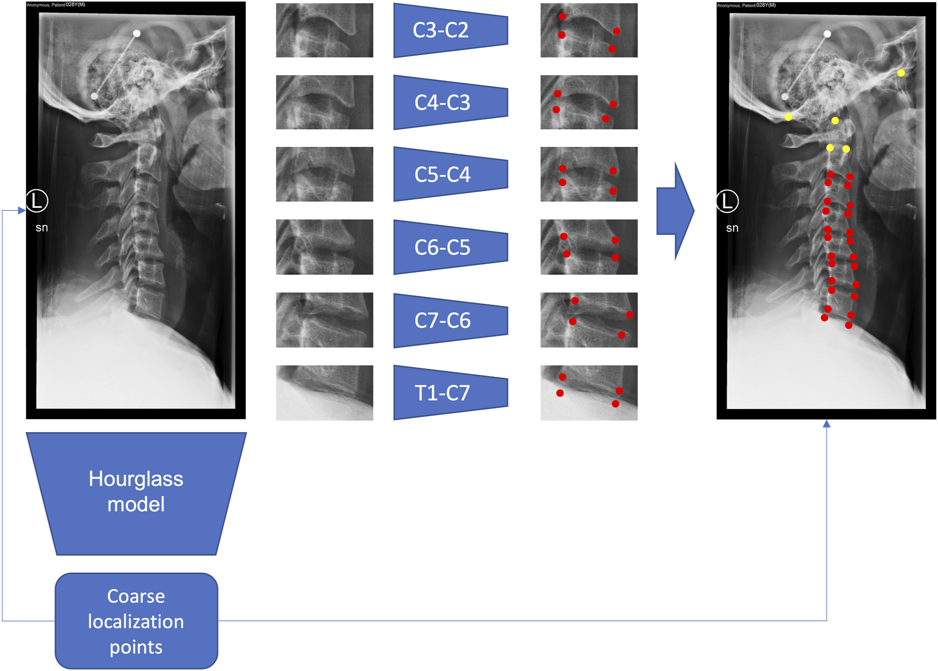

This algorithm was applied only to the landmarks from the upper endplate of T1 to the lower endplate of C2, whereas the remaining points (upper corners of C2, posterior margin of the hard palate, lowermost edge of occiput, dens tip) were localized directly in the original image without using bounding boxes. Hence, we used six bounding boxes around the intervertebral discs from C7-T1 to C2-C3 to predict 24 out of 29 landmarks (Figure 1). The model for the full image was an hourglass network²⁵ with two stacked hourglass modules while each one of the six models used for the refinement is an hourglass network with only one hourglass module, inspired by the work of Chandran et al on face points detection.²⁷ For all the models, on top of the last convolutional layer feature map we used the DSNT layer²⁸ that was already used in¹⁷ to perform the coordinates regression using a spatial to numerical transformation from the spatial heatmaps. To make the network fully differentiable we used the roialign function from PyTorch²⁹ to extract the bounding boxes using the coarse localization coordinates.

All the images were scaled to 1024 × 1024 resolution using bicubic interpolation and were normalized to have zero mean and unit variance. The extracted bounding boxes for refinement were rescaled to 128 × 128 resolution. We applied augmentation techniques such as rotation (−5 to 5 degrees), scaling (.8 to 1.2 of original dimension), small translation, and gaussian noise to the input images to make the model more robust. Regarding training details, for the coarse localization model we used the Euclidean distance between the predicted and the ground truth points as the loss plus a regularization term that computes the divergence between the heatmaps generated from the ground truth coordinates and the heatmaps predicted by the model (equation (1)),²⁸ since the heatmaps can be seen as probability distributions of the points' locations. The loss is calculated as

L 1 = {‖ p - g t ‖}^{2} + D ({h m}_{g t}, {h m}_{p})

(1)

where p represents the predicted coordinates, gt the ground truth coordinates,

{‖ . ‖}^{2}

is the euclidean distance, and D is the divergence between the ground truth heatmaps (

{h m}_{g t}

) and the predicted heatmaps (

{h m}_{p}

For the six refinement models we only used the Euclidean loss (equation (2)) since the ground truth coordinates in the bounding box space were not known in advance, making the computation of the ground truth heatmaps impossible. The corresponding equation is

L 2 = {‖ p - g t ‖}^{2}

(2)

where, as before, p represents the predicted coordinates and gt the ground truth coordinates.

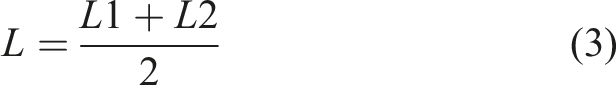
The total loss was then computed by averaging the global model loss and the refinement model loss (equation (3)) as

L = \frac{L 1 + L 2}{2}

(3)

where L1 and L2 are the losses for the first coarse localization model and the refinement models respectively.

We trained the model for 100 epochs using 20 “warmup” epochs optimizing only the coarse localization to have a good starting point for the refinement. We used a batch size of 4 and a starting learning rate of .001 which was reduced by a factor of .1 if there was no improvement in the loss after at least 10 epochs.

We implemented the model in PyTorch and the image augmentation in Albumentations library (https://albumentations.ai/). The model ran on a Linux workstation equipped with an NVIDIA GeForce RTX 3080 with 10 GB of dedicated memory.

Evaluation

The cervical spine parameters that were calculated based on the coordinates of the landmarks were: C2-C7 and C2-C6 lordosis (“C2-C7” and “C2-C6” in the figures and text below), C0-C2 angle (“C0-C2”), C7 slope, T1 slope, C2-7 sagittal vertical axis (“SVA”), the Redlund-Johnell distance (RJD), the cranial tilting (CT) and the craniocervical angle (CCA). The lordosis angle is defined as the Cobb angle formed by two straight lines drawn parallel to the C2 lower endplate and the C6 or C7 lower endplate, and the C0-C2 is measured between the McGregor line and the straight line drawn parallel to the C2 lower endplate. C7 slope and T1 slope are the angles at which the horizontal line intersects the line drawn at the superior endplate of C7 and T1, respectively. SVA is the distance between the plumb line dropped from the centroid of C2 and the posterior superior corner of C7. The RJD was firstly developed for evaluating the vertical dislocation in rheumatoid arthritis patients and is defined as the distance from the lower endplate of C2 to McGregor’s line.³⁰ The CT, designed to evaluate craniocervical parameters, was defined as the angle formed between the line from the center of the T1 upper endplate to the tip of the dens and the sagittal vertical line from the T1 superior endplate, as in the original paper.³¹ The CCA was defined as the angle between the line from the center of C7 to the posterior corner of the hard palate and the McGregor line, as previously reported.³² For all these parameters, the predictions of the model were qualitatively and quantitatively compared to the human annotations.

Moreover, on the external validation set, we performed a more thorough analysis by also investigating the influence of surgical implants and the severity of degenerative changes (recorded for each level) on the performance of the algorithm. For the evaluation of degeneration, we used the Kellgren-Lawrence classification (KL) which indicates: grade zero as definite absence of radiographic changes of osteoarthritis; grade 1 as doubtful joint space narrowing and possible osteophytic lipping; grade 2 as definite osteophytes and possible joint space narrowing; grade 3 as moderate multiple osteophytes, definite narrowing of joint space and some sclerosis and possible deformity of bone ends; grade 4 as large osteophytes, marked narrowing of joint space, severe sclerosis and definite deformity of bone ends.^8,33 The KL grade was binarized on a scale of 0-2 and 3-4, with the grade rated by the majority of the evaluators being adopted.

First, we performed a qualitative evaluation by plotting the points predicted by the model with respect to the distribution of the four annotations to observe if the predictions were consistent with the annotations. Then we represented, for each parameter, the prediction of the model vs the annotators’ range to investigate if the parameters predicted by the model were inside the range of the four annotations. We also used the annotators’ range plus a tolerance of ±2.5° for the angles and ±1 mm for the distances. The range of variability was also used for a more quantitative evaluation to calculate, for each parameter, how many predictions were inside the annotators’ range. In this case, we stratified the angles and distances values in different ranges to investigate if the model makes more mistakes for higher values of the angles and distances. The ranges were 0-10°, 10-20°, 20-30°, 30-40°, >40° for the angles and 0-10 mm, 10-20 mm, 20-30 mm, 30-40 mm, 40-50 mm, >50 mm for the distances.

The performances were evaluated by computing the errors as the absolute differences between the ground truth and the predicted parameters and then by computing the median of the errors. For the external validation set, we used the mean of the four annotations as the ground truth. Moreover, for the external validation set, we computed the intra-class correlation coefficient (ICC) for the parameters both among the annotators to evaluate their agreement and between the mean of the four annotations and the deep learning model. ICC values less than .5 were indicative of poor reliability, between .5 and .75 moderate reliability, between .75 and .9 good reliability, while values greater than .90 indicated excellent reliability.³⁴ Finally, to evaluate if the instrumentation and the degree of the generation affected model performances in terms of landmarks localization, we computed the percentage of points that are predicted inside a certain distance (in millimeters) from the ground truth for the set of images with and without instrumentation, and those with and without degeneration. All the analyses and the plots were generated using Python 3.9 with the seaborn,¹ numpy² and pingouin³ libraries.

Results

After applying the exclusion criteria, 1498 images were kept from the first dataset and were randomly split into 1198 and 300 images for training and testing the model, respectively. Of the 197 images of the external validation set, 79 images (40.1%) could be annotated by all four examiners, one surgeon, one neurosurgeon, and two engineers, while the remaining images were excluded: 69 (35.0%), unidentified McGregor line; 44 (22.3%), unidentified T1 upper endplate; 20 (10.2%), unidentified landmarks due to fused vertebrae; 3 (1.5%), significant change in landmarks due to vertebral fracture. Anterior cervical implants, cages, metal plates, or artificial disc prostheses were included at 48 (10.1%) intervertebral disc levels of 29 (36.7%) annotated testing images, whereas posterior cervical implants were included in 3 images (3.8%). The levels without implants were graded by the KL classification, with 102 (23.9%) levels classified as grade 3-4.

External Validation

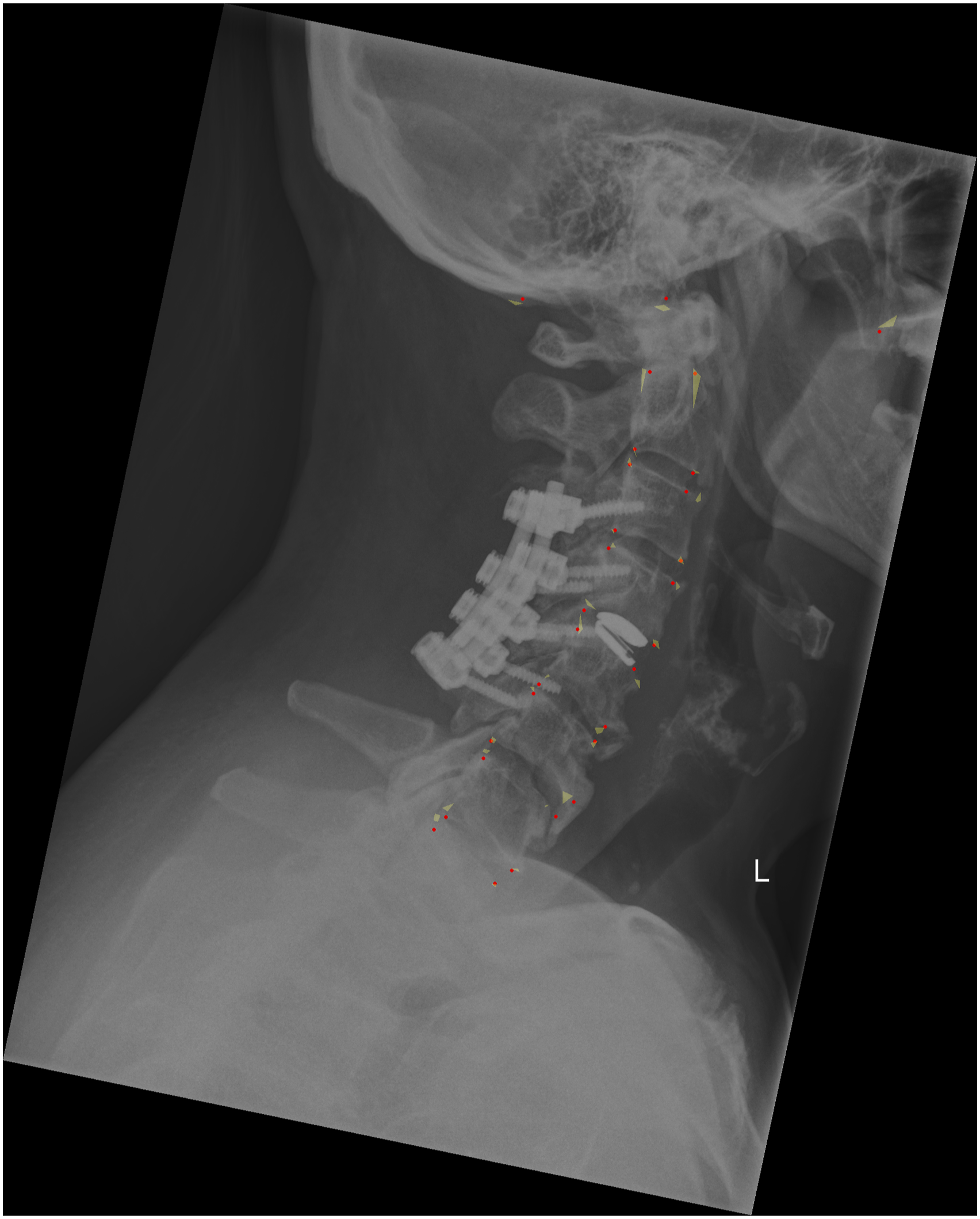
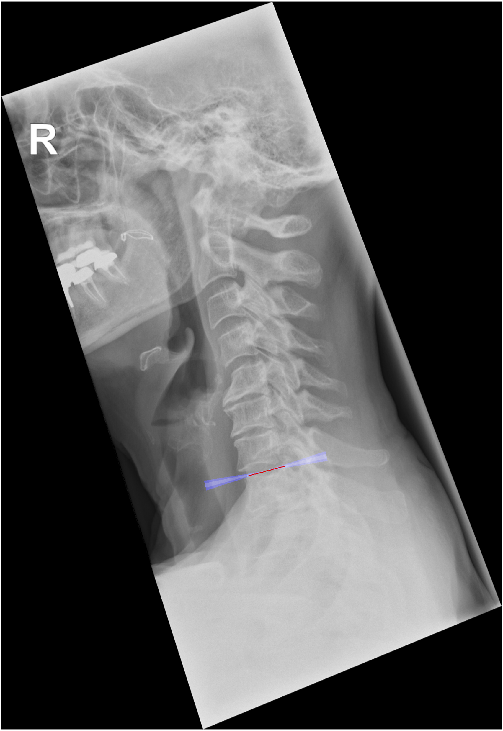
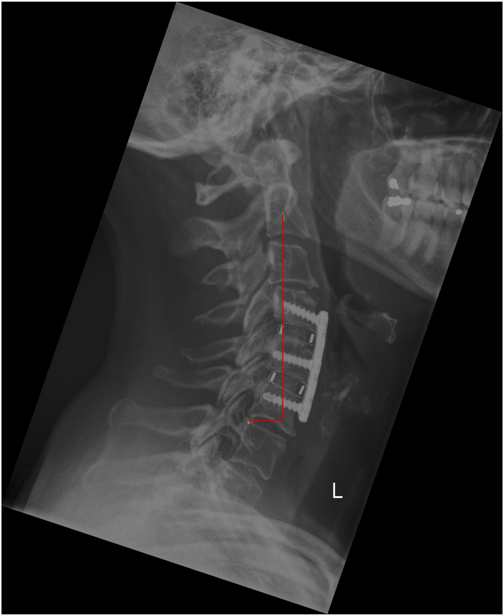
For the external validation set, we first calculated the ICC to observe the agreement among the four annotators, which resulted very high for all the cervical spine parameters with values of .88 (T1 slope), .95 (C7 slope), .94 (C2-C7), .94 (C2-C6), .99 (SVA), .92 (C0-C2), .99 (CT), .97 (RJD), and .96 (CCA) (Figure 2). The qualitative evaluation showed very close agreement between the predictions of the model and the annotations (Figure 3); while the variability of the annotations was very small, the model was able to precisely locate the points within or in the proximity of the range of variability of the manual annotations. By looking at the images with the overlayed model predictions, good performances were also observed for the specific radiological parameters, such as for example T1 slope (Figure 4) and SVA (Figure 5).

Figure 2.

ICC of the annotators. The y-axis reports the ICC values and the x-axis reports the name of the parameters.

Figure 3.

Predicted points vs annotations. The sample image shows that the predicted points (in red) overlap or are very close to the variability of the annotations’ range represented by the yellowish areas.

Figure 4.

T1 slope prediction. The T1 slope predicted by the model is shown in red. The red line is at the boundaries of the area that represents the annotators’ range (light blue) and the annotators’ range plus a tolerance (dark blue) indicating a good prediction for these exemplary cases.

Figure 5.

SVA prediction. The horizontal line represents the magnitude of the SVA. The vertical line is the plumb line that starts from the center of C2 and the top extremity is inside the annotations’ variability for the center of C2 (yellowish area at the center of C2). Even the left extremity of the horizontal line falls inside the annotations’ variability of the posterior point of the upper endplate of C7. It should be noted that, for visualization purposes, we show only the range for the angles while for the distances we only show the predicted parameters and the variability in landmarks annotations.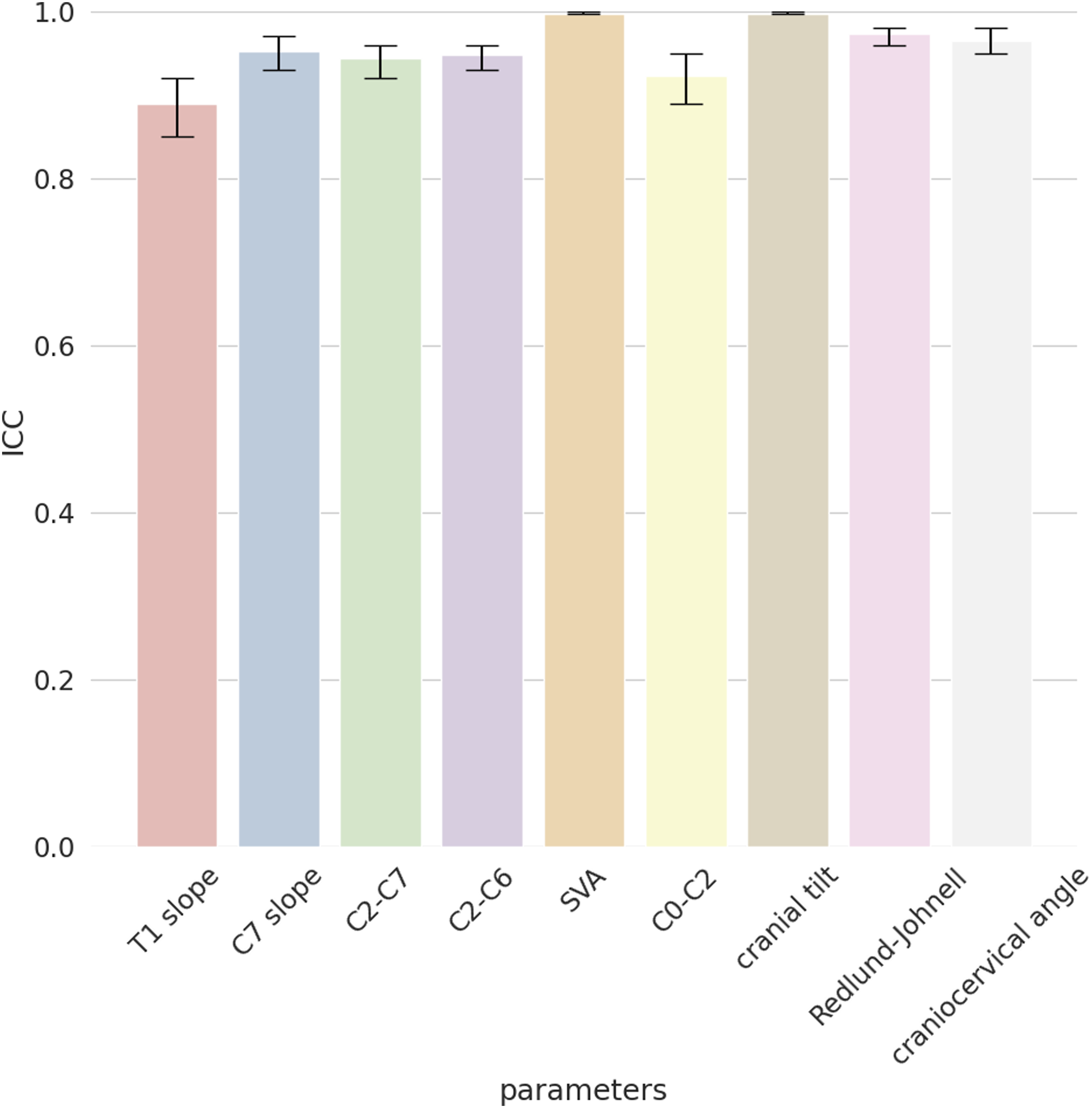

The quantitative evaluation of the performance of the model is here exemplarily reported only for C0-C2 for the sake of brevity. For true values of the angles between 0 and 30 degrees, more than 60% of the model predictions were inside the range of the human annotations (Figure 6), while for higher angles between 30 and 40 degrees 3 out of 8 predictions were correct. Considering a tolerance of 2.5 degrees, almost all the images (76/79) have a correct prediction for C0-C2 (Figure 6). Similar figures were found for the other parameters.

Figure 6.

C0-C2 predictions vs annotations’ range. The y-axes show the percentages of patients, and the x-axes the stratification by ground truth angles values. The chart on the left shows the number of correct predictions that fall inside the annotators’ range while the chart on the right shows the correct predictions considering the annotators’ range expanded with a tolerance of 2.5 degrees. Bars showing the correct predictions are reported in red, and in blue those for the incorrect ones. The numbers at the top of each bar indicate the number of images. For example, for the range 20°-30° there are a total of 34 images: 26 of them (76%) have the predicted C0-C2 correctly classified considering the annotators’ range. If we add the tolerance all 34 images have the parameter correctly classified.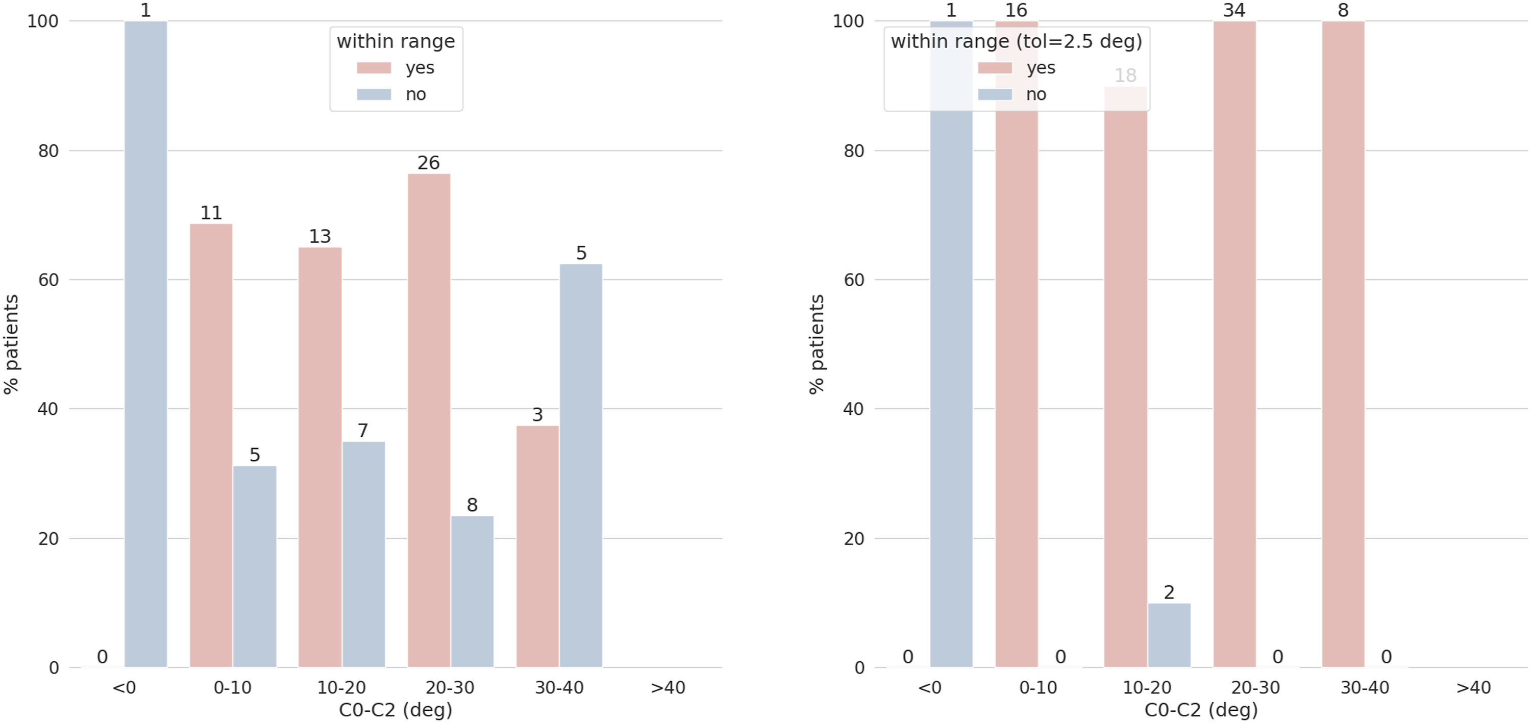

The median errors on the external validation set were generally low for both angles and distances parameters indicating the high robustness and generalization capability of our model (Figure 7). The maximum errors were found for T1 slope, C2-C7, and C2-C6 with values around 8°. For all the angles, the 75th percentiles of the errors were below 4° with the best performances for the CCA with values below 1°. Indeed, regarding the angles, we found median errors of 1.66° (SD 2.46°), 1.56° (1.95°), 2.46° (SD 2.55), 1.85° (SD 3.93°), 1.25° (SD 1.83°), .29° (SD .31°) and .67° (SD .77°) for T1 slope, C7 slope, C2-C7, C2-C6, C0-C2, CT and CCA respectively (Figure 7). As concerns the distances, a generally better performance was observed with a maximum error of around 1.6 mm for SVA and almost all the errors below 1 mm. In detail, we found median errors of .55 mm (SD .47 mm) and .47 mm (.62 mm) for SVA and RJD respectively (Figure 8).

Figure 7.

Boxplot of the angles for the external validation set. The y-axis shows the errors in degrees and the x-axis the name of the angle parameters.

Figure 8.

Boxplot of the distances for the external validation. The y-axis shows the errors in millimeters and the x-axis the name of the distance parameters.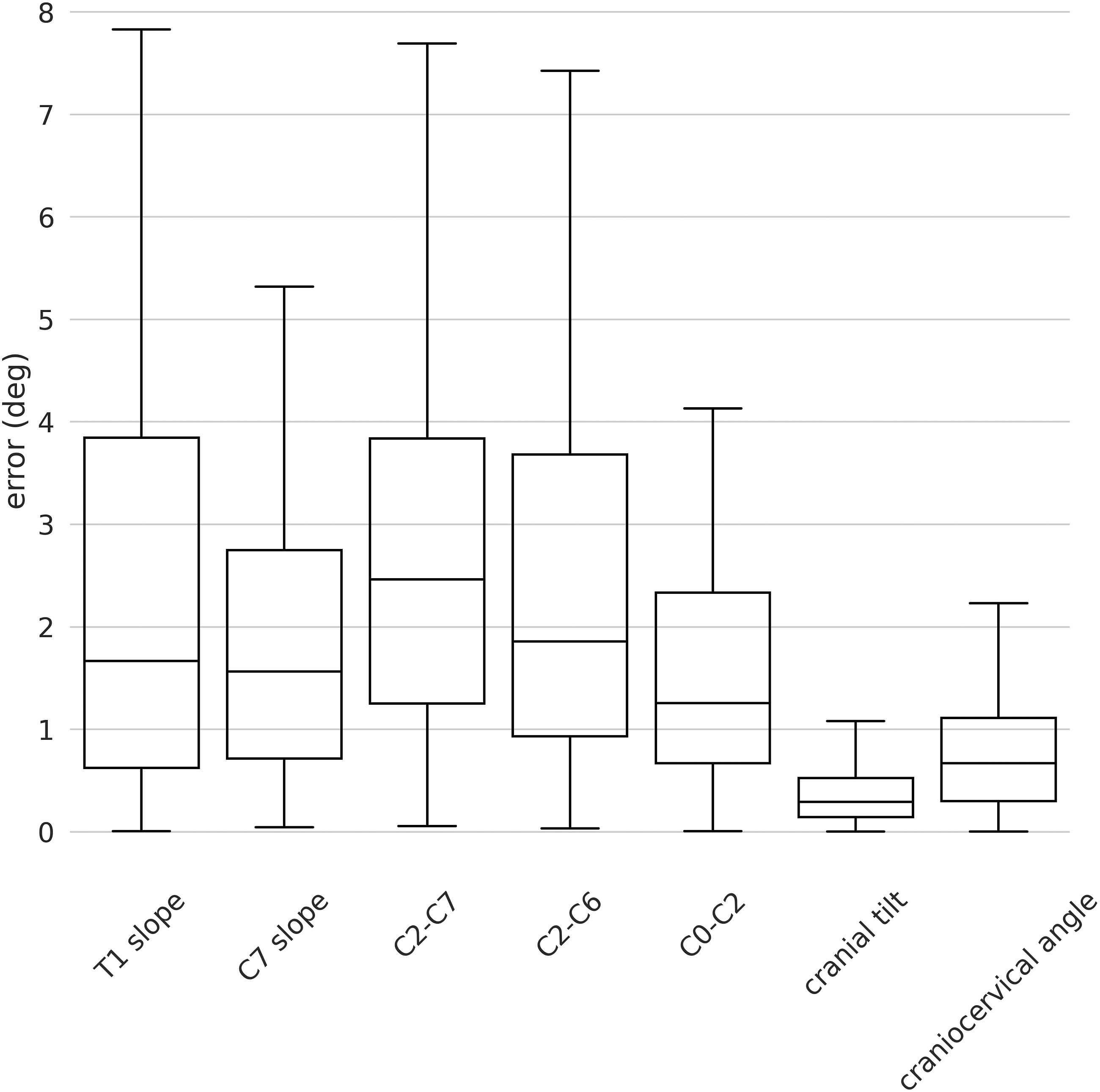

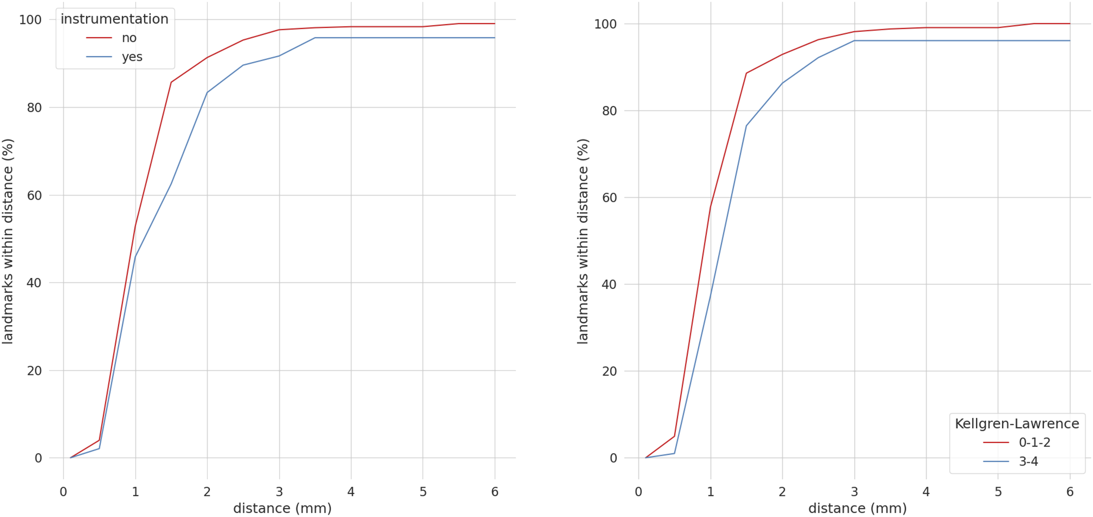
The good performances of our model were confirmed by the high ICC between the model predictions and the ground truth calculated as the mean of the four annotations. In fact, the ICCs were .90 (T1 slope), .94 (C7 slope), .95 (C2-C7), .93 (C2-C6), .98 (SVA), .96 (C0-C2), .99 (CT), .98 (RJD), and .98 (CCA) indicating a high agreement between the model and the annotations (Figure 9). The analysis of the influence of the instrumentation and the degeneration on the model performances shows that there was a slight worsening in case of instrumented or degenerated spines, with a less pronounced effect for degeneration (Figure 10). Considering a threshold distance from the ground truth of 2 mm, more than 80% of the points had a lower localization error both for images with and without instrumentation and for images with and without degeneration. Increasing the threshold to 4 mm, almost all the coordinates were predicted inside the tolerance interval. It can be thus concluded that instrumentation and degeneration only marginally affect the performances of our model.

Figure 9.

ICCs between the model predictions with respect to the average of the annotations. The y-axis reports the ICC values and the x-axis reports the name of the parameters.

Figure 10.

Percentage of correct keypoints obtained stratifying the images in the external validation set based on instrumentation and degeneration. The y-axes show the percentage of correctly predicted landmarks and the x-axes the distance from the ground truth in millimeters considering all 29 points. The red lines indicate the images with no instrumentation (left image) and with no degeneration (right image) while the blue lines the images with instrumentation (left image) and with degeneration (right image).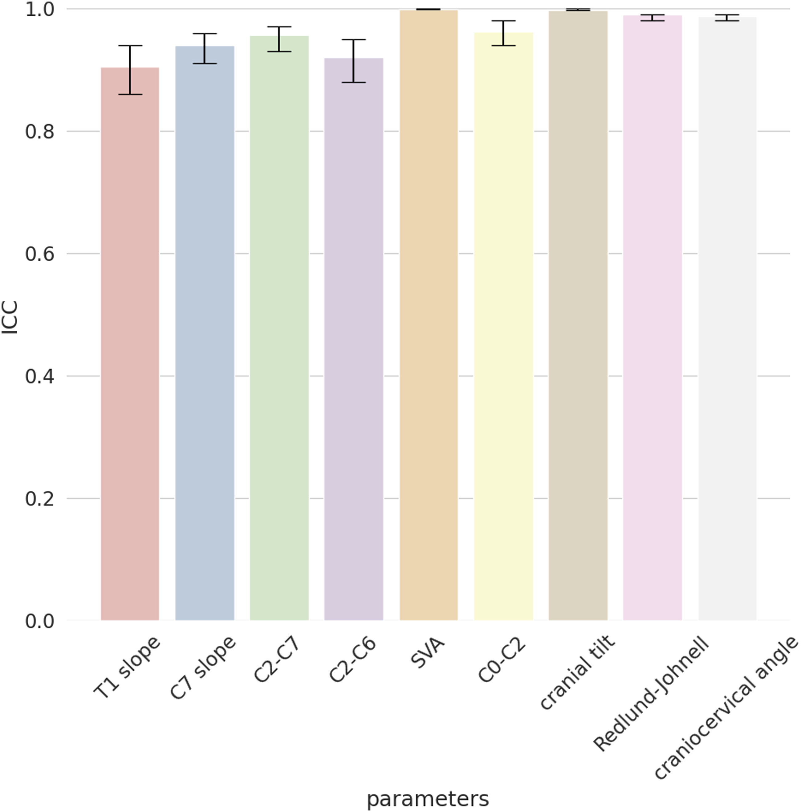

Discussion

We developed a new automated imaging analysis algorithm for measuring cervical spine alignment using a deep learning model. We used 1498 images for training and optimizing the algorithm and tested its performance with 79 images from an external validation dataset annotated by the four examiners. Within the latter dataset, the absolute median errors for the angles calculation were generally lower than 2 degrees, with the exception of C2-C7 (2.46 degrees) (Figure 7), while the median errors for the distances were lower than .55 mm (Figure 8). ICCs between the model predictions and the human annotations exceeded .90 for all the radiological parameters. The presence of instrumentation as well as the degeneration did not seem to affect the model performances much (Figure 10) indicating the high robustness and generalizability of the new tool.

While intra-rater reliability of human raters is inherently limited, automatic image analysis tools show high reproducibility; indeed, the systematic error of the algorithm should be the main point of discussion rather than its intra-rater score. To assess systematic errors in deep learning models, ideally the ground-truth should not be defined by a single human evaluator. However, since there is no golden rule for determining ground truth without human examiners, the best compromise is to define it by combining the observations of more human evaluators. Therefore, the inter-rater reliability between the algorithm and the average of various human raters would be the most appropriate way to assess the accuracy of the model at this time.^13,15-17,22 Several studies have reported the inter-rater reliability of cervical spine alignment parameter measurements in human raters; for example, the ICC of C2-C7 was reported to be .92-.96.^8-10,35 Marques et al reported the inter-rater reliability for T1 slope, SVA, and occipitocervical tilt of .93, .98, and .91 in terms of ICC.⁹ As far as our deep learning model is concerned, the accuracy of the algorithm was .9-.99 in terms of ICCs, which is considered excellent³⁴ and in the same range of an expert human evaluator.

A few studies have reported the automated analysis of cervical spine alignment. Using a deep learning system to automatically measure the degree of cervical lordosis, Shin et al reported ICCs of .974-.993 compared to expert radiologists.²⁰ Similarly, Wang et al reported ICCs of .76-.95 for the Cobb angle at each level using a newly developed model for the automatic detection of cervical landmarks.²¹ With respect to the present work, these models were dedicated to an individual parameter and did not provide a comprehensive measurement of cervical spine alignment. Another study reported ICCs of .83 for C2-C7 and .77 for T1 slope,²² substantially lower than the present results; it should however be taken into account that the published model processed images of the whole trunk rather than of the cervical spine only. Although it is important to evaluate cervical spine alignment as part of the whole spinopelvic alignment, we believe that the present algorithm using lateral cervical spine radiographs has its own clinical relevance since whole-spine radiographs are rarely taken in patients who present with symptoms of cervical origin only. In addition, radiographs of the cervical spine in clinical practice often contain surgical implants and severe degeneration, which may prevent even spine surgeons and radiologists from measuring parameters with confidence. The strength of this study is that it has shown how surgical implants and the degree of degeneration affect the performance of the algorithm and has indicated areas where there is room for improvement before clinical use.

Several limitations associated with the present study warrant mention. First, the datasets included images acquired with different imaging protocols and variable image quality. In addition, approximately 60% of the cervical spine radiographs in our dataset could not be annotated. Marques et al⁹ evaluated 758 cervical spine lateral radiographs and reported that T1 slope was not measurable in 54% due to poor image quality and occipitocervical tilt was not measurable in 43%, consistently with the results here reported. It should be noted that this issue also affects measurements conducted by human operators, and is confirmed by the various attempts of replacing T1 slope with C7 slope, and C2-C7 with C2-C6.^8,36 Second, we showed that degenerative changes have a slight negative effect on the accuracy of the algorithm, but there may be some debate as to which degenerative classification should be used; the KL grade was first reported by Kellgren et al and is widely used as a degenerative assessment in the cervical spine with a reported ICC of .71,^8,37 which can be interpreted as good but not excellent reliability.⁸ Furthermore, the annotation to train the algorithm was performed by a single examiner, as this is a time-consuming task. Given that previous studies have reported excellent inter-rater reliability in measuring cervical spine parameters, the impact of this limitation on the results is expected to be minor.^8,9,35 Finally, we believe that this model should be used as an assisting tool to enhance the speed of human evaluators during spine parameter assessments. In fact, the tool takes one second to evaluate a cervical radiograph while the human annotation could take a few minutes.

Conclusions

With the growing understanding of the value of cervical spine alignment, the development of algorithms using lateral radiographs of the cervical spine will be in great demand in clinical and research settings. Using a deep learning model, we developed a new comprehensive automated tool to accurately measure cervical spine alignment in cervical lateral radiographs. The ICC values were in the range .90-.99, indicating an excellent reliability of our model, at least comparable to those of human evaluators. The model accuracy was marginally affected by the presence of surgical implants and severity of degeneration indicating its high robustness. This study indicates areas for improvement before replacing human evaluators altogether.

Footnotes

Declaration of Conflicting Interests

The author(s) declared no potential conflicts of interest with respect to the research, authorship, and/or publication of this article.

Funding

The author(s) disclosed receipt of the following financial support for the research, authorship, and/or publication of this article: This work was supported by the Author Hiroyuki Nakarai received a 3-months fellowship from AO Spine to support his project at the Schulthess Klinik.

Ethical Statement

ORCID iDs

Hiroyuki Nakarai

Andrea Cina

Alexandra Grob

Tamas F. Fekete

Hans-Joachim Wilke

Notes

References

Ames

Blondel

Scheer

, et al. Cervical radiographical alignment: comprehensive assessment techniques and potential importance in cervical myelopathy. Spine. 2013;38(22 Suppl 1):S149-S160.

Scheer

Tang

Smith

, et al. Cervical spine alignment, sagittal deformity, and clinical implications: A review. J Neurosurg Spine. 2013;19(2):141-159.

Patel

Arutyunyan

Plusch

Vaccaro

Jr Vaccaro

. A review of cervical spine alignment in the normal and degenerative spine. J Spine Surg. 2020;6(1):106-123.

Iyer

Nemani

Nguyen

, et al. Impact of cervical sagittal alignment parameters on neck disability. Spine. 2016;41(5):371-377.

Virk

Niedermeier

Khan

. Adjacent segment disease. Orthopedics. 2014;37(8):547-555.

Schroeder

Boody

Kepler

, et al. Comparing health-related quality of life outcomes in patients undergoing either primary or revision anterior cervical discectomy and fusion. Spine. 2018;43(13):E752-E757.

Izeki

Neo

Takemoto

, et al. The O-C2 angle established at occipito-cervical fusion dictates the patient’s destiny in terms of postoperative dyspnea and/or dysphagia. Eur Spine J. 2014;23(2):328-336. doi:10.1007/s00586-013-2963-6

Côté

Cassidy

Yong-Hing

Sibley

Loewy

. Apophysial joint degeneration, disc degeneration, and sagittal curve of the cervical spine. Can they be measured reliably on radiographs? Spine. 1997;22(8):859-864.

Marques

Granström

MacDowall

Moreira

Skeppholm

Olerud

. Accuracy and reliability of X-ray measurements in the cervical spine. Asian Spine J. 2020;14(2):169-176.

10.

Jackson

Harrison

Robertson

Barker

. Chiropractic biophysics lateral cervical film analysis reliability. J Manip Physiol Ther. 1993;16(6):384-391.

11.

Zhang

Lou

Hill

Raso

Wang

. Automatic cobb measurement of scoliosis based on fuzzy hough transform with vertebral shape prior. J Digit Imaging. 2009;22(5):463-472.

12.

Bailey

Rasoulinejad

. Automated comprehensive dolescent diopathic coliosis assessment using MVC-et. Med Image Anal. 2018;48:1-11.

13.

Galbusera

Niemeyer

Wilke

, et al. Fully automated radiological analysis of spinal disorders and deformities: A deep learning approach. Eur Spine J. 2019;28(5):951-960.

14.

Schwartz

Cho

Tang

, et al. Deep learning automates measurement of spinopelvic parameters on lateral lumbar radiographs. Spine. 2021;46(12):E671-E678.

15.

Orosz

Bhatt

Jazini

, et al. Novel artificial intelligence algorithm: An accurate and independent measure of spinopelvic parameters. J Neurosurg Spine. 2022;37(6):893-901.

16.

Grover

Siebenwirth

Caspari

, et al. Can artificial intelligence support or even replace physicians in measuring sagittal balance? A validation study on preoperative and postoperative full spine images of 170 patients. Eur Spine J. 2022;31(8):1943-1951. doi:10.1007/s00586-022-07309-5

17.

Cina

Bassani

Panico

Luca

Masharawi

Brayda-Bruno

, et al. 2-step deep learning model for landmarks localization in spine radiographs. Scientific Reports 2021;11(1). doi:10.1038/s41598-021-89102-w

18.

Kyrölä

Salme

Tuija

Tero

Eero

Arja

. Intra- and interrater reliability of sagittal spinopelvic parameters on full-spine radiographs in adults with symptomatic spinal disorders. Neurospine. 2018;15(2):175-181. doi:10.14245/ns.1836054.027

19.

Schwartz

Valliani

Arvind

, et al. Identification of anterior cervical spinal instrumentation using a smartphone application powered by machine learning. Spine. 2022;47(9):E407-E414. doi:10.1097/brs.0000000000004172.

20.

Shin

Han

Lee

. Temporal trends in cervical spine curvature of South Korean adults assessed by deep learning system segmentation, 2006-2018. JAMA Netw Open. 2020;3(10):e2020961.

21.

Wang

Huang

Liu

Jiao

Bai

. Multi-input adaptive neural network for automatic detection of cervical vertebral landmarks on X-rays. Comput Biol Med. 2022;146:105576.

22.

Yeh

Weng

Huang

Tsai

Yeh

. Deep learning approach for automatic landmark detection and alignment analysis in whole-spine lateral radiographs. Sci Rep. 2021;11(1). doi:10.1038/s41598-021-87141-x

23.

Lowe

. Distinctive image features from scale-invariant Keypoints. Int J Comput Vis. 2004;60(2):91-110.

24.

Krizhevsky

Sutskever

. Imagenet classification with deep convolutional neural networks. Adv Neural Inf Process Syst. 2012. Published online https://proceedings.neurips.cc/paper/2012/hash/c399862d3b9d6b76c8436e924a68c45b-Abstract.html

25.

Newell

Yang

Deng

. Stacked hourglass networks for human pose estimation. In: Leibe

Matas

Sebe

Welling

, eds. Lecture Notes in Computer Science (including subseries Lecture Notes in Artificial Intelligence and Lecture Notes in Bioinformatics). Springer Verlag; 2016:483-499. doi:10.1007/978-3-319-46484-8_29

26.

Bulat

Tzimiropoulos

. How far are we from solving the 2D and 3D face alignment problem? (and a dataset of 230,000 3D facial landmarks). In: 2017 IEEE International Conference on Computer Vision; October 22 2017; Venice:1021-1030: (ICCV).

27.

Chandran

Bradley

Gross

Beeler

. Attention-driven cropping for very high resolution facial landmark detection. In: 2020 IEEE/CVF Conference on Computer Vision and Pattern Recognition (CVPR); June 19 2020; Seattle, WA:5861-5870: IEEE.

28.

Nibali

Morgan

Prendergast

. Numerical coordinate regression with convolutional neural networks; 2018. arXiv [csCV]. Published online January 23, 2018. https://arxiv.org/abs/1801.07372

29.

Paszke

Gross

Massa

, et al. PyTorch: An Imperative Style, High-Performance Deep Learning Library; 2019. arXiv [csCV]. Published online. https://proceedings.neurips.cc/paper/2019/hash/bdbca288fee7f92f2bfa9f7012727740-Abstract.html Accessed January 11, 2023.

30.

Redlund-Johnell

Pettersson

. Radiographic measurements of the cranio-vertebral region. Designed for evaluation of abnormalities in rheumatoid arthritis. Acta Radiol Diagn. 1984;25(1):23-28.

31.

Lee

Kim

Seo

Suk

Kwack

Son

. The influence of thoracic inlet alignment on the craniocervical sagittal balance in asymptomatic adults. J Spinal Disord Tech. 2012;25(2):E41-E47.

32.

Protopsaltis

Lafage

Vira

, et al. Novel angular measures of cervical deformity account for upper cervical compensation and sagittal alignment. Clin Spine Surg. 2017;30(7):E959-E967.

33.

. Epidemiology of Chronic Rheumatism. Atlas of Standard Radiographs of Arthritis; 1963. Published online https://ci.nii.ac.jp/naid/10016993270/ Accessed January 11, 2023.

34.

Koo

. A guideline of selecting and reporting intraclass correlation coefficients for reliability research. J Chiropr Med. 2016;15(2):155-163.

35.

Harrison

Cailliet

Troyanovich

Janik

Holland

. Cobb ethod or arrison osterior angent ethod. Spine. 2000;25(16):2072-2078. doi:10.1097/00007632-200008150-00011

36.

Tamai

Buser

Paholpak

Sessumpun

Nakamura

Wang

. Can C7 slope substitute the T1 slope? An analysis using cervical radiographs and kinematic MRIs. Spine. 2018;43(7):520-525.

37.

Murakami

Nagata

Hashizume

, et al. Prevalence of cervical anterior and posterior spondylolisthesis and its association with degenerative cervical myelopathy in a general population. Sci Rep. 2020;10(1):10455.

Automatic Calculation of Cervical Spine Parameters Using Deep Learning: Development and Validation on an External Dataset

Abstract

Study design

Objectives

Methods

Results

Conclusions

Keywords

Introduction

Materials and Methods

Datasets

Deep Learning Model

Evaluation

Results

External Validation

Discussion

Conclusions

Footnotes

Declaration of Conflicting Interests

Funding

Ethical Statement

ORCID iDs

Notes

References