Sage Journals: Discover world-class research

Abstract

The objective of this study is to examine the effect of taxes and public debt on economic growth. By using a battery of tests and procedures (including quantile regression and extreme bounds analysis) on a set of cross-sectional data covering 177 countries, we found strong evidence to support the hypothesis that both taxes and public debt retard growth. However, it is demonstrated that reducing the tax rate (particularly the corporate tax rate) has no effect on growth and that the tax burden is the variable that is more relevant to growth. This finding is explained in terms of the proposition that wage and salary earners, who bear the brunt of the tax burden, have a high marginal propensity to consume. This means that reducing the tax rate for the rich and corporations is less effective than reducing the overall tax burden by cutting taxes on the wages and salaries of the middle class.

JEL Classification: O43, O47

Plain Language Summary

The Effect of Tax and Public Debt on Economic Growth

This study investigates how taxes and public debt impact economic growth. By analyzing data from 177 countries, the researchers found strong evidence that both taxes and public debt slow down economic growth. Interestingly, reducing the tax rate, especially for corporations, does not boost growth. Instead, the overall tax burden is more crucial for growth. The study suggests that reducing taxes on wages and salaries of the middle class is more effective than cutting taxes for the wealthy and corporations. This is because middle-class earners are more likely to spend their income, stimulating the economy.

Keywords

economic growth public debt tax burden extreme bounds analysis cumulative density function

Introduction

The effect of taxes on economic growth is a controversial and ideological issue that goes beyond the realm of empirical economics. McBride (2012) argues that “the idea that taxes affect economic growth has become politically contentious and the subject of much debate in the press and among advocacy groups.” The Heritage Foundation, a right-wing think tank, is rather vocal in its support of tax cuts on the grounds that lower taxes boost economic growth. According to the Foundation, “higher tax rates reduce the ability of individuals and firms to pursue their goals in the marketplace and thereby also reduce the level of overall private-sector activity.” The Foundation sees individual and corporate income taxes as “important and direct constraint on an individual’s economic freedom,” with adverse effect on economic growth (Miller et al., 2022).

Since the late 1970s, supply-side economists have been conveying the message that tax cuts stimulate economic growth to such a degree that tax revenue would consequently rise rather than fall. Politicians on the right of the political spectrum capitalized on this proposition and enacted tax cuts. Between 2001 and 2003, a variety of tax cuts were enacted under President George Bush II (commonly referred to as the “Bush tax cuts”) through the Economic Growth and Tax Relief Reconciliation Act of 2001, and the Jobs and Growth Tax Relief Reconciliation Act of 2003. This course of action had its supporters (including the Heritage Foundation) but it also triggered significant opposition, most notably from 450 economists (including ten Nobel Prize laureates) who signed a statement opposing the Bush tax cuts. They expressed the view that the tax cut plan proposed by President Bush was not the answer to the problems of jobless growth and rising unemployment, and that the proposed tax cuts would lead to fiscal deterioration that would reduce the capacity of the government to finance investment in schools, health, infrastructure, and basic research, all of which have a strong effect on growth.

However, little empirical evidence supports the hypothesis that tax cuts boost growth, let alone that they pay for themselves. In a study of the Joint Committee on Taxation (2005) that examined the economic effects of reducing marginal tax rates, it is suggested that “growth effects eventually become negative … because accumulating federal government debt crowds out private investment.” The study concludes that “lowering marginal tax rates is likely to harm the economy over the long run if the tax reductions are deficit financed.” In June 2012, a survey was conducted whereby experts were asked if a cut in federal income tax rates in the US would raise taxable income enough so that the annual total tax revenue would be higher within 5 years than without the tax cut. No one ticked the “Strongly Agree” or “Agree” boxes, but 71% ticked the “Strongly Disagree” or “Disagree” boxes (Chicago Booth, 2012).

A related issue is the effect of public debt on economic growth. These two factors (taxes and debt) are rarely considered together, even though they are related, in the sense that raising taxes and accumulating public debt are two alternative means of financing the budget deficit (in addition to the hazardous act of financing the deficit by monetizing it). Gale and Samwick (2014) identify the link by suggesting that the effect of a tax cut depends on whether it is or is not financed by reduced expenditure. If it is not, public debt will accumulate and if debt is bad for economic growth, then tax reduction is indirectly conducive to decelerating growth.

The question is whether or not excessive debt is harmful. It is widely believed that a moderate level of debt that is used to finance productive projects is useful whereas excessive debt can be rather harmful, particularly if it is used to finance unproductive activity, such as military spending. The Economist (2010) goes as far as describing public debt as a “Ponzi scheme that requires an ever-growing population to assume the burden—unless some dues ex machine, such as a technological breakthrough, can boost growth.” However, Reinhart and Rogoff (2009) argue that the danger threshold is 90% of GDP, even though they suggest that “seldom do countries simply ‘grow’ their way out of deep debt burdens.”

One way to evaluate the proposition that higher tax rates have a negative effect on economic growth is to examine the relation between tax rates and economic growth over time. If high taxes are bad for the economy, we should expect robust economic growth during periods characterized by low tax rates, and vice versa. The corresponding cross-sectional argument is that if high taxes are bad for economic growth then, ceteris paribus, countries with high tax rates should experience slower growth than those with low tax rates. The same arguments can be made for the effect of public debt on economic growth. This study is motivated by the desire to provide evidence for the effect of taxes and public debt on growth—more specifically, to find out if countries with high taxes and/or large public debt experience slow growth compared with countries that have low taxes and/or small public debt.

The problem here is that econometrics and ideology can be a lethal combination, in the sense that econometric analysis can be used to produce results that confirm prior beliefs. This is particularly the case with cross-sectional regressions that contain a large number of explanatory variables, because different combinations of explanatory variables invariably produce different results. Young and Holsteen (2017) argue that theory rarely says which variables should appear in the model, suggesting that “theory can be tested in many different ways and modest differences in methods may have large influence on the results.” The search for “good” results makes it tantalizing to indulge in data mining, involving the estimation of thousands of regression equations and reporting the most appealing one or few. Gilbert (1986) argues on similar grounds, suggesting that published results are accepted because the reported regression equation has coefficients that are correctly signed and statistically significant. However, he notes that these significant coefficients cannot be taken as evidence for or against the hypotheses under investigation, wondering about the other 999 regressions assigned to the bin.

The objective of this paper is to investigate the effects of taxes and public debt on economic growth using cross-sectional data covering 177 countries and a large number of variables that are believed to be consequential for growth. To overcome the problem of the tendency to report desired results by indulging in data mining and reporting one “nice-looking” regression equation, we employ extreme bounds analysis (EBA) in which inference is based not on the estimated point values of the coefficients but rather on the distribution of the coefficients obtained by estimating a large number of equations specified systematically according to a strict procedure.

This paper makes significant contributions to the literature on a controversial issue in public finance. The first contribution is methodological, as the methodology used in this paper overcomes the model uncertainty problem that makes the underlying model subject to the Leamer (1983) critique. Invariably, all previous studies are subject to the Leamer critique because the results are derived from one equation following heavy data mining. The second contribution is that it deals with an important question in public finance, which is whether or not it is a good idea to cut taxes and finance the resulting deficit by borrowing. This issue is tackled by specifying and estimating a model in which growth is a function of both taxes and public debt. Furthermore, this study identifies the best variable to represent the effect of taxes, which is the tax burden rather than either the corporate or personal income tax rate. Last, but not least, this study sheds some light on the “trickle-down effect,” the (blunt) proposition that cutting taxes for the rich benefits the poor. This is particularly the case when tax cuts are financed by borrowing, which produces a negative net effect on growth. Conservative politicians often talk about, and sometimes they implement policies aimed at, boosting growth through tax cuts for the rich, which is not a good idea as the results of this study shows.

Literature Review: The Effect of Taxes on Economic Growth

We start with the literature review of the effect of taxes on economic growth by considering the studies that came out in reaction of the Bush tax cuts. Kogan (2003) evaluated the claims that the Bush tax cuts of 2001 would boost growth and found that “these tax cuts would have only a small effect on the economy over the long term,” and that “the effect is as likely to be negative as positive.” On the same issue, the CBO (2001) concluded that “the cumulative effects of the new tax law on the economy are uncertain but will probably be small.”Gale and Potter (2002) found that the effect on long-term economic growth was more likely to be a small negative than a small positive. Elmendorf and Reifschneider (2002) concluded that “a sustained tax cut reduces output [GDP] in the long run and raises output by less than 50 cents per dollar of tax reduction in the short run.”Auerbach (2002) found that “in the long run, the level of capital and hence output [GDP] has been permanently reduced by the prolonged period of reduced national saving induced by the tax cut [because of the tax cut’s effect in swelling budget deficits].”Ruffing and Horney (2010) dispute a report of the Heritage Foundation (Reid, 2010) claiming that the tax cuts initiated by George Bush II are not a significant factor behind the deficits. In particular, they argue that the analysis ignores the fact that rapidly-rising interest payments result in significant part from the tax cuts.

Many studies have demonstrated determintal effect of tax cuts on economic growth. For instance, Aaron et al. (2004) found that “historical evidence shows no clear correlation between tax rates and economic growth” and that “comparisons across countries confirm that rapid growth has been a feature of both high- and low-tax nations.”Allard and Lindert (2006) show that at levels of taxation at or even significantly above those now seen in the US, increasing the ratio of tax revenue to GDP leads to an improvement in economic performance. They explain this result by noting that the additional revenues raised by higher-tax countries are frequently used to undertake growth-promoting activities such as investment in public education, infrastructure, and public health. Mazerov (2010) argue that “corporate income tax cuts are unlikely to have a positive impact on a state’s rate of economic growth or the pace at which it generates private-sector jobs.” The CBO (2008) concludes that “a general cut in business tax rates will tend to generate significantly less investment demand for each dollar of [lost] revenue than a cut that applies only to new investment.” Likewise, the CRS concludes that “most evidence does not suggest that business tax cuts would provide significant short-term stimulus” (Gravelle et al., 2009).

A more recent review of the literature by the Tax Foundation was published in 2021, in which it is reiterated that “taxes, particularly on corporate and individual income, harm economic growth” (Durante, 2021). In his review, Durante identifies methodological challenges, such as failure to control for other factors that impact economic growth, the difficulty of distinguishing between short-run and long-run impact, and whether a tax policy change represents a net tax increases or decrease. In particular, Durante refers to the meta-study of Alinaghi and Reed (2021) of 979 estimates from 49 studies and finds that a 10% tax cut boosts GDP growth by 0.2%. Other supportive studies include Mertens and Montiel Olea (2018), Zidar (2019), Ljungqvist and Smolyansky (2018), Gunter et al. (2019), Nguyen et al. (2021), and Cloyne et al. (2018).

The same criticism of the Tax Foundation’s 2012 paper is applicable to the 2021 paper: it is a literature survey designed to confirm the prior belief that taxes are bad for economic growth. Gale and Samwick (2014) suggest that the net impact on growth of a cut in individual income tax rate cut is uncertain, arguing that many estimates suggest that it is either small or negative. They find that “it is by no means obvious, on an ex ante basis, that tax rate cuts will ultimately lead to a larger economy.”Husak (2021) sees “no obvious relationship between top tax rate and economic growth in the US” and that “over time, high top rates are associated with higher economic growth.”Jaimovich and Rebelo (2017) find that “low tax rates have a very small impact on long-run growth rates.”Hoang et al. (2021) note that “taxes on goods and services promote economic growth in rich countries.” Hope and Limberg (2021) suggest that tax cuts do not have any significant effect on economic growth and conclude that their results provide strong evidence against the “influential political–economic idea” that tax cuts for the rich “trickle down” to boost the wider economy. Milasia and Waldmann (2018) find that the marginal effect of higher top tax rates becomes negative above a growth-maximizing tax rate in the order of 60%. The meta-analysis conducted by Gechert and Heimberger (2022) leads to the “ambiguous conclusion” that corporate tax cuts may boost, reduce, or do not significantly affect growth. As a matter of fact, they cannot reject the hypothesis of a zero effect of corporate taxes on growth.

The evidence on this or any issue should be judged not only in terms of the numbers coming out of a computer but also in terms of theory and common sense. There are some good reasons to believe that tax cuts do not necessarily boost economic growth. Mazerov (2010) puts forward a number of arguments to support this conjecture by suggesting that tax cuts (i) would produce no net short-term stimulus, due to state balanced-budget requirements; (ii) could lead to a near-term drop in total in-state economic activity because corporations are unlikely to spend the full amount of the tax cut in-state; (iii) would create little or no added incentive for corporate investment in the long run; (iv) could adversely affect long-term growth by leading to cuts in public services; and (v) are not rooted in real-world economic success stories. On the “pay for themselves” proposition, Mazerov argues that “the small economic impacts of state corporate tax cuts and the large loss of revenue mean that such cuts do not stimulate enough new taxable economic activity—and thus enough new revenues—to fully offset the revenues lost from the tax cut.”

Literature Review: The Effect of Public Debt on Growth

Economists have identified several macroeconomic channels through which debt can impact economic growth adversely. High public debt exerts a negative effect on the accumulation of capital, and consequently economic growth, via rising long-term interest rates, higher distortionary tax rates, inflation, and a general constraint on countercyclical fiscal policies. Since the advent of the global financial crisis of 2007 to 2008, and the subsequent European sovereign debt crisis beginning in late 2009, economists have been exploring the effect of government debt on economic growth. In 2010 Carmen Reinhart and Kenneth Rogoff published their highly-cited paper “Growth in a Time of Debt,” which has become influential among commentators, academics and politicians in the debate on austerity and fiscal policy in debt-burdened economies (Reinhart and Rogoff, 2010).

The adverse consequences of excessive public debt have been identified by the Congressional Budget Office (CBO, 2010). The first is that a growing portion of private savings would be used to finance the acquisition of government securities rather than to finance investment in productive capital goods and job creation ventures. Some observers have warned that this is conducive to non-job creating growth in some government activities at the expense of the productive sectors of the economy (e.g., Friedman, 2002). Then there is the traditional argument that rising public debt results in higher interest rates and competition between the public sector and private sector for loanable funds, forcing a crowding out of private sector investment, which adversely affects growth and employment. Rising interest costs force reductions in important government programs that contribute to the development of human capital.

A study of the Bank for International Settlements, which warns of the hazards of accumulating debt, identifies three serious consequences of excessive public debt (Cecchetti et al., 2010). The first is that investors demand a higher risk premium for holding the bonds issued by heavily indebted countries. The second is that a higher level of public debt implies that a significant amount of resources is allocated to debt service, which will eventually require high taxes. The third is that a high debt burden is likely to reduce the size and effectiveness of fiscal response to an adverse shock.

A question that often arises concerns the “danger” level of debt. Reinhart and Rogoff (2009) argue that the danger level is 90% of GDP. In a testimony to the US Senate, Reinhart (2010) noted that high debt/GDP levels (90% and above) are associated with notably lower growth outcomes. This characterization of the danger level of debt is not accepted by economists across the board. For example, Krugman (2010) disputes the existence of a solid debt threshold or danger level, arguing that “low growth causes high debt rather than the other way around.”Bernanke (2010) also disputes the presence of a debt threshold, arguing that neither experience nor economic theory clearly indicates the threshold at which government debt begins to endanger prosperity and economic stability. However, he goes on to warn that “given the significant costs and risks associated with a rapidly rising federal debt, our nation should soon put in place a credible plan for reducing deficits to sustainable levels over time.” The CBO (2010) makes the same point by suggesting that the tipping point for a crisis does not depend solely on the debt to GDP ratio and that other important factors do matter, such as the long-term budget outlook, near-term borrowing needs and the health of the economy.

In general, it has been found that a high level of public debt to GDP is detrimental to economic growth. Calderón and Fuentes (2013) argue that the growth prospects of a nation are stymied by the burden of government debt and reveal, by using a large set of panel data, a negative and robust effect of public debt on growth. Heimberger (2021) conducts a meta-analysis of 826 estimates from 48 primary studies and finds that a 10 percentage point increase in public-debt-to-GDP is associated with a decline in annual growth rates by 0.14 percentage points. de Rugy and Salmon (2020) note that the empirical evidence overwhelmingly supports the view that a large amount of government debt has a negative impact on economic growth potential, such that the impact gets more pronounced as the level of debt rises. Salmon (2021) reviews recent studies and reaches the conclusion that high levels of public debt have a negative impact on economic growth. By using quantile regression, San and Chin (2023) reach the same conclusion and note that “government debt negatively affects economic growth across all the quantiles.”

It is worthy to note that the effects of taxes and public debt on economic growth are typically examined separately, even though they are related because they are alternative means of financing the budget deficit. Those who believe that both taxes and public debt harm growth may face a problem of reconciliation. If taxes are cut to boost growth, the budget deficit will have to be financed by more borrowing, leading to the accumulation of more public debt. If debt is bad for economic growth and the accumulation of more debt results from cutting taxes, then lower taxes must be bad for growth, unless tax reduction is matched by lower expenditure. If expenditure is non-discretionary, then it cannot be reduced, in which case reduced taxes must be accompanied by the accumulation of debt. This is probably why the results show that the effect of debt on growth is more conspicuous than the effect of tax cuts.

Model Specification and the Choice of Explanatory Variables

Model specification, as described in this section, is intended to answer the research question addressed in this study, which is whether or not taxes and public debt have negative effects on economic growth. Since economic growth depends on variables other than taxes and public debt, other potential determining variables are considered, which allows us to test various hypotheses on the effects exerted by potential determining variables on economic growth. However, based on the literature review presented forward, the focus is on two hypotheses pertaining to the effects of taxes and public debt on economic growth as follows:

H₁: Higher taxation is negatively associated with economic growth.

H₂: Higher public debt is negatively associated with economic growth.

The model is specified such that the dependent variable is the growth rate, measured as the percentage change in real GDP over a year or the average of more than 1 year, whereas the explanatory variables are potential determinants of growth, which are numerous. The very basic cross-sectional growth model represents the catch-up hypothesis whereby countries with low GDP per capita grow faster than those with high GDP per capita (hence, low-income countries catch up with high-income countries in the long run). One reason why low income per capita countries grow faster than those with high income per capita is that it takes a small absolute change to produce a high percentage change in GDP. For a survey of the literature on the catch up hypothesis, see Johnson and Papageorgiou (2020). A cross sectional regression that represents the catch up hypothesis can be written as

Y = α + γ_{0} X_{0} + ε

(1)

where Y is GDP growth rate and $X_{0}$ is GDP per capita. Naturally, economic growth is determined by more than the current level of GDP per capita, in which case a generalized model can be written as

Y = α + γ_{0} X_{0} + \sum_{i = 1}^{m} γ_{i} X_{i} + ε

(2)

where $X_{i}$ is any of m variables (in addition to GDP per capita) that determine the growth rate.

In this exercise the set of m explanatory variables includes the 15 variables listed in Table 1. These variables are divided into three groups, the first of which contains four variables that represent taxes and public debt. “INCOME TAX RAT,”“INCOME TAX RAT,” is the personal income tax rate, “CORPORATE TAX RAT,” is the corporate tax rate, “TAX BURDE,” is the tax burden, and “PUBLIC DEBT” is public debt as a percentage of GDP. A question arises here as to the validity of including taxes and debt as separate explanatory variables. The specification is valid because taxes and debt represent two alternative ways of financing government spending but they affect growth through different channels, as explained earlier. The interaction of the two variables with respect to economic growth is identified in a study of the Joint Committee on Taxation (2005) where it is suggested that the effect of tax cuts on growth becomes negative eventually because the consequent accumulation of public debt crowds out private investment.

Table 1.

Variable Description and Measurement.

Type	Variable	Description
Dependent variables	Annual GDP Growth Rate (%)	Annual percentage change of real GDP measured at constant prices (latest available)
Dependent variables	5 Year GDP Growth Rate (%)	Average growth rate measured over the last 5 years when data are available
Independent variables	GDP per capita (PPP)	GDP converted into dollar at PPP exchange rates divided by total population
	Income Tax Rate (%)	Tax rate on individuals’ taxable income
	Corporate Tax Rate (%)	Tax rate on corporate taxable income
	Tax Burden (% of GDP)	Overall tax burden from all forms of taxes as a percentage of GDP. It includes direct and indirect taxes imposed by all levels of government
	Public Debt (% of GDP)	Gross government debt as a percentage of GDP, which is a measure of the cumulative total of all government borrowings less repayments that are denominated in a country’s currency
	Government Expenditure (% of GDP)	Government expenditure includes consumption by the state and all transfer payments related to various entitlement programs
	Inflation (%)	Annual percentage change in consumer prices
	Property Rights (index, 0-100)	A measure of the extent to which a country’s legal framework allows individuals to acquire, hold, and utilize private property and the extent to which these rights are secured by clear laws that the government enforces effectively
	Judicial Effectiveness (index, 0–100)	Average score for judicial independence, quality of the judicial process, and perceptions of the quality of public services and the independence of the civil service
	Government Integrity (index, 0–100)	Average score for the perceptions of corruption, risk of bribery, and control of corruption
	Business Freedom (index, 0–100)	Average score for access to electricity, business environment risk, regulatory quality, and women’s economic inclusion
	Labour Freedom	A measure of the legal and regulatory framework of a country’s labour market, including regulations concerning minimum wages, associational rights, laws inhibiting layoffs, severance requirements, and measurable regulatory restraints on hiring and hours worked
	Monetary Freedom (index, 0–100)	The index combines a measure of inflation with an assessment of various government activities that distort prices
	Trade Freedom (index, 0–100)	A composite measure of the extent of tariff and non-tariff barriers that affect the imports and exports of goods and services
	Investment Freedom (index, 0–100)	A measure of regulatory restrictions that are typically imposed on investment
	Financial Freedom (index, 0–100)	An indicator of banking efficiency and a measure of independence from government control and interference in the financial sector

The second group contains two variables that are believed to affect growth: “GOVERNMENT EXPENDITUR,” which is government expenditure as a percentage of GDP, and “INFLATIO,” which is the inflation rate. The third group contains components of the Heritage Foundation’s economic freedom index: “PROPERTY RIGHT,” is property rights, “JUDICIAL EFFECTIVENES,” is judicial effectiveness, “GOVERNMENT INTEGRIT,” is government integrity, “BUSINESS FREEDO,” is business freedom, “LABOUR FREEDO,” is labor freedom, “MONETARY FREEDO,” is monetary freedom, “TRADE FREEDO,” is trade freedom, “INVESTMENT FREEDO,” is investment freedom, and “FINANCIAL FREEDO,” is financial freedom. Miller et al. (2022) provide a detailed description and these indices.

The inclusion of government expenditure and inflation in the set of explanatory variables can be justified easily. Government expenditure is viewed by the Heritage Foundation as being “harmful to economic freedom,” which makes it harmful to economic growth. The underlying rationale is that government expenditure has to be financed by a higher level of taxation and entails an opportunity cost, which is the value of the consumption or investment that would have occurred had the resources involved been left in the private sector. The Foundation believes that “even if an economy achieves faster growth through more government spending, such economic expansion tends to be only temporary, distorting the market allocation of resources and private investment incentives” (Miller et al., 2019). Whether government expenditure boosts or retards growth depends on where the expenditure goes; spending on health, education, and infrastructure is bound to be conducive to growth (Abu Alfoul et al., 2024a, 2024b). This means that it is the type, not the volume, of government expenditure that matters.

Inflation is widely expected to exert a negative impact on economic growth. To start with, inflation provides a disincentive to saving, which is a source of the financial resources used to finance capital accumulation. The uncertainty associated with high and volatile unanticipated inflation has been found to be one of the main determinants of the rate of return on capital and (Bruno, 1993; Pindyck & Solimano, 1993). Even fully anticipated inflation may reduce the rate of return on capital, as revealed by Jones and Manuelli (1993) and Feldstein (1996). Inflation also affects other determinants of growth such as human capital and investment in R&D. Inflation worsens long-run macroeconomic performance by reducing the efficiency with which factors are used. In the extreme case of hyperinflation, a total economic collapse is inevitable (see, e.g., Moosa, 2014). On the other hand, Bruno and Esaterly (1996) suggest that “like a bickering couple, inflation and growth just cannot seem to decide what their relationship should be.” They find no evidence for any relation between inflation and growth when the inflation rate is less than 40% (their definition of high inflation).

The rest of the variables are indices of the components of economic freedom as prepared and reported by the Heritage Foundation (Miller et al., 2019, 2022). The Heritage Foundation has no doubt that “there is a robust relationship between improvements in economic freedom and economic growth” and that “the relationship between gains in economic freedom and rates of economic growth is consistently positive.” More specifically, the Foundation reports that the economic growth rates of countries where economic freedom has expanded the most are at least 30% higher than those of countries where freedom has stagnated or slowed.

Estimation Methodology

Straight cross-sectional regressions with a large number of explanatory variables are problematic because they are subject to the Leamer (1983) critique that the results are sensitive to the selected set of explanatory variables. The underlying exercise becomes something like a fishing expedition, involving intensive specification search, until the “right” results are obtained. This is particularly convenient for those who aspire to results that confirm prior beliefs, which is invariably the case with respect to work on this particular topic.

This problem arises because theory is not adequately explicit about what variables that should appear in the “true” model. To circumvent this problem, Leamer (1983, 1985) suggested the use of extreme bounds analysis (EBA) to find out if the determinants of the dependent variable are robust, in which case the researcher would look for robustness as opposed to statistical significance. By calculating upper and lower bounds of the coefficient on the variable of interest from all possible combinations of potential explanatory variables, it is possible to assess the sensitivity of the estimated coefficients to specification changes.

EBA is based on a linear regression of the form

Y = α + γ_{0} X_{0} + β Q + \sum_{i = 1}^{k} γ_{i} Z_{i} + ε

(3)

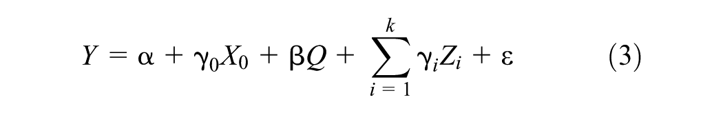
where “GDP PER CAPIT,” is the free variable that is always included in the regression because its importance has been established by previous studies (and because it makes sense theoretically or at least intuitively), Q is the variable whose robustness is under consideration (the variable of interest), and is a potentially important variable, such that each the number of Z variables in each estimated equation is k. If $X = {X_{1}, X_{2}, \dots X_{m}}$ , then $Q ϵ X$ and $Z ϵ X$ such that $Q \neq Z$ .

The procedure involves varying the set of Z variables to find the widest range of coefficients on the variable of interest, β, that standard tests of significance do not reject. If the extreme (minimum and maximum) values remain significant and of the same sign, one can infer that the result (and hence, the variable of interest) is “robust.” Otherwise, the variable is “fragile.” In other words, for a variable of interest to be robust, $β_{\min}$ and $β_{\max}$ must be significant and of the same sign. Since the number of Z variables in this exercise is 14, and at any one time three Z variables are included in the regression, the number of regressions that have to be run for each variable of interest is 364, which gives a total of 5460 regressions. Specifically, the number of regressions per variable of interest is calculated as 14! ((3! × 11!) = 364). The total number of regressions is 364 × 15 = 5460.

Sala-i-Martin (1997) suggests a refinement of the procedure by departing from the labeling of variables as robust and fragile, opting instead to examine the entire distribution of β. Specifically, his procedure is based on the fraction of the probability density function lying on each side of zero, Cumulative Density Function-CDF (0). Thus, if 95% of the density function lies to the right or left of zero, the underlying variable is considered “Robust”; otherwise, it is deemed “Fragile.” The cumulative distribution function is calculated from the weighted average of the point estimates of β where the weights are integrated likelihoods. The CDF is computed under the assumptions of normality and non-normality of the distribution of the estimated. In this exercise, the CDF is calculated under normality and otherwise (general distribution). Hence, Leamer’s (1985) form of EBA is highly restrictive, as it classifies a variable as fragile if even one model specification produces an opposite sign or insignificant result. In contrast, Sala-i-Martin’s (1997) form of EBA evaluates the entire distribution of coefficients and deems a variable robust if most (e.g., CDF ≥ %) of the estimates lie on the same side of zero, making it less restrictive and widely applicable in empirical research (Khatatbeh, 2019; Khatatbeh & Moosa, 2022).

Data and Preliminary Results

The sample data, obtained from “the Heritage Foundation,” covers cross-sectional data of 177 countries. The countries were selected based on the availability of data, whereas the Heritage Foundation database comprises data for 184 countries, with the remaining countries excluded due to missing observations. The variables, definitions, and measurement can be found in Table 1. Two growth variables are used: the 1-year growth (latest available observation) and 5-year average growth (calculated from the last available annual observations, e.g., 2017–2021).

The starting point is to look at the rank correlation between the two growth rates and the tax and debt variables. The rank correlation coefficients are reported in Table 2 with the p-values placed in square brackets. We can see that while the two tax rates are insignificantly correlated with growth rates, the tax burden has a significantly negative correlation with both growth rates. This suggests that growth is influenced less by the statutory tax rate and more by the actual tax burden, particularly in systems where wage and salary earners—who typically have a high marginal propensity to consume—shoulder a disproportionate share relative to their incomes. Significantly negative correlation can be observed between public debt and the average 5-year growth rate.

Table 2.

Rank Correlation between Growth Rates and Tax/Debt Variables.

Variables	Annual GDP growth rate annual GDP growth rate	5-year GDP growth rate
Income Tax Rate	0.09 [0.21]	−0.14* [0.06]
Corporate Tax Rate	−0.04 [0.57]	0.04 [0.57]
Tax Burden	−0.16** [0.03]	−0.37*** [0.00]
Public Debt	−0.09 [0.23]	−0.21** [0.01]

Note. p-Values are reported in square brackets. The asterisks ***, **, * identify significance at the 1%, 5%, and 10%, respectively.

An alternative to correlation is to split the variables into high and low groups, where high is defined by the values above the 66th percentile and low is defined by the values below the 33rd percentile. Having done that, it is possible to calculate the percentage of countries falling in one of four groups: HH (high growth and high tax/debt), LL (low growth and low tax/debt), HL (high growth and low tax/debt) and LH (low growth and high tax/debt). If growth is negatively related to tax/debt, then more countries must fall in the HL and LH groups than in the HH and LL groups.

Table 3 reports the percentages out of the total sample of 177 countries. We can see that, particularly for the 5-year growth rate, more countries fall in the HL and LH cells than those falling in the HH and LL cells. In Table 4, we can see examples of the countries in each cell. Consider, for example, the effect of the tax burden, “TAX BURDEN,” on the 5-year growth rate. Bolivia and Iceland have high growth and high tax burden, Kuwait and Lebanon have low growth and low tax burden, India and Malawi have high growth and high tax burden, and Brazil and France have low growth and high tax burden. With respect to public debt, we can see that Egypt has high growth and high public debt whereas Estonia has low growth and low public debt. Conversely, Bulgaria has high growth and low public debt, while Canada has low growth and low public debt.

Table 3.

Percentage of Countries Falling in High/Low Groups.

	Annual GDP growth rate				5-year GDP growth rate
Variables	HH	LL	HL	LH	HH	LL	HL	LH
Income tax rate	6.2	13.6	15.8	10.7	6.2	9.6	14.7	13.0
Corporate tax rate	12.4	10.7	10.2	13.0	14.1	10.2	7.3	10.7
Tax burden	6.8	9.6	14.1	13.6	4.5	6.8	17.0	17.5
Public debt	9.0	11.3	13.0	12.4	9.6	7.9	14.1	16.4

Note. HH = high growth, high tax/debt; LL = low growth, low tax/debt; HL = high growth, low tax/debt; LH = low growth, high tax/debt.

Table 4.

Examples of Countries in High/Low Groups.

Variables	HH	LL	HL	LH
Annual GDP growth rate
Income tax rate	China Guinea	Afghanistan Azerbaijan	Bangladesh Bolivia	Belgium Chad
Corporate tax rate	India Kenya	Belarus Germany	Cambodia Czech Republic	Australia Brazil
Tax burden	Bolivia Estonia	Lebanon Nigeria	Burma Ethiopia	Australia Barbados
Public debt	Bhutan Ghana	Botswana Denmark	Burma Latvia	Belgium Brazil
	HH	LL	HL	LH
5-Year GDP growth rate
Income tax rate	Benin Costa Rica	Jamaica Liberia	Botswana Dominican	Austria Denmark
Corporate tax rate	Burma Cameroon	Belarus Canada	Bahrain Maldives	Egypt Venezuela
Tax burden	Bolivia Iceland	Kuwait Lebanon	India Malawi	Brazil France
Public debt	Egypt Ghana	Estonia Haiti	Bulgaria Indonesia	Belgium Canada

Note. HH = high growth, high tax/debt; LL = light growth, low tax/debt; HL = high growth, low tax/debt; LH = low growth, high tax/debt.

As stated earlier, support for the proposition that growth is negatively related to taxes and public debt is indicated by more countries falling in the HL and LH cells than those falling in the HH an LL cells. Table 5 reports the percentages of countries falling in the combined HH+LL and HL+LH cells with the $z_{α}$ statistic for the difference between two proportions (a 5% critical value of 1.96, since it follows a normal distribution). We can see that in all cases, the number of countries falling in the HL+LH group is higher than the number of those falling in the HH+LL cells; the only exception being the effect of corporate income tax on the 5-year growth rate. What matters, however, is the statistical significance of the difference, which is indicated by the rejection of the null hypothesis of the equality of the two proportions when $| z_{α} | > 1.96$ . Significant differences are clear in the case of the 5-year growth rate, implying some evidence that the reduction in personal (but not corporate) income tax rate, tax burden, and public debt is conducive to growth.

Table 5.

Testing the Difference Between Ratios.

	Annual GDP growth rate			5-Year GDP growth rate
Variables	HH+LL	HL+LH	$z_{α}$	HH+LL	HL+LH	$z_{α}$
Income Tax Rate	19.8	26.5	−1.50	15.8	27.7	−2.74
Corporate Tax Rate	23.1	23.2	−0.02	24.3	18.0	1.45
Tax Burden	16.4	27.7	−2.58	11.3	34.5	−5.40
Public Debt	20.3	25.4	−1.14	17.5	30.5	−2.89

Note. HH = high growth, high tax/debt; LL = low growth, low tax/debt; HL = high growth, low tax/debt; LH = low growth, high tax/debt.

Quantile Regression Results

Additional evidence can be obtained by running exploratory quantile regressions of growth on the tax and public debt variables. In a quantile regression, the conditional quantiles of a dependent variable are expressed as a linear function of the explanatory variables, where the quantiles can be the medians or otherwise. Quantile regression, which is better at dealing with outliers, is used when the OLS assumptions are violated. The quantile regression takes the form

Y = α_{0} + α_{1} X + ε

(12)

Unlike OLS, quantile regression is used to find out whether and how predictor effects vary across response quantile levels. Equation (12) can be estimated as a quantile regression for various quantile levels, where a quantile level is the probability (i.e., the proportion of the population) that is associated with a quantile. More precisely, the regression equation for a quantile level τ is written as

Q_{τ} (Y_{i}) = α_{0} (τ) + α_{1} (τ) X_{i} + ε

(13)

We tried quantile levels 0.1, 0.50, and 0.90, but the results turned out to be qualitatively similar. The results displayed in Table 6 are for quantile level 0.50, which corresponds to median regression. They show significantly negative effect of personal income tax, the tax burden and public debt on growth. No effect is apparent for the corporate income tax rate.

Table 6.

Results of Quantile Regression.

Dependent Variable: annual GDP growth rate	$α_{0}$	$α_{1}$	$R^{2}$
Income Tax Rate	4.200 (9.37)	−0.029 (−2.12)	.11
Corporate Tax Rate	4.051 (7.38)	−0.031 (−1.35)	.11
Tax Burden	4.376 (8.40)	−0.042 (−2.36)	.12
Public Debt	3.811 (10.44)	−0.009 (−1.91)	.11
Dependent variable: 5-year GDP growth rate	$α_{0}$	$α_{1}$	$R^{2}$
Income Tax Rate	3.380 (8.38)	−0.012 (−0.88)	.11
Corporate Tax Rate	2.833 (5.42)	0.011 (0.47)	.11
Tax Burden	4.639 (9.47)	−0.007 (−3.78)	.16
Public Debt	3.678 (11.36)	−0.013 (−2.87)	.12

Note. The t-statistics are placed in parentheses.

EBA Results

To keep the results manageable, the EBA results are reported for the 5 year growth rate only. By running 364 regressions for each variable of interest, we get a sample of 364 observations on each of the estimated coefficients, which can be used to derive inference on the distribution of the estimated coefficient and consequently determine whether the variable of interest is robust or fragile.

Table 7 reports that distribution of the estimated coefficients on each of the 15 explanatory variables. We are primarily interested in the tax and public debt variables (X₁, X₂, “TAX BURDE,” and “PUBLIC DEB,”) but we report the coefficients on the other variables just for comparison. According to Leamer’s criterion, a variable is robust if the coefficient does not change sign and significance in all of the 364 regressions, which means that the coefficient has to be 100% significantly positive or negative. This is true only in the case of “PUBLIC DEBT” and “INFLATIO,” public debt and inflation. The coefficient on tax burden, X₃, is significantly negative in over 96% of the regressions, which shows the stringency of Leamer’s criterion. This criterion has been criticized because it takes only one regression out of a thousand to make the difference between a variable considered robust or fragile (the one rotten apple problem). In Table 8, which reports the extreme values ( $β_{\min}$ and β_max ), only “PUBLIC DEB”, and “INFLATIO,” are considered robust because the extreme values of the coefficients do not change sign and significance. This means that both public debt and inflation exert a significantly negative effect on growth. This evidence is rather strong, given the difficulty of passing the Leamer test.

Table 7.

Distribution of Estimated Coefficients on the Variables of Interest (%).

Variable	Negative	Positive	Significant	Significant and Negative	Significant and Positive
Income Tax Rate	88.2	11.8	1.9	1.9	0.0
Corporate Tax Rate	100.0	0.0	0.3	0.3	0.0
Tax Burden	100.0	0.0	96.2	96.2	0.0
Public Debt	100.0	0.0	100.0	100.0	0.0
Government Expenditure	100.0	0.0	79.1	79.1	0.0
Inflation	100.0	0.0	100.0	100.0	0.0
Property Rights	5.5	94.5	21.2	0.0	21.2
Judicial Effectiveness	12.1	87.9	2.7	0.0	2.7
Government Integrity	0.0	100.0	39.8	0.0	39.8
Business Freedom	54.7	45.3	0.0	0.0	0.0
Labour Freedom	6.9	93.1	0.0	0.0	0.0
Monetary Freedom	20.6	79.4	0.0	0.0	0.0
Trade Freedom	0.0	100.0	49.7	0.0	49.7
Investment Freedom	70.1	29.9	0.0	0.0	0.0
Financial Freedom	28.0	72.0	0.0	0.0	0.0

Table 8.

Extreme Values With T-Statistics.

Variable	$β_{\min}$	T Statistic	$β_{\max}$	T Statistic	Robust/Fragile?
Income Tax Rate	−0.030	−2.15	0.024	1.12	Fragile
Corporate Tax Rate	−0.056	−1.83	−0.007	−0.24	Fragile
Tax Burden	−0.094	−5.44	−0.019	−0.91	Fragile
Public Debt	−0.015	−4.73	−0.008	−2.04	Robust
Government Expenditure	−0.060	−2.41	−0.020	−1.11	Fragile
Inflation	−0.013	−5.98	−0.009	−12.16	Robust
Property Rights	−0.023	−1.09	0.055	2.81	Fragile
Judicial Effectiveness	−0.016	−0.71	0.037	2.06	Fragile
Government Integrity	0.008	0.69	0.049	2.52	Fragile
Business Freedom	−0.025	−1.18	0.034	1.54	Fragile
Labour Freedom	−0.008	−0.57	0.019	1.02	Fragile
Monetary Freedom	−0.044	−1.37	0.070	1.75	Fragile
Trade Freedom	0.034	1.45	0.075	2.99	Fragile
Investment Freedom	−0.023	−1.95	0.020	1.44	Fragile
Financial Freedom	−0.015	−1.01	0.026	1.70	Fragile

Table 9 reports the results of the Sala-i-Martin (1997) test of robustness based on the CDF of the distribution of estimated coefficients. The results are reported under the assumption of normality and otherwise. In this case, a variable is robust if 95% or more of the CDF falls either to the left or the right of zero. This is true of “TAX BURDE,”“PUBLIC DEB,”“GOVERNMENT EXPENDITUR,”“INFLATIO,”“GOVERNMENT INTEGRIT,” and “TRADE FREEDO.” Therefore, the results show that growth is affected negatively by the tax burden, public debt, government expenditure and inflation. On the other hand, growth receives a boost from an increase in government integrity and trade freedom.

Table 9.

Estimated CDF Under Normality and Otherwise.

Variable	CDF (N)	CDF (G)	Direction	Robust/Fragile
Income Tax Rate	77.20	74.81	–	Fragile
Corporate Tax Rate	88.77	87.87	–	Fragile
TAX BURDEN	99.995	99.675	–	Robust
PUBLIC DEBT	100	100	–	Robust
GOVERNMENT EXPENDITURE	98.74	97.99	–	Robust
INFLATION	100.00	100.00	–	Robust
PROPERTY RIGHTS	91.08	85.11	+	Fragile
JUDICIAL EFFECTIVENESS	77.95	75.73	+	Fragile
GOVERNMENT INTEGRITY	96.40	95.16	+	Robust
BUSINESS FREEDOM	51.82	51.20	+	Fragile
LABOUR FREEDOM	67.67	66.63	+	Fragile
MONETARY FREEDOM	77.02	69.18	+	Fragile
TRADE FREEDOM	98.14	97.39	+	Robust
INVESTMENT FREEDOM	62.50	61.49	–	Fragile
FINANCIAL FREEDOM	63.97	61.87	+	Fragile

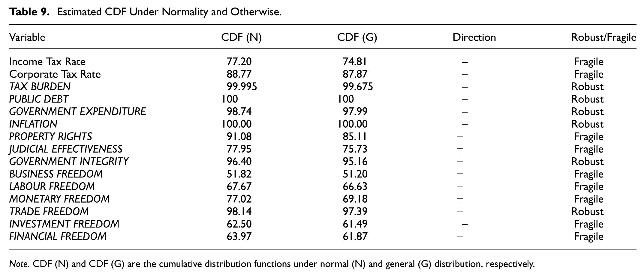
Note. CDF (N) and CDF (G) are the cumulative distribution functions under normal (N) and general (G) distribution, respectively.

In this paper we are interested primarily in the tax and public debt variables. Out of the three tax variables, the most important is tax burden rather than the personal or corporate income tax rates. Two reasons can be suggested for why this is the case. The first is that the tax burden takes into account all taxes at all levels. The effect of an increase in the income tax rate may be offset by a reduction in consumption taxes or the taxes imposed by state and local authorities. The second reason is that wage and salary earners, particularly those in the middle-income group, tend to bear a heavier tax burden since they have fewer opportunities to adjust or reduce their taxable income compared to high-income individuals or corporations. When the tax burden is borne disproportionately by the middle class (people with high marginal propensity to consume) an increase in the tax burden reduces consumption and consequently the willingness of business firms to expand production capacity.

It has become an undisputed fact of life that wage and salary earners pay proportionately more tax than wealthy individuals who generate income from assets and corporations that pay tax on reported accounting income. This is the case because the tax code favors the wealthy and corporations and because they can use “creative” accounting to reduce taxable income. Wage and salary earners do not have this luxury. Leiserson and Yagan (2021) have shown that when an American earns a dollar of wages, that dollar is taxed immediately at ordinary income tax rates, but when they gain a dollar because their stocks increase in value, that dollar is taxed at a low preferred rate, or never at all. One of their findings is that, in the last few years, the average tax rate of the wealthiest 400 US families was 8.2%, much lower than the rate applicable to wage and salary earners.

Other robust variables deserve a brief comment. The finding that government expenditure as a percentage GDP has a negative effect on growth should not be taken at face value. It is not only the quantity that matters, but also the quality of government spending. Common sense tells us that spending on health, education and infrastructure should be conducive to growth, unlike expenditure on the military and spy agencies. These days, governments are more inclined to spend on the military and spy agencies than on health, education and the infrastructure, which may explain the negative relationship between government expenditure and growth. The negative effect of inflation on growth can be explained in terms of any of the cause-effect relations described earlier. The effect is negative because both of these indicators are measured as indices ranging between 0 and 100, which means that a higher number implies more integrity and more freedom. However, it is not clear why trade freedom is more important than any other freedom as envisaged by the Heritage Foundation.

Conclusion

This study examines the effect of taxes and public debt on economic growth. By using a set of cross-sectional data covering 177 countries, we found strong evidence to support the hypotheses that both taxes and public debt retard economic growth. Several statistical and econometric tests were employed to detect the effect of taxes and public debt on growth. These include rank correlation, the classification of observations by high and low percentiles, quantile regression, Leamer’s EBA criterion for robustness, and robustness based on the cumulative distribution function as suggested by Sala-i-Martin (1997).

The five tests and procedures were unanimous in supporting the hypothesis that public debt has a negative impact on growth. The evidence for a negative effect of the tax burden on growth is almost unanimous, except for the Leamer (1985) test, which is very difficult to pass anyway. The negative effect of the personal tax rate is supported by quantile regression and the classification of observations by high and low percentiles. However, no test or procedure supports the hypothesis that reducing the corporate tax rate boosts growth. This is because the corporate sector does not pay its fair share of taxes and indulges in practices that reduce taxable income. The belief that reducing the corporate tax rate is conducive to growth rests on the proposition that when companies have more cash as a result of tax reduction, they invest it in capital accumulation. In reality, they do not, and most of the surplus cash is stashed, used to finance stock buy-backs, or distributed as dividends and bonuses. It is wage and salary earners who bear the brunt of the tax burden, and since these people have high marginal propensities to consume, changes in the personal income tax rate are consequential for aggregate demand.

The implications of these findings are far-reaching. For instance, the findings suggest that alleviating the tax burden on wage and salary earners—who have a high marginal propensity to consume—can enhance aggregate demand and, consequently, stimulate economic growth. Similarly, excessive or persistent reliance on debt financing can undermine growth by crowding out private investment and increasing fiscal vulnerability. Therefore, a sustainable fiscal policy should balance revenue generation with expenditure efficiency, focusing on progressive and growth-oriented tax reforms, prudent debt management, and investment in productivity-enhancing sectors such as health, education, and infrastructure.

Nevertheless, several limitations should be acknowledged. First, the use of cross-sectional data restricts the analysis to a static perspective, preventing the capture of dynamic and causal relationships among fiscal variables and growth over time. In addition, variations in institutional quality, governance structures, and fiscal transparency across countries may influence the magnitude of the observed effects but are not fully addressed within the present framework. Future research could extend this analysis by employing panel or time-series data to capture temporal and causal dynamics, integrating institutional and structural indicators, and exploring non-linear or asymmetric effects of taxation and debt across different income groups, regions, and stages of development. Furthermore, the study highlights that taxes and public debt are not independent fiscal tools, but are intrinsically linked as alternative mechanisms for deficit financing. Future research should model them jointly rather than in isolation.

Footnotes

Acknowledgements

The authors gratefully acknowledge the late Professor Imad A. Moosa for his invaluable contribution to the conception and development of this manuscript. His insight and dedication are deeply appreciated.

We are grateful to the editor and three anonymous referees for useful comments.

ORCID iDs

Ebrahim Merza

Ibrahim N. Khatatbeh

Funding

The authors received no financial support for the research, authorship, and/or publication of this article.

Declaration of Conflicting Interests

The authors declared no potential conflicts of interest with respect to the research, authorship, and/or publication of this article.

Data Availability Statement

“The datasets generated during and/or analysed during the current study are available from the corresponding author on reasonable request.”

References

Aaron

H. J.

Gale

W. G.

Orszag

P. R.

(2004). Meeting the revenue challenge. In Rivlin

A. M.

Sawhill

I. V.

(Eds.), Restoring fiscal sanity (pp. 83–95). Brookings Institution Press.

Abu Alfoul

M. N.

Bazhair

A. H.

Khatatbeh

I. N.

Arian

A. G.

Abu Al-Foul

M. N

. (2024a). The effect of education on economic growth in Sub-Saharan African countries: Do institutions matter? Economies, 12(11), 300.

Abu Alfoul

M. N.

Khatatbeh

I. N.

Bazhair

A. H

. (2024b). The effect of ICT usage on economic growth in the MENA Region: Does the level of education matter? Economies, 12(10), 267.

Alinaghi

Reed

W. R.

(2021). Taxes and economic growth in OECD Countries: A meta-analysis. Public Finance Review, 49, 3–40.

Allard

G. J.

Lindert

P. H.

(2006). Euro-productivity and euro-job since the 1960s: Which institutions really mattered (Working Paper No. 12460). National Bureau of Economic Research.

Auerbach

A. J.

(2002). The Bush tax cut and national saving. National Tax Journal, 55, 387–407.

Bernanke

B. S.

(2010, April 27). Achieving fiscal sustainability, speech before the national commission on fiscal responsibility and reform. http://www.federalreserve.gov/newsevents/speech/bernanke20100427a.htm

Bruno

(1993). Inflation and growth in an integrated approach (Working Paper No. 4422). National Bureau of Economic Research.

Bruno

Easterly

(1996). Inflation and growth: In search of a stable relationship. Federal Reserve Bank of St Louis Economic Review, 78, 139–146.

10.

Calderón

Fuentes

J. R.

(2013). Government debt and economic growth (IDB Working Paper No. IDB-WP-424). Inter-American Development Bank.

11.

CBO. (2001, August). The budget and economic outlook: Update. Ftp://ftp.cbo.gov/30xx/doc3019/EntireReport.pdf

12.

CBO. (2008, January). Options for responding to short-term economic weakness. https://www.cbo.gov/publication/41660?utm_source=chatgpt.com

13.

CBO. (2010, July 27). Federal debt and the risk of a fiscal crisis. Economic and Budget Issues in Brief.

14.

Cecchetti

S. G.

Mohanty

M. S.

Zampolli

(2010, March 26). The future of public debt: Prospects and implications. BIS Working Paper No. 300. Bank for International Settlements (BIS).

15.

Chicago Booth. (2012, June 26). Laffer curve. https://kentclarkcenter.org/surveys/laffer-curve/

16.

Cloyne

Dimsdale

Postel-Vinay

(2018). Taxes and growth: New narrative evidence from Interwar Britain. NBER Working Paper No. 24659. National Bureau of Economic Research (NBER).

17.

de Rugy

Salmon

. (2020, April 15). Debt and growth: A decade of studies. Mercatus Center, George Mason University. Policy Brief.

18.

Durante

(2021, May 21). Reviewing recent evidence of the effect of taxes on economic growth. Tax Foundation.

19.

Elmendorf

D. W.

Reifschneider

D. L.

(2002). Short-run effects of fiscal policy with forward-looking financial markets. National Tax Journal, 55, 357–386.

20.

Feldstein

(1996). The costs and benefits of going from low inflation to price stability. NBER Working Paper No. 5469. The National Bureau of Economic Research (NBER).

21.

Friedman

(2002). No light at the end of the tunnel. http://www.newamerica.net/publications/articles/2002/no_light_at_the_end_of_the_tunnel

22.

Gale

W. G.

Potter

S. R.

(2002, March). An economic evaluation of the economic growth and tax relief reconcilliation act of 2001. National Tax Journal, 55(1), 133–186.

23.

Gale

W. G.

Samwick

A. A.

(2014, September). Effects of income tax changes on economic growth. Economic Studies at Brookings.

24.

Gechert

Heimberger

(2022). Do corporate tax cuts boost economic growth? European Economic Review, 147, 104157.

25.

Gilbert

C. L.

(1986). Professor Hendry’s econometric methodology. Oxford Bulletin of Economics and Statistics, 48, 283–307.

26.

Gravelle

J. G.

Hungerford

T. L.

Labonte

(2009, November 10). Economic stimulus: Issues and policies. Congressional Research Service.

27.

Gunter

Riera-Crichton

Vegh

Vuletin

(2019). Non-linear effects of tax changes on output: The role of the initial level of taxation. NBER Working Paper No. 26570. The National Bureau of Economic Research (NBER).

28.

Heimberger

(2021). Do higher public debt levels reduce economic growth? (Working Paper 211). Vienna Institute for International Economic Studies.

29.

Hoang

L. K.

Cao

B. T.

K. M.

Nguyen

D. T. T.

(2021). Taxation and economic growth: A regression: Analysis based on a new classification. Economic Horizons, 23, 215–229.

30.

Hope

Limberg

(2022). The economic consequences of major tax cuts for the rich. Socio-Economic Review, 20(2), 539–559.

31.

Husak

(2021, June). The relationship between taxation and U.S. economic growth. Washington Center for Equitable Growth.

32.

Jaimovich

Rebelo

(2017). Nonlinear effects of taxation on growth. Journal of Political Economy, 125, 265–291.

33.

Johnson

Papageorgiou

(2020). What remains of cross-country convergence? Journal of Economic Literature, 58, 129–175.

34.

Joint Committee on Taxation. (2005, March). Macroeconomic analysis of various proposals to provide $500 billion in tax relief. JCX-4-05. https://www.jct.gov/getattachment/ab2809ab-57a5-4273-a58f-5375920fc8bb/x-4-05-1611.pdf

35.

Jones

Manuelli

(1993). Growth and the effects of inflation. NBER Working Paper No. 4523. The National Bureau of Economic Research (NBER).

36.

Khatatbeh

I. N.

(2019). The macroeconomic consequences of financialisation [Doctoral dissertation, RMIT University]. Melbourne, Australia.

37.

Khatatbeh

I. N.

Moosa

I. A.

(2022). Financialization and income inequality: An extreme bounds analysis. The Journal of International Trade & Economic Development, 31(5), 692–707.

38.

Kogan

(2003, March 3). Will tax cuts ultimately pay for themselves? Center on Budget and Policy Priorities.

39.

Krugman

(2010, March 12). Debt and transfiguration. New York Times.

40.

Leamer

(1983). Let’s take the con out of econometrics. American Economic Review, 73, 31–43.

41.

Leamer

(1985). Sensitivity analysis would help. American Economic Review, 75, 308–313.

42.

Leiserson

Yagan

(2021, September 23). What is the average federal individual income tax rate on the wealthiest Americans? The White House Blog.

43.

Ljungqvist

Smolyansky

(2018). To cut or not to cut? On the impact of corporate taxes on employment and income. NBER Working Paper No. 20753. The National Bureau of Economic Research (NBER).

44.

Mazerov

(2010, September 14). Cutting state corporate income taxes is unlikely to create many jobs. Centre on Budget and Policy Priorities.

45.

McBride

(2012). What is the evidence on taxes and growth? Tax Foundation Special Report, 207, 1–10.

46.

Mertens

Montiel Olea

J. L.

(2018). Marginal tax rates and income: New time series evidence. Quarterly Journal of Economics, 133, 1803–1884.

47.

Milasia

Waldmann

R. J.

(2018). Top marginal taxation and economic growth. Applied Economics, 50, 2156–2170.

48.

Miller

Kim

A. B.

Roberts

J. M.

(2019). Index of economic freedom. The Heritage Foundation.

49.

Miller

Kim

A. B.

Roberts

J. M.

Tyrrell

(2022). 2022 index of economic freedom. The Heritage Foundation.

50.

Moosa

I. A.

(2014). Quantitative easing as a highway to hyperinflation. World Scientific.

51.

Nguyen

A. D. M.

Onnis

Rossi

(2021). The macroeconomic effects of income and consumption tax changes. American Economic Journal: Economic Policy, 13, 439–466.

52.

Pindyck

Solimano

(1993). Economic instability and aggregate investment. NBER Working Paper No. 4380. The National Bureau of Economic Research (NBER).

53.

Reid

B. M.

(2010, June 21). The three biggest myths about tax cuts and the budget deficit. Heritage Foundation.

54.

Reinhart

C. M.

(2010, February 9). Testimony before the senate budget committee. http://www.scribd.com/doc/58554993/Reinhart-Senate-Testimony-February-9-2010

55.

Reinhart

C. M.

Rogoff

(2009). This time is different: Eight centuries of financial folly. Princeton University Press.

56.

Reinhart

C. M.

Rogoff

(2010). Growth in a time of debt. American Economic Review, 100, 573–578.

57.

Ruffing

Horney

J. R.

(2010, June 28). Critics still wrong on what’s driving deficits in coming years: Economic downturn, financial rescues, and bush era policies drive the numbers. Center on Budget and Policy Priorities.

58.

Sala-i-Martin

(1997). I just ran two million regressions. American Economic Review, 87, 178–183.

59.

Salmon

(2021). The impact of public debt on economic growth. Cato Journal, 41, 487–509.

60.

San

C. K.

Chin

(2023). Impact of public debt on economic growth: A quantile regression approach. South Asian Journal of Macroeconomics and Public Finance, 12, 250–278.

61.

The Economist. (2010, June 26). Repent at leisure (Special Report on Debt). https://www.economist.com/special-report/2010/06/26/repent-at-leisure

62.

Young

Holsteen

(2017). Model uncertainty and robustness: A computational framework for multimodel analysis. Sociological Methods and Research, 46, 3–40.

63.

Zidar

(2019). Tax cuts for whom? Heterogenous effects of income tax changes on growth and employment. Journal of Political Economy, 127, 1437–1472.

The Effect of Tax and Public Debt on Economic Growth: Worldwide Cross-Sectional Evidence

Abstract

Plain Language Summary

Keywords

Introduction

Literature Review: The Effect of Taxes on Economic Growth

Literature Review: The Effect of Public Debt on Growth

Model Specification and the Choice of Explanatory Variables

Estimation Methodology

Data and Preliminary Results

Quantile Regression Results

EBA Results

Conclusion

Footnotes

Acknowledgements

ORCID iDs

Funding

Declaration of Conflicting Interests

Data Availability Statement

References