Sage Journals: Discover world-class research

Abstract

This paper analyzes the October 20, 2019, Bolivian general elections, which led to Evo Morales’ resignation amid widespread fraud allegations. It introduces a theoretical framework to detect irregularities and employs a matching technique to quantify their impact on the election outcome. The study focuses on the vote margin between Morales’ party, Movement Toward Socialism (MAS), and the Citizens Community (CC) party, identifying potential interventions that may have influenced the results. By treating these interventions as treatments applied to specific tally sheets, the study uses matching techniques to compare treated tallies with control tallies from similar geographic and voting patterns. The results suggest that several interventions significantly affected the outcome. Significant deviations were observed in the final tally sheets processed by the electoral authority, many from rural areas expected to favor MAS. However, the margin for MAS in this batch was unusually high compared to similar precincts, localities, or municipalities. Despite a margin exceeding 40% in favor of MAS, our analysis indicates that a much lower margin would have been typical, suggesting atypical voting patterns in these areas. Contrary to popular belief, the most notable trend changes occurred in urban areas by the end of the process.

JEL Classification: C21, C25, D72.

Keywords

Bolivia elections matching fraud

Introduction

On October 25, 2019, Evo Morales, representing the Movement Toward Socialism (Movimiento al Socialismo, MAS), was declared the winner of the Bolivian presidential election with 47.08% of the valid votes, narrowly surpassing the 10% lead required to avoid a runoff. His main opponent, Carlos Mesa, of the Citizens Community (Comunidad Ciudadana, CC), received 36.51%, resulting in Morales’ victory without a second round—despite polls indicating he would likely have lost in a runoff.

However, the results were widely contested by opposition parties, civic groups, and international observers, citing concerns over widespread electoral fraud. Allegations included Morales’ disregard for the 2016 referendum prohibiting his re-election, misuse of public resources, and undue control over state powers such as the electoral authority and media, as noted by the European Union’s Electoral Expert Mission (2019). A major point of controversy arose when the Preliminary Election Results Transmission System (Transmisión de Resultados Electorales Preliminares, TREP) was abruptly suspended for nearly 24 hr. When TREP resumed, the margin in Morales’ favor had unexpectedly increased beyond the crucial 10% threshold, sharply contrasting with earlier results and independent exit polls.

Following public protests, the Organization of American States (OAS, 2019) investigated the election and reported significant discrepancies that cast doubt on its legitimacy, suggesting Morales may not have achieved the margin needed to avoid a runoff. The OAS recommended new elections under a reformed electoral body. Amid growing domestic and international pressure, Morales resigned and sought asylum, plunging Bolivia into political instability. The 2019 election has since become a key case study in the analysis of electoral irregularities and fraud detection.

Detecting electoral irregularities is essential to ensuring democratic legitimacy. Numerous studies have examined electoral fraud, focusing on vote manipulation to benefit incumbents or favored candidates. Skovoroda and Lankina (2017) analyzed inflated turnout and vote redistribution in Russia’s 2011 election using last-digit tests and regression analysis. Beber and Scacco (2012) identified manipulation in fabricated vote counts across Sweden, Senegal, and Nigeria, highlighting systematic human biases. Benford’s Law, commonly used in fraud detection, was applied by Klimek et al. (2018) to Turkey’s constitutional referendum to uncover ballot-stuffing, though Deckert et al. (2011) warned against using it in isolation. Extensions include Mumic and Filzmoser’s (2021) multivariate tests, and alternative methods like integer percentage analysis and co-occurrence heat maps proposed by Lacasa and Fernández-Gracia (2019).

Regression analysis is also a key tool. Enikolopov et al. (2013) used field experiments and instrumental variables in Russia’s 2011 election to show a significant vote drop for incumbents in stations with independent observers. Hausmann and Rigobon (2011) applied similar methods in Venezuela’s 2004 referendum to evaluate electronic fraud. Golden et al. (2015) studied biometric identification machines in African elections, finding higher fraud rates where machines failed.

Christensen and Schultz (2014) proposed a method to detect election fraud before criminal prosecution is possible, focusing on two voter subsets vulnerable to manipulation. They found no evidence of widespread fraud, except for a single known case. In contrast, George (2014) introduced a new socioeconomic parameter to assess fraud in Georgian elections from 1992 to 2012, examining ethnic minority voting, high turnout, and support for the ruling party. Using statistical methods and OLS regression, he analyzed factors such as urban density and minority status, concluding the elections were systematically fraudulent.

Recent studies also incorporate machine learning and simulations. Zhang et al. (2019) used synthetic data and random forest models to predict fraud in Argentina, while Cantú and Saiegh (2011) developed a detection prototype based on Bayesian classifiers. Castañeda and Ibarra (2010) simulated agent behavior in Mexican elections and ruled out large-scale fraud using the Kolmogorov-Smirnov test.

Hicken and Mebane (2015) reviewed forensic methods, including digit distribution analysis and geographic clustering. Eggers et al. (2021) applied these tools to the U.S. elections and found no significant anomalies.

Several studies have assessed the 2019 Bolivian elections and the associated fraud allegations. The Organization of American States (OAS, 2019) identified multiple irregularities, including the suspension of the Preliminary Electoral Results Transmission System (TREP), discrepancies between preliminary and final counts, flaws in the transmission system, the use of a hidden network, and evidence of manipulation—all of which cast doubt on the legitimacy of Evo Morales’ victory. The Comisión Técnica Jurídica (2019) further analyzed arithmetic errors and voter identification issues, confirming irregularities across multiple levels.

Villegas (2019) reported inconsistencies between tally sheets and vote transfers favoring MAS, while Baspineiro and Durán (2019) applied Benford’s Law to the 16% of votes processed after the TREP shutdown and found statistical anomalies. Long et al. (2019) disputed these claims, arguing that pre- and post-shutdown vote trends were consistent and attributing fraud allegations to politicization. Similarly, Williams and Curiel (2020) projected a 10.5% margin for MAS and found no significant discrepancies across the two periods.

Newman (2020) challenged this view using Kolmogorov-Smirnov tests and Oaxaca decompositions, finding a discontinuity in the final 5% of votes. Rosnick (2020) questioned Newman’s methodology, proposing alternative data splits that showed no significant differences. Del Castillo et al. (2019) applied regression discontinuity and probit models, highlighting a rising error frequency as the count progressed, which supported fraud concerns. Idrobo et al. (2022) reexamined these patterns and attributed them to data exclusion. Escobari and Hoover (2024) used minute-by-minute data and difference-in-differences estimates to show that late-arriving votes had a significant effect, with just 2.51% of valid votes enough to change the result.

This paper quantitatively examines the alleged irregularities in the 2019 Bolivian elections and makes three main contributions. First, it develops a simple theoretical model that identifies “efficient” ways to alter election outcomes and the patterns such interventions would generate. Second, it shows that relatively small changes can significantly affect results. Third, it introduces a novel approach for evaluating potential irregularities using matching techniques.

The paper is organized as follows: Section “A simple model on how to conduct electoral fraud” presents the theoretical framework on electoral fraud strategies. Section “The data” describes the data and collection methods. Section “The empirical strategy” outlines the empirical approach. Section “The evidence” analyzes evidence of potential manipulation, voting patterns, and anomalies. Section “Concluding remarks” concludes with a summary of the findings and their implications.

A Simple Model on How to Conduct Electoral Fraud

Imagine you need to manipulate election results to ensure a vote margin over the runner-up exceeds 10% and avoid a runoff.

Define:

M: Vote count for your party,

C: Vote count for the second candidate,

O: Vote count for other candidates,

V: Total valid votes (V = M + C + O)

B: Total invalid votes (blank and null).

The margin between the first and second candidates is:

δ = \frac{M - C}{V} = \frac{M - C}{M + C + O} .

(1)

We introduce operators $d^{+} J and d^{-} K,$ where the first denotes artificially increasing votes for candidate J and the second denotes decreasing votes for candidate K. To increase the margin in (1), we can either increase M or decrease C.

To evaluate each strategy, we totally differentiate (1) considering our definitions of $d^{+} J and d^{-} K,$ yielding:

d δ = \frac{2 C + O}{V^{2}} d^{+} M + \frac{2 M + O}{V^{2}} d^{-} C + \frac{M - C}{V^{2}} d^{-} O .

(2)

Despite its simplicity, expression (2) helps answer key questions: What is the effect on $δ$ when employing different fraud or manipulation strategies? Can we rank these strategies by their effectiveness in increasing $δ$ ?

We term the first strategy “Houdini.” This involves altering the vote count for a candidate by adding or removing votes without affecting other candidates’ tallies. Mathematically, within (1), this means modifying M, C, or O, which in turn affects V (valid votes). To keep the overall vote count unchanged, the Houdini strategy requires that any vote added or removed is offset by an adjustment in blank or invalid votes.

Denote the impact of a Houdini strategy on candidate J as H_J. A Houdini strategy that increases our candidate’s vote count is formulated as:

H_{M} = \frac{d δ}{d^{+} M} = \frac{2 C + O}{V^{2}} > 0 .

(3)

Houdini strategies aimed at decreasing the vote counts of our primary competitor C or another candidate O are formulated as:

H_{C} = \frac{d δ}{d^{-} C} = \frac{2 M + O}{V^{2}} > 0,

(4)

H_{O} = \frac{d δ}{d^{-} O} = \frac{M - C}{V^{2}} > 0, if M > C .

(5)

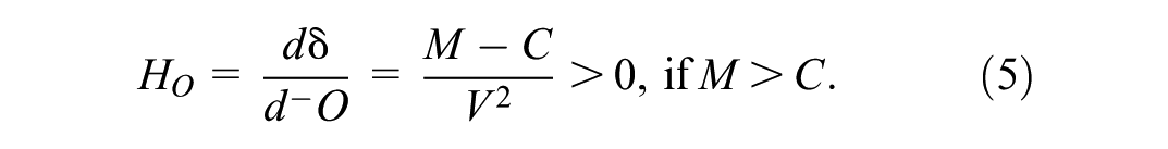
Equations (3) and (4) show that the lead of the first-place candidate over the second increases if the former gains votes or the latter loses them. Equation (5), in contrast, suggests that reducing the vote count for a third candidate (O) benefits only the leader. This is because such a reduction does not change the absolute difference between M and C (the numerator in (1)) but lowers the total valid votes V (the denominator), thereby inflating the percentage margin. While C might have preferred O’s absence before voting—as it could have consolidated the opposition—after voting, reducing O’s count benefits only M and harms C.

The second strategy, termed the “Mutant,” reallocates votes from the closest competitor, candidate C, to the third candidate, O. This maintains the total number of valid votes and the overall vote count. The impact of the Mutant strategy, denoted as U, is:

{U = \frac{d δ}{d^{+} O} |}_{d^{+} O = d^{-} C} = \frac{1}{V} > 0 .

(6)

To achieve this, any increase in votes for candidate O must be offset by an equivalent decrease in votes for candidate C, as stated in (2).

The third strategy, the “Chameleon,” transforms a vote from an opposition candidate into a vote for our candidacy. There are two variants: transferring a vote from the second-place candidate, C, to our candidate, M, and transferring a vote from the third-place candidate to M. The Chameleon strategy applied to candidate J is denoted as A_J. The mathematical representation is:

A_{C} = {\frac{d δ}{d^{+} M} |}_{d^{+} M = d^{-} C} = \frac{2}{V} > 0,

(7)

A_{O} = {\frac{d δ}{d^{+} M} |}_{d^{+} M = d^{-} O} = \frac{1}{V} > 0 .

(8)

After deriving the effects of these strategies, we can rank them by comparing the outcomes from expressions (3) through (8):

\begin{matrix} A_{C} > H_{C} > U = A_{O} > H_{M} > H_{O}, if 3 C + O > M \\ A_{C} > H_{C} > U = A_{O} > H_{O} > H_{M}, if 3 C + O < M \end{matrix} .

(9)

The ranking in (9) reveals several insights: First, employing a Chameleon strategy on candidate C is the most effective. This approach subtracts a vote from our nearest rival and adds it to our tally, without altering the total number of valid votes (denominator in (1)), which is ideal. Next is the Houdini strategy applied to C. It is more detrimental to C to erase their votes than to fabricate votes for our candidate. The Mutant strategy has an equivalent effect as a Chameleon strategy applied to O, as both keep the total valid votes constant, and the numerator changes similarly. The only ambiguous relationships occur between a standard Houdini (H_M) and a Houdini applied to O (H_O). If M has a significant lead over C, it is more advantageous to eliminate votes for O (reducing the denominator in (1)) than to create additional votes for oneself (which also increases the denominator). However, if the margin over the runner-up is not substantial, it is preferable to generate votes for oneself.

To elaborate, change the scenario: Now, our candidate (M) is in second place and aims to close the gap with the first-place candidate (C). When M < C, the following equation applies:

A_{C} > H_{M} > U = A_{O} > H_{C} > H_{O} .

(10)

In this context, Houdini strategies become clear. If M, the second-place candidate, intends to commit fraud, the optimal choice is to generate additional votes for themselves, rather than removing votes from C (first) or O (third). Executing a Houdini on the third-place candidate is ineffective as it inadvertently increases the lead of the first-place candidate over the second. The second-place candidate benefits more from an increase in votes for the third-party candidate than a decrease.

When M is leading and orchestrating fraud, the most effective strategies are a Chameleon or a Houdini targeting the second-place candidate. If these are not feasible, the next best options are a Mutant strategy (shifting votes from the second to the third candidate) or a Chameleon aimed at the third candidate. If the runner-up is close behind, it is more effective for M to apply a Houdini to themselves than to the third candidate. Thus, when M leads and does not use a Mutant strategy, O’s vote count should decrease. If M relies heavily on self-Houdinis and wants to avoid inconsistencies in total votes cast, invalid votes should be reduced. Conversely, a second-place candidate considering fraud should avoid Houdinis on the third candidate, as this would only widen the gap with the frontrunner.

To illustrate, consider the “Base” scenario in Table 1. If current trends continue, the margin between M (the leading candidate) and C (the runner-up) would be close to 10%, potentially requiring a runoff. To avoid this, the objective is to widen the margin by 0.5%, reaching 10.5%. In an electorate of over 6.3 million, a Chameleon strategy targeting the second-place candidate can achieve this shift with just 15,000 votes—about 75 tally sheets, or 0.24% of total votes cast. Less efficient strategies require larger adjustments. For example, using only a Houdini strategy on the third-party candidate would involve altering 286,000 votes. These figures show that changing the margin between the top two candidates using these methods is feasible.

Table 1.

How to Increase Your Vote by 0.5%?

	Base	A_C	H_C	U	A_O	H_M	H_O
C	2,200	2,185	2173	2,170	2,200	2,200	2,200
M	2,800	2,815	2800	2,800	2,830	2,834	2,800
O	1,000	1,000	1000	1,030	970	1,000	714
V	6,000	6,000	5973	6,000	6,000	6,034	5,714
B	320	320	347	320	320	286	606
Total	6,320	6,320	6,320	6,320	6,320	6,320	6,320
δ	10%	10.5%	10.5%	10.5%	10.5%	10.5%	10.5%
Δ	0	15	27	30	30	34	286

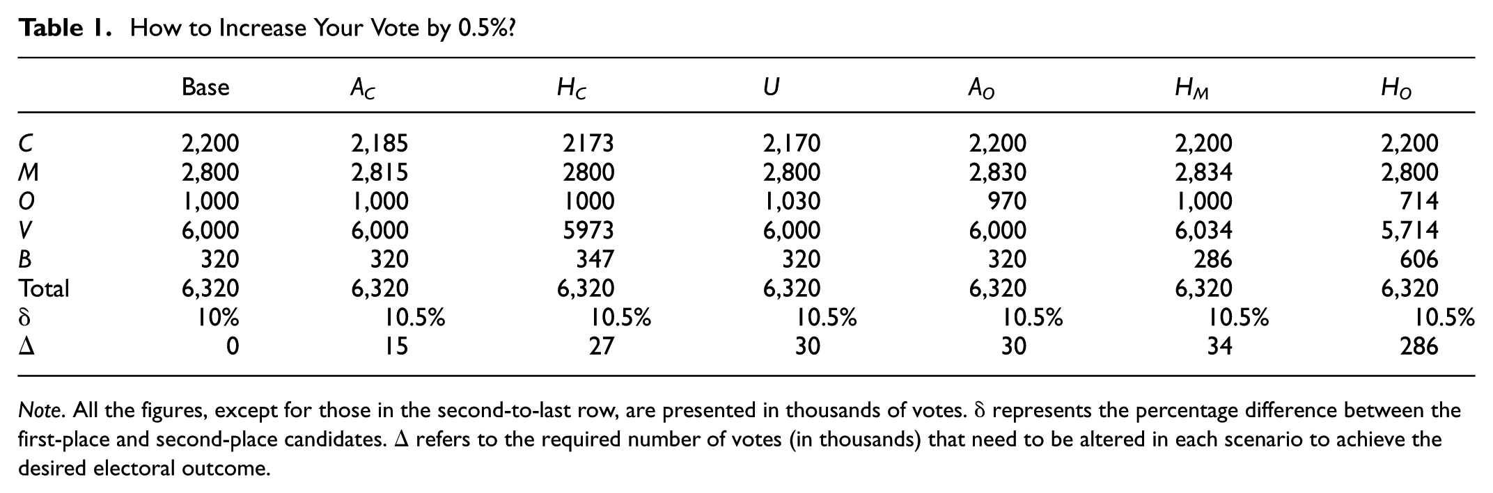
Note. All the figures, except for those in the second-to-last row, are presented in thousands of votes. δ represents the percentage difference between the first-place and second-place candidates. Δ refers to the required number of votes (in thousands) that need to be altered in each scenario to achieve the desired electoral outcome.

The Data

This paper analyzes voting patterns recorded in the TREP and the official counts. In the TREP, results are tabulated from photographs of tally sheets submitted immediately after voting. These records are later validated during the computation stage. A well-functioning TREP process should result in few corrections, so—barring specific justifications—preliminary TREP results and final counts should not differ systematically.

Once the electoral authority receives the tally sheets and begins the official count, TREP data can be compared with the final records. This comparison is used in several studies to detect potential anomalies. Despite multiple interruptions, both the TREP and official tally websites published Excel files with results by tally sheet and allowed users to query individual tallies using a voter’s identity card number or the polling station and tally code. This access triggered widespread social media scrutiny, revealing apparent inconsistencies.

Distinguishing between legitimate corrections and possible manipulation is difficult, as many changes may reflect transcription, transmission, or counting errors. Discrepancies between TREP reports, scanned tally sheets, and final results were sometimes corrected in later updates.

In this study, we analyzed two TREP files (TREP0 and TREP1) and two official count files (COMP0 and COMP1), corresponding to versions released by the electoral management body at different stages: TREP0 was published on October 20, 2019, at 19:40:57, and TREP1 on October 25 at 6:49:40. COMP0 was released on October 21 at 7:49:51, and COMP1— the final version—on October 25 at 17:03:30. Table 2 summarizes key characteristics of these files. For example, TREP0 included 28,975 tally sheets, accounting for over 5.4 million votes, approximately 84% of the final total in COMP1. At that point, the vote margin between MAS and CC was 7.87%.

Table 2.

The TREP and the Final Count.

	TREP0	TREP1	COMP0	COMP1
Tally sheets	28,975	33,044	6,535	34,555
Registered voters	6,137,228	7,016,384	1,407,303	7,315,364
Votes cast	5,415,786	6,194,344	1,250,227	6,460,515
Valid votes	5,152,979	5,885,785	1,193,252	6,137,671
CC	1,950,000	2,162,311	586,070	2,240,920
MAS	2,355,644	2,757,673	418,079	2,889,359
Blank	74,910	89,660	13,925	93,507
Null	187,897	218,899	43,050	229,337
Discrepancies	1,385	1,766	127	950
D0	7.87%	10.12%	−14.08%	10.57%
D1	7.51%	9.78%	−14.20%	10.35%

Note. Discrepancies: Refers to tally sheets with more votes cast than registered voters, incorrect sums of valid votes, or discrepancies in votes compared to the COMP1 file. D0: Represents the percentage difference in votes between MAS and CC as per the respective database. D1: Represents the percentage difference in votes between MAS and CC according to the respective database, excluding tally sheets with discrepancies. Negative values in D0 and D1 indicate that CC is leading over MAS.

The table includes a row indicating the number of tally sheets with discrepancies. These may arise when the total of valid and invalid votes exceeds the number of registered voters, when the sum of votes for all candidates does not match the reported valid votes, or when records in that database differ from the final count (COMP1). A common source of error—regardless of procedural implications—was the mistaken inclusion of blank and invalid votes as valid ones. In TREP1, 5.34% of tally sheets contain at least one such discrepancy, a non-negligible share potentially affecting over 350,000 votes. Remarkably, even in the final count, 950 records (2.75% of total tally sheets) still exhibit arithmetic inconsistencies.

Table 2 shows the vote difference between MAS and CC across the different databases. For example, in the COMP0 count, CC led MAS by 14.08% (row D0). The table also reports the vote margin excluding tally sheets with discrepancies. In all cases, excluding these records improves CC’s standing relative to MAS. This suggests that the discrepancies tend to either harm CC or favor MAS. Notably, while TREP1 shows a margin of over 10% in favor of MAS, this falls to 9.78% once problematic tally sheets are removed—enough to trigger a second round. In addition, 1,511 records (34,555 minus 33,044) were not included in the TREP, making comparisons with the final count impossible for those cases.

In sum, these findings support those of Villegas (2019) and colleagues, who estimated that roughly 5% of tally sheets displayed discrepancies or were modified during the official count.

Table 3 reports the number of discrepancies between preliminary tallies from each TREP session and the final count (COMP1). This conservative estimate likely understates the extent of anomalies, as it records only net changes and consolidates all parties other than MAS and CC under “Others” for simplicity. In TREP1, 1,128 instances involved changes in vote counts for one of the parties or in the number of blank and invalid votes—equivalent to 3.4% of all TREP1 tallies. Following a good-faith approach, records where the sum of candidate votes did not match the reported valid votes were not treated as anomalies.

Table 3.

The TREP and Possible Patterns.

	TREP0	TREP1
Records	872	1,128
A_C	6	8
H_C	39	53
U	7	8
A_O	47	58
H_M	91	122
H_O	191	245

Note. Records: Number of tally sheets in which there are discrepancies in votes between the corresponding TREP and the total count. A_J: Conditions for a Chameleon at J are met; that is, M receives more votes, and J receives fewer votes. H_J: Conditions for a Houdini at J are met; where in the case of M, it means an increase in votes, and for the others, a decrease. U: Condition for a Mutant is met; that is, O’s votes increase, and C’s votes decrease. From this point forward, O is considered the consolidation of other parties that are not M or C.

The table lists cases where conditions for the strategies in Section “A simple model on how to conduct electoral fraud” are met. Comparing TREP1 and COM1 records, there are 122 instances of increased votes for M, 245 of decreased votes for other parties (potential Houdini to O), and 53 of decreased votes for C. Additionally, there are eight instances where C’s votes decrease while O’s votes increase, indicating conditions for Mutants. This suggests these strategies could have been implemented and left traces. Table 3 shows a higher frequency of decreased votes for O than for C, which, although less effective in widening the margin between M and C, is particularly damaging to C as it reduces its margin relative to M.

Could these discrepancies stem from factors other than deliberate fraud—such as human error or incompetence? One recurring issue involves misrecording votes intended for the presidential race as votes for deputies, and vice versa. These mistakes were noted in the minutes but often overlooked during TREP transcription, leading to inconsistencies. Ideally, they should have been corrected during the official count using the original tally sheets. Since turnout for the presidential race typically exceeds that for deputies, proper correction would generally raise presidential vote counts and lower those for deputies.

Discrepancies alone do not explain the increased margin between MAS and CC. MAS’s net gain of 3,661 votes between the initial TREP count and the final tally is minimal and insufficient to account for the 0.5% difference discussed in Section “A simple model on how to conduct electoral fraud.”

Any deliberate falsification of results—regardless of scale—should lead to immediate disqualification and public condemnation of the responsible candidate. Yet while such actions are serious from moral, legal, and ethical standpoints, they may not fully explain the magnitude of the observed differences. Discrepancies between TREP and the official count may reflect both innocent errors and intentional manipulation, often indistinguishably.

Even if individual discrepancies seem minor, their presence does not rule out the possibility that Chameleon, Mutant, or Houdini strategies were used more broadly. These tactics may have left systematic traces not limited to the explicit cases listed in Table 3. If the errors were purely random, no consistent bias would emerge. The fact that irregularities repeatedly favor one candidate suggests a deliberate pattern. The following sections examine specific data patterns in which these strategies may have been applied.

The Empirical Strategy

This study evaluates the likelihood and impact of interventions that may have altered the final election outcome, potentially preventing a runoff between MAS and CC. The analysis focuses on the vote margin between MAS and CC as a percentage of valid votes to assess the impact of these interventions.

Interventions are treated as specific treatments applied to segments of the population. Assuming no systematic differences other than the treatment, the effect can be analyzed as a natural experiment, following the framework of Imbens and Rubin (2015).

The causal estimand of interest when evaluating the effect of a specific treatment, commonly referred to as the Average Treatment Effect on the Treated (ATT), can be defined as:

τ = E [Y_{i} (1) - Y_{i} (0) | D_{i} = 1],

(11)

where $Y_{i} (1)$ corresponds to the outcome of interest (in our case, the difference in votes between MAS and CC) of tally i that is subject to the treatment, $Y_{i} (0)$ is the potential outcome if tally i had it not been treated, and $D_{i} = 1$ represents the specific intervention for which we want to evaluate if there are differences.

The ATT measures the difference between the actual outcome for the treated units and the hypothetical outcome they would have experienced had they not received the treatment. Since the counterfactual outcome is unobservable, an appropriate control group is required for comparison.

The key question is whether the behavior of potentially intervened records (treated group) aligns with non-intervened records (control group). For each treated tally, control tally sheets from similar contexts are identified, expecting comparable voting behaviors in the absence of irregularities.

Similarity is based on voting or residence location. Control groups are identified using data on the department (or country), province, municipality, locality, and voting precinct for each record. Ideally, control tallies from the same polling station and numerically adjacent to the treated tallies are selected. If no exact matches are found, the search extends to all tallies from the same station, locality, municipality, and province, considering the urban or rural condition.

This conservative method focuses on the closest matches to estimate differences between treated and control groups. However, it may not detect precinct-level irregularities, potentially showing no difference despite irregularities.

The Evidence

Sections “A simple model on how to conduct electoral fraud” and “The data” show that electoral outcomes—especially those determined by narrow margins—are highly sensitive to small shifts. A 0.5% change in the vote margin between leading candidates can result from adjustments to just 0.24% of total votes, or roughly 75 polling stations. Discrepancies between TREP data and the final count were found in 5% of cases analyzed, suggesting that modifications to tally sheets could have significantly affected the result.

This section quantifies the potential impact of such irregularities. Given the high stakes at the time, the focus is on the most prominent scenarios. The approach is consistent: we adopt a “benign” explanation as the null hypothesis for each suspected irregularity, and then test whether the data supports it.

Flying Under the Radar (to TREP or Not to TREP)

Could the widening vote margin between MAS and CC be explained by something other than discrepancies between TREP records and the official count? Yes—one key overlooked factor is TREP’s incomplete coverage. As noted in Section “The data” and shown in Table 2, 1,511 tally sheets included in the final count were never captured by TREP.

Do the records omitted from the TREP exhibit similar patterns to those included? If not, the differences may not be fully explained by benign errors like human transcription mistakes. If the comparison is conducted correctly, discrepancies cannot be attributed to differences in other characteristics either.

Table 4 revisits the findings from Table 2, focusing on discrepancies between TREP and the final count (COMP1). A shift in the MAS–CC vote margin is evident between TREP0 and TREP1, but it is far less dramatic than the gap between the TREP-covered records and the 1,511 tallies omitted from TREP (the “NO TREP” column in Table 4). In these overlooked records, the margin widens to nearly 21%—more than double that seen in TREP1—raising a key question: can such a large increase be explained by benign factors?

Table 4.

Unconditional Comparison Between Tallies With and Without TREP.

	TREP0	TREP1	NO TREP	COMP1
Tally sheets	28,975	33,044	1,511	34,555
Registered voters	6,137,228	7,016,384	298,980	7,315,364
Votes cast	5,415,786	6,197,056	263,459	6,460,515
Valid votes	5,152,979	5,889,920	247,751	6,137,671
CC	1,950,000	2,164,605	76,315	2,240,920
MAS	2,355,644	2,761,334	128,025	2,889,359
D0	7.87%	10.13%	20.87%	10.57%

Note. D0: Percentage difference in the vote between the MAS and CC according to the corresponding database.

The most direct explanation is that the NO TREP records represent a different population from the TREP-covered ones. For instance, if TREP1 largely captures urban areas while NO TREP includes mostly rural ones, such discrepancies could arise naturally. A valid comparison, then, requires identifying a population similar to the NO TREP group.

Starting with the 1,511 NO TREP records, I excluded two annulled tallies with no voting data. Of the remaining 1,509, one was dropped due to the absence of suitable matches in the same precinct. For the final 1,508 records, I identified counterparts from the control population at the most granular level available, prioritizing matches from neighboring tallies or within the same precinct. I then compared party vote percentages between these groups to assess whether statistically significant differences emerged.

Table 5 compares voting patterns from records not included in the TREP with similar ones that were, ideally from the same voting location. The analysis controls for whether the area is urban or rural. At the locality level, MAS outperforms its matched counterparts by a statistically significant 1.62% in valid votes. When matching is refined to the neighbor or precinct level, CC receives fewer votes and MAS more, though the difference is smaller and not statistically significant.

Table 5.

Comparison Between TREP and NO TREP.

	NO TREP	Diff 1	Diff 2
Percentage C	29.12	−0.86 (0.31)	−0.27 (0.23)
Percentage M	52.92	0.76 (0.34)	0.22 (0.29)
Percentage O	17.95	0.10 (0.20)	0.05 (0.19)
D0	23.80	1.62 (0.62)	0.49 (0.49)
Percentage B	2.45	0.26 (0.11)	0.21 (0.11)
Percentage N	4.41	0.22 (0.10)	0.15 (0.11)
Turnout	88.27	0.33 (0.14)	0.28 (0.14)

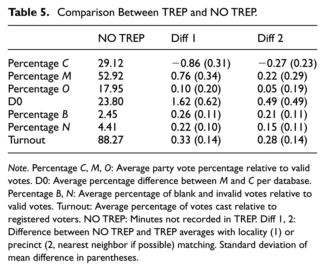
Note. Percentage C, M, O: Average party vote percentage relative to valid votes. D0: Average percentage difference between M and C per database. Percentage B, N: Average percentage of blank and invalid votes relative to valid votes. Turnout: Average percentage of votes cast relative to registered voters. NO TREP: Minutes not recorded in TREP. Diff 1, 2: Difference between NO TREP and TREP averages with locality (1) or precinct (2, nearest neighbor if possible) matching. Standard deviation of mean difference in parentheses.

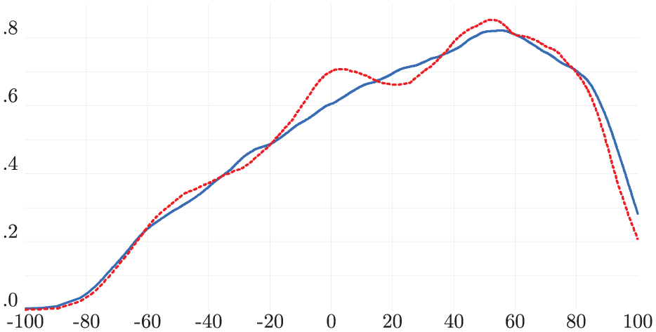
Figure 1 reveals significant heterogeneity within the control group, with multiple modes—one indicating a higher concentration of votes for MAS. This pattern is not mirrored in the NO TREP distribution, where the most pronounced mode shows a difference of at least 80% in favor of MAS. Notably, 10 tally sheets report 100% of votes for MAS, and 125 show margins exceeding 80%. In polling stations where MAS received all the votes, no non-MAS delegates were present—except in one case.

Figure 1.

The behavior of the NO TREP minutes is different.

The control group distribution is more symmetrical and has a less pronounced right tail compared to the NO TREP records.

Applying the 1.62% margin advantage found in Table 5 to the 247,751 valid votes from NO TREP minutes yields a gain of just over 4,000 votes for MAS. However, this increase is not enough to close the 0.57% margin that would have forced a runoff.

Although analyzing discrepancies in the 1,511 NO TREP records might seem unfeasible, a workaround was developed. A group of Bolivian scientists created a now-defunct website (https://www.mivotobolivia.org/) that allowed citizens to upload photos of polling station results. This initiative provided access to presidential vote counts from 1,004 of the 1,511 missing tally sheets, enabling comparison with the final count.

Of these 1,004 records, 454 (over 45%) included annotations in the minutes. Moreover, 991 (nearly 99%) showed at least one discrepancy between the photographic evidence and the official tally. More than 40% had arithmetic errors, and in 12% of cases, the total votes exceeded the number of registered voters.

On average, discrepancies between the photos and the final tally added 1.32 votes for MAS and 0.44 for CC. While some of this variation may reflect the types of errors discussed in Section “The data,” the average margin based on photographic evidence is nearly 1% smaller than in the final count. Of the 1,004 records, 119 contain arithmetic inconsistencies. Although these discrepancies do not dramatically alter vote totals, they show a consistent bias in favor of MAS.

The Blackout

Controversy arose from a TREP data transmission “blackout” (commonly referred to as an apagón in Bolivia and in the election forensics literature) after 84% of votes had been counted, with MAS leading CC by less than 8%. According to the data transmission company, the halt was ordered by the electoral authority—not due to technical issues. When TREP resumed nearly 24 hr later, the margin had widened to over 10%. As reported by the OAS (2019), unplanned servers had been added to the infrastructure during this period, diverting TREP data. These servers were used to transcribe and verify tally sheets, and at least one remained active even after TREP was officially shut down.

Table 6 shows that voting records processed during the blackout behaved differently from those tallied before, significantly impacting the final outcome. While geography or rural votes might explain these discrepancies, it is crucial to evaluate if these differences were expected based on the vote characteristics during the blackout.

Table 6.

Unconditional Comparison Between Tallies Before and After the “blackout”.

	TREP0	TREP1	BLACKOUT	COMP1
Tally sheets	28,975	33,044	4,069	34,555
Registered voters	6,137,228	7,016,384	879,156	7,315,364
Votes cast	5,415,924	6,194,344	778,420	6,460,515
Valid votes	5,153,112	5,885,785	732,673	6,137,671
CC	1,950,074	2,162,311	212,237	2,240,920
MAS	2,355,683	2,757,673	401,990	2,889,359
D0	7.87%	10.11%	25.90%	10.57%

Note. D0: Percentage difference in the vote between the MAS and CC according to the corresponding database.

Table 7 compares records processed during the blackout with those processed earlier. CC received 3.85% to 0.65% fewer votes than expected based on the geography of blackout records, while MAS received 3.05% to 0.63% more. The gap between candidates widened by 6.90% to 1.28% relative to matched controls. Blank and invalid votes also increased during the blackout, though voter turnout remained stable. These comparisons are based on a hierarchical matching process: 2,202 records were matched at the nearest-neighbor level, followed by 1,178 at the precinct level, 90 at the locality level, 568 at the municipal level, 11 at the provincial level, and 18 from outside Bolivia matched at the country level.

Table 7.

Effect of the Blackout.

	BLACKOUT	Diff 1	Diff 2
Percentage C	28.40	−3.85 (0.22)	−0.65 (0.12)
Percentage M	55.31	3.05 (0.20)	0.63 (0.14)
Percentage O	16.29	0.81 (0.10)	0.02 (0.09)
D0	26.92	6.90 (0.41)	1.28 (0.25)
Percentage B	2.26	0.34 (0.07)	0.25 (0.07)
Percentage N	4.38	0.32 (0.05)	0.18 (0.05)
Turnout	88.56	0.15 (0.08)	0.01 (0.07)

Note. Percentage C, M, O: Average of the party’s percentage of votes in relation to valid votes. D0: Average of the percentage difference in the vote between M and C according to the corresponding database. Percentage B, N: Average percentage of blank and invalid votes with respect to valid votes. Turnout: Average percentage of votes cast with respect to those registered. BLACKOUT: Minutes introduced after the blackout. Diff 1, 2: Difference between the average before and after the blackout with matching at the level of locality (1) or precinct (2, reaching to nearest neighbor when possible). Standard deviation of mean difference in parentheses.

Figure 2 shows distinct patterns in data from minutes processed during the blackout versus before it. The blackout period’s distribution is notably asymmetrical, with a mode where the MAS-CC margin is around 53%. This contrasts with the comparison group, which suggests more variability should have been observed.

Figure 2.

The behavior of the BLACKOUT minutes is different.

These findings highlight the improbability of the observed shift in the MAS-CC margin. Applying the 6.90% (and 1.28%) increase in MAS’s margin during the blackout minutes—as detailed in Table 6 and adjusted for local precinct matching—to the 732,673 affected votes results in an excess of about 50,000 (and 9,000) votes. These numbers could potentially alter the final margin of victory, which was only 0.57%.

Arithmetical Errors

Another controversy involves tallying errors within the minutes, such as mismatched valid vote counts and totals exceeding registered voters. The final count still contains 950 such errors. The question is whether these discrepancies follow a pattern, suggesting they might not be simple arithmetic mistakes.

Table 8 shows that minutes with arithmetic inconsistencies have a larger voting margin favoring MAS over CC. However, this does not imply misconduct. As discussed in Section 3, non-fraudulent explanations exist, such as mistakenly counting blank and invalid votes as valid without adjusting party vote totals.

Table 8.

Unconditional Comparison Between Tallies With and Without Arithmetical Errors.

	WITHOUT	WITH	COMP1
Tally sheets	33,605	950	34,555
Registered voters	7,113,575	201,789	7,315,364
Votes cast	6,283,818	176,697	6,460,515
Valid votes	5,970,290	167,381	6,137,671
CC	2,186,222	54,698	2,240,920
MAS	2,804,249	85,110	2,889,359
D0	10.35%	18.17%	10.57%

Note. D0: Percentage difference in the vote between the MAS and CC according to the corresponding database. WITHOUT: Minutes in which all the sums coincided. WITH: Minutes in which there was some arithmetical inconsistency.

Table 9 shows that discrepancies between records with arithmetic errors and their matched counterparts are not substantial. The differences are statistically significant at the locality level but not at the precinct level. Contrary to expectations, CC did not receive a higher vote share, nor did MAS receive less. Applying the 1.94% additional margin for MAS (from Table 8, locality level) to the 167,381 affected votes yields a net gain of just over 3,200 votes—insufficient to significantly alter the overall margin. Still, it is notable that the final count includes these inconsistencies in roughly 3% of the records, including 22 min where votes were allocated to candidates but not recorded as valid, and 7 minutes where MAS votes exceeded the total number of valid votes.

Table 9.

Effect of Arithmetical Errors.

	WITH	Diff 1	Diff 2
Percentage C	32.11	−1.22 (0.42)	−0.20 (0.22)
Percentage M	51.23	0.71 (0.40)	−0.03 (0.27)
Percentage O	16.66	0.51 (0.22)	0.23 (0.21)
D0	19.13	1.94 (0.78)	0.16 (0.44)
Percentage B	2.06	0.44 (0.15)	0.44 (0.15)
Percentage N	3.87	0.13 (0.10)	0.15 (0.11)
Turnout	87.62	−0.54 (0.18)	−0.60 (0.17)

Note. Percentage C, M, O: Average of the party’s percentage of votes in relation to valid votes. D0: Average of the percentage difference in the vote between M and C according to the corresponding database. Percentage B, N: Average percentage of blank and invalid votes with respect to valid votes. Turnout: Average percentage of votes cast with respect to those registered. WITH: Minutes with arithmetical inconsistencies. Diff 1, 2: Difference between the average with and without mathematical errors with matching at the level of locality (1) or precinct (2, reaching to nearest neighbor when possible). Standard deviation of mean difference in parentheses.

Changing Trends

The election results debate frequently focused on “suspicious” shifts in voting trends. NeoTec’s director mentioned that the TREP blackout was due to an advisory from the electoral body about “sudden changes in the trend” between MAS and CC, favoring CC. Conversely, analysts noted these suspicious shifts favored MAS. On election night, Evo Morales expressed confidence in a first-round victory, attributing a “change in trend” to the rural vote.

Table 10 organizes the 34,555 total tally sheets by the order in which they were reported in the official count and divides them into quintiles. Q₁ represents the first 20% of processed records, Q₂ the next 20%, and so on through Q₅, which includes the final 20%. It is worth noting that the number of votes in each quintile is not uniform, as the last two groups correspond to areas with lower population density.

Table 10.

Unconditional Comparison Between Tallies in Different Quantiles.

	Q ₁	Q ₂	Q ₃	Q ₄	Q ₅	COMP1
Tally sheets	6,911	6,911	6,911	6,911	6,911	34,555
Registered voters	1,482,715	1,465,541	1,507,133	1,457,420	1,402,555	7,315,364
Votes cast	1,315,947	1,306,328	1,326,896	1,245,379	1,265,965	6,460,515
Valid votes	1,254,107	1,243,693	1,269,771	1,182,821	1,187,279	6,137,671
CC	605,275	496,186	493,591	400,667	245,201	2,240,920
MAS	450,041	571,257	581,825	556,486	729,750	2,889,359
D0	−12.38%	6.04%	6.95%	13.17%	40.81%	10.57%

Note. D0: Percentage difference in the vote between the MAS and CC according to the corresponding database. Q_j: Minutes corresponding to the percentile (j − 1) × 100 to j × 100 of the distribution of valid votes processed. COMP1: Final count.

The first quintile heavily favored CC, with a lead of over 12%. The second and third quintiles shifted to MAS, each showing a margin of more than 6%. The most dramatic changes occurred in the last two quintiles: MAS’s lead rose to over 13% in the fourth and exceeded 40% in the final. Cumulatively, CC led by 12.38% after the first 20% of tallies. That lead narrowed to 3.21% after 40%, and by the 60% mark, MAS had edged ahead by 0.21%. With 80% processed, MAS’s lead reached 3.31%, and after the final 20%, it reached 10.57%. These shifts underscore the high variability in voting patterns across quintiles.

Plausible, non-malicious explanations may account for the substantial differences across quintiles. Notably, no fraud accusations were raised when CC led by over 12% in the first quintile. These shifts may reflect Bolivia’s demographic and political diversity. If tally sheets are processed sequentially, covering demographically similar populations over extended periods, shifts in voting margins are expected. Over time, such variations should average out, aligning with broader national trends—offering a straightforward explanation for the observed “trend reversals.”

To test for irregularities across voting groups, I treat each quintile as a treatment group and the remaining four as controls. This framework is appropriate when systematic differences between groups make direct comparisons invalid.

For each record in a quintile, I identify the closest match among those in the other four, prioritizing the nearest neighbor or, if unavailable, a record from the same precinct, locality, or municipality. This matching strategy controls for observable differences and helps ensure that the control group’s behavior is not biased by its order in the final count.

Table 11 shows the comparison results for the last 80% of votes, which exhibited the most significant differences and potential voting trend shifts. Votes for CC were expected to be 3.15% higher and votes for MAS 1.83% lower in this category. The margin difference between the last 80% and comparable records processed before is nearly 5%. These results are broadly consistent with Del Castillo et al. (2019).

Table 11.

Time Effect.

	Q ₅	Diff 1	Diff 2
Percentage C	19.72	−2.97 (0.16)	−3.15 (0.15)
Percentage M	62.49	1.65 (0.17)	1.83 (0.16)
Percentage O	17.79	1.32 (0.10)	1.32 (0.09)
D0	42.77	4.62 (0.32)	4.98 (0.29)
Percentage B	2.58	0.63 (0.05)	0.61 (0.05)
Percentage N	4.51	0.40 (0.04)	0.38 (0.04)
Turnout	90.18	−0.41 (0.06)	−0.41 (0.06)

Note. Percentage C, M, O: Average of the party’s percentage of votes in relation to valid votes. D0: Average of the percentage difference in the vote between M and C according to the corresponding database. Percentage B, N: Average percentage of blank and invalid votes with respect to valid votes. Turnout: Average percentage of votes cast with respect to those registered. Q₅: Last 20% of the minutes processed. Dif 1, 2: Difference between the average processed in Q₅ or processed in Q₁- Q₄ with matching at the level of locality (1) or precinct (2, reaching to nearest neighbor when possible). Standard deviation of mean difference in parentheses.

Applying the unexplained 4.98% margin from the last 80% of tally sheets to the 1,187,279 valid votes in that group yields an excess of just over 59,000 votes—surpassing the combined effect of previously discussed factors. This represents just under 1% of the total valid vote. Several precincts in this category were counted only in the final stage, so matching relied on broader levels—locality or municipality—potentially overstating the difference. However, there is also a risk of underestimating irregularities: if systemic issues occurred at the precinct level, the control group may have been similarly affected, masking discrepancies. Of the matches used, 1,383 were at the nearest-neighbor level, 283 at the precinct level, 1,541 at the locality level, 537 at the municipal level, 707 at the provincial level, and 2,456 at the country level (primarily for records from abroad). In addition, 3 min were annulled, and one (from Colombia) had no match.

The effects may intersect. Of the 1,511 records not in the TREP (Section “Flying under the radar (to TREP or not to TREP)”), 26% were processed in the final phase (last 80%), and 35% of records processed during the TREP “blackout” fall into this phase. Examining overlaps among these groups offers a valuable opportunity to identify the origins and characteristics of these anomalies.

The Final Countdown

The 2019 OAS report highlighted possible unexplained shifts in voting trends toward the end of the tally, particularly within the final 5% of records. This issue has been the focus of several studies. Williams and Curiel (2020) found no evidence of irregularities. In contrast, Newman (2020), Molina (2020), and Escobari and Hoover (2024) identified unusual increases in the MAS vote margin in the final 5%, suggesting discrepancies that merit closer examination.

Table 12 shows that for the first 95% of processed ballots, the margin between MAS and CC remained below 9%. Had this trend continued, a second-round vote would have been required. However, the final 5% of votes counted were disproportionately favorable to MAS, with a margin exceeding 45%. This sharp shift played a decisive role in the final outcome.

Table 12.

Unconditional Comparison of the Last 5% of the Tallies.

	FIRST	LAST	COMP1
Tally sheets	32,827	1,728	34,555
Registered voters	6,987,885	327,479	7,315,364
Votes cast	6,172,351	288,164	6,460,515
Valid votes	5,872,076	265,595	6,137,671
CC	2,188,560	52,360	2,240,920
MAS	2,715,512	173,847	2,889,359
D0	8.97%	45.74%	10.57%

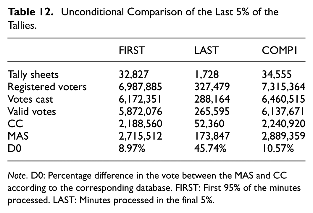
Note. D0: Percentage difference in the vote between the MAS and CC according to the corresponding database. FIRST: First 95% of the minutes processed. LAST: Minutes processed in the final 5%.

Several benign explanations have been proposed for this pattern. Evo Morales claimed that these votes came primarily from rural areas, where his party has historically performed well. Yet the data indicate that rural tallies made up just under 70% of the final 5%—a proportion similar to that of the last three quintiles overall. This weakens the claim that rural dominance alone explains the observed late surge.

Following the approach used in Section “Changing trends,” each record within the final 5% of the count was matched to a counterpart drawn from the first 95%. Matching was prioritized by proximity: first at the nearest-neighbor level, and if unavailable, within the same precinct, locality, or municipality. Among the matches, 578 were at the nearest-neighbor level, 34 at the precinct level, 24 at the locality level, 481 at the municipal level, 336 at the provincial level, and 272 at the country level (primarily for records from abroad). Three minutes were annulled and excluded from analysis.

Table 13 summarizes the results of this analysis. It shows that both CC and the Other Candidates received significantly fewer votes than expected, with MAS absorbing most of the unexplained difference. The unexpected margin reaches nearly 8% when matching at the venue level and close to 9% at the locality level. Applying the average unexplained margin of 7.72% to the 265,595 valid votes in the final 5% of tallies yields an excess of approximately 20,500 votes—enough to account for the narrow margin that avoided a second round.

Table 13.

The Final Countdown.

	LAST	Diff 1	Diff 2
Percentage C	18.13	−2.79 (0.29)	−2.06 (0.27)
Percentage M	67.17	6.10 (0.42)	5.66 (0.41)
Percentage O	14.70	−3.32 (0.29)	−3.59 (0.29)
D0	49.04	8.89 (0.66)	7.72 (0.63)
Percentage B	3.78	−0.46 (0.16)	−0.50 (0.16)
Percentage N	5.28	0.31 (0.09)	0.21 (0.10)
Turnout	87.98	−0.69 (0.13)	−0.75 (0.13)

Note. Percentage C, M, O: Average of the party’s percentage of votes in relation to valid votes. D0: Average of the percentage difference in the vote between M and C according to the corresponding database. Percentage B, N: Average percentage of blank and invalid votes with respect to valid votes. Turnout: Average percentage of votes cast with respect to those registered. LAST: Minutes processed in the final 5%. Diff 1, 2: Difference between the average processed before and after the last 5% of the minutes with matching at the level of locality (1) or precinct (2, reaching to nearest neighbor when possible). Standard deviation of mean difference in parentheses.

Myth Versus Reality

Evo Morales and various analysts have emphasized the critical role of the rural vote in determining the election’s outcome, particularly in the final tally.

Table 14 reveals several notable findings. Contrary to some claims, the majority of votes tallied in the last 20% of the final count were not from rural areas, nor were most of the records processed rural. However, the voting margin for MAS, in both urban and rural settings, significantly exceeded the margins observed in the first 80% of votes counted.

Table 14.

Comparison of Urban and Rural Minutes in the Last 5% of the Vote.

	URBAN	RURAL	COMP1
Tally sheets	3,486	3,352	34,555
Registered voters	772,427	613,788	7,315,364
Votes cast	704,105	549,711	6,460,515
Valid votes	667,140	508,906	6,137,671
CC	179,177	62,387	2,240,920
MAS	357,549	366,616	2,889,359
D0	26.74%	59.78%	10.57%

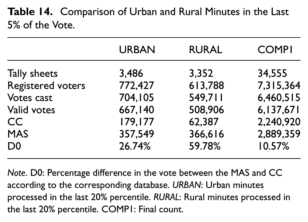
Note. D0: Percentage difference in the vote between the MAS and CC according to the corresponding database. URBAN: Urban minutes processed in the last 20% percentile. RURAL: Rural minutes processed in the last 20% percentile. COMP1: Final count.

Table 15 compares voting outcomes between urban and rural areas in the final 20% of ballots processed. Contrary to expectations, MAS’s margin in rural areas was slightly lower than predicted, while in urban areas it was significantly higher. In the last 5% of records, MAS outperformed expectations by 9.77% in urban areas and 6.83% in rural ones. The unexpected margin in urban areas alone accounts for more than 71,000 votes. These results challenge the narrative that rural votes were primarily responsible for the late shifts in voting trends, suggesting instead that urban areas played a key role in driving the final margin—both in the last 20% and especially within the final 5% of the official count. The magnitude of these differences is sufficient to explain the margin that precluded a runoff.

Table 15.

The Big Differences.

	URBAN	Difference	RURAL	Difference
Percentage C	27.10	−6.64 (0.19)	11.76	0.43 (0.21)
Percentage M	53.31	4.09 (0.17)	72.32	−0.52 (0.26)
Percentage O	19.59	2.54 (0.10)	15.92	0.09 (0.16)
D0	26.22	10.73 (0.35)	60.56	−0.95 (0.45)
Percentage B	1.66	0.61 (0.06)	3.52	0.58 (0.08)
Percentage N	4.10	0.66 (0.04)	4.91	0.09 (0.07)
Turnout	91.18	−0.04 (0.05)	89.48	−0.94 (0.10)

Note. Percentage C, M, O: Average of the party’s percentage of votes in relation to valid votes. D0: Average of the percentage difference in the vote between M and C according to the corresponding database. Percentage B, N: Average percentage of blank and invalid votes with respect to valid votes. Turnout: Average percentage of votes cast with respect to those registered. URBAN: Urban minutes processed in the final 20%. RURAL: Rural minutes processed in the final 20%. Difference: Difference between the average processed before and after the last 20% of the minutes, with matching at the level of precinct (reaching to nearest neighbor when possible). Standard deviation of mean difference in parentheses.

Concluding Remarks

This paper develops a systematic framework to identify post-election irregularities by establishing testable hypotheses for patterns consistent with manipulation. Using matching techniques, it shows how targeted interventions can decisively influence outcomes.

While focused on Bolivia, the findings offer broader lessons. Similar patterns appeared in the 2024 Venezuelan presidential election, where the vote count was halted after 30% of results were reported. The electoral court then declared Nicolás Maduro the winner without releasing polling station records. Opposition groups later posted over 80% of tally sheets online, showing a clear victory for Edmundo González. Both cases illustrate how interruptions and lack of transparency can compromise electoral integrity. They underscore the need for robust international standards in election monitoring.

Statistical analysis, as applied here, is a powerful tool for detecting anomalies and guiding forensic audits. Matching methods can serve as early-warning systems, helping oversight bodies focus resources. In Bolivia, the OAS (2019) conducted forensic evaluations of physical tally sheets to uncover discrepancies. This study shows that statistical analysis can independently identify patterns warranting such scrutiny. It also finds that the most substantial irregularities were concentrated in the final set of processed tallies, particularly in urban areas—contrary to common belief.

The methodology presented here can be applied to other elections, but it requires detailed electoral records. Photographic evidence of tally sheets, when available, adds a valuable layer of verification.

Matching techniques depend on the comparability of treated and control groups, which is more reliable at lower aggregation levels. Their effectiveness also hinges on the availability and quality of control records. Despite these constraints, the framework offers a practical approach for identifying and assessing electoral anomalies in various contexts.

This study contributes to the literature by formalizing strategies of fraud—“Chameleons,”“Mutants,” and “Houdinis”—and showing how even small, systematic interventions can alter results in close elections. It highlights the importance of transparency and institutional safeguards in defending democratic processes. By integrating statistical methods into electoral oversight, practitioners and policymakers can improve detection, enhance credibility, and help protect the integrity of democratic systems.

Footnotes

Appendix

This Appendix presents two conventional empirical exercises conducted to evaluate the presence of irregularities in electoral processes.

Acknowledgements

I would like thank Jorge Abela, Lykke Andersen, Pablo Mendieta, Alejandro Mercado, Jaime Pérez, Ernesto Sheriff, three anonymous referees, and participants of seminars organized by CEDLA, Universidad Católica Boliviana, Universidad Privada de Bolivia, and Universidad Privada de Santa Cruz. I would also like to thank Esteban Calisaya, Flavio Díaz, Marina Dockweiler, Joaquín Morales, Eliana Quiroz, and other individuals who chose to remain anonymous, that provided information necessary for the construction of the data base and conducting the analysis.

Author Note

A version of the paper in Spanish (Chumacero, 2019) was written while the events were unfolding (first draft on October 26, 2019). The usual disclaimer applies.

ORCID iD

Rómulo A. Chumacero

Funding

The author received no financial support for the research, authorship, and/or publication of this article.

Declaration of Conflicting Interests

The author declared no potential conflicts of interest with respect to the research, authorship, and/or publication of this article.

Data Availability Statement

Data sharing not applicable to this article as no datasets were generated or analyzed during the current study.

References

Baspineiro

Durán

(2019). Informe de Observaciones Técnicas al Proceso de Cómputo de Resultados de las Elecciones Presidenciales Octubre 2019. Universidad de San Francisco Xavier.

Beber

Scacco

(2012). What the numbers say: A digit-based test for election fraud. Political Analysis, 20(2), 211–234.

Cantú

Saiegh

(2011). Fraudulent democracy? An analysis of Argentina’s infamous decade using supervised machine learning. Political Analysis, 19(4), 409–433.

Castañeda

Ibarra

(2010). Detección de Fraude con Modelos Basados en Agentes: Las Elecciones Mexicanas de 2006. Perfiles Latinoamericanos, 18(36), 43–69.

Christensen

Schultz

(2014). Identifying election fraud using orphan and low propensity voters. American Politics Research, 42(2), 311–337.

Chumacero

(2019). El Camaleón, el Mutante y Houdini: Resultados de las elecciones en Bolivia. University of Chile.

Comisión Técnica Jurídica. (2019). Análisis de los Resultados Electorales de la Elección Nacional de 20 de Octubre de 2019. Universidad Mayor de San Andrés.

Del Castillo

Morales

Peres

Sheriff

(2019). Análisis Dinámico del Cómputo de Resultados Electorales, Bolivia 2019.

Deckert

Myagkov

Ordeshook

(2011). Benford’s law and the detection of election fraud. Political Analysis, 19(3), 245–268.

10.

Diekmann

(2007) Not the first digit! Using Benford’s law to detect fraudulent scientific data. Journal of Applied Statistics, 34(3), 321–329.

11.

Eggers

Garro

Grimmer

(2021). No evidence for systematic voter fraud: A guide to statistical claims about the 2020 election. Proceedings of the National Academy of Sciences of the United States of America, 118(45), e2103619118.

12.

Enikolopov

Korovkin

Petrova

Sonin

Zakharov

(2013). Field experiment estimate of electoral fraud in Russian parliamentary elections. Proceedings of the National Academy of Sciences of the United States of America, 110(2), 448–452.

13.

Escobari

Hoover

(2024). Late-arriving votes and electoral fraud: A natural experiment and regression discontinuity evidence from Bolivia. World Development, 173, 106407.

14.

European Union. (2019). Election Expert Mission: Bolivia 2019 [Final report]. https://www.ecoi.net/en/file/local/2037732/EU+EEM+BOL+2019+FR+ES.pdf

15.

George

(2014). Can hybrid regimes foster constituencies? Ethnic minorities in Georgian elections, 1992–2012. Electoral Studies, 35, 328–345.

16.

Golden

Kramon

Ofosu

Sonnet

(2015). Biometric identification machine failure and electoral fraud in a competitive democracy. Technical report (Working Paper UCLA).

17.

Hausmann

Rigobon

(2011). In search of the Black Swan: Analysis of the statistical evidence of electoral fraud in Venezuela. Statistical Science, 26(4), 543–563.

18.

Hicken

Mebane

(2015). A guide to election forensics. Working Paper, University of Michigan.

19.

Idrobo

Kronick

Rodríguez

(2022). Do shifts in late-counted votes signal fraud? Evidence from Bolivia. The Journal of Politics, 84(4), 2202–2215.

20.

Imbens

Rubin

(2015). Causal inference for statistics, social, and biomedical sciences: An introduction (Kindle ed.). Cambridge University Press.

21.

Jiménez

Hidalgo

(2014). Forensic analysis of Venezuelan elections during the Chávez presidency. PLoS ONE, 9(6), e100884. https://doi.org/10.1371/journal.pone.0100884

22.

Klimek

Jiménez

Hidalgo

Hinteregger

Thurner

(2018). Forensic analysis of Turkish elections in 2017–2018. PLoS One, 13(10), e0204975. https://doi.org/10.1371/journal.pone.0204975

23.

Klimek

Yegorov

Hanel

Thurner

(2012). Statistical detection of systematic election irregularities. Proceedings of the National Academy of Sciences of the United States of America, 109(41), 16469–16473. https://doi.org/10.1073/pnas.1210722109

24.

Lacasa

Fernández-Gracia

(2019). Election forensics: Quantitative methods for electoral fraud detection. Forensic Science International, 294, e19–e22.

25.

Long

Rosnick

Kharrazian

Cashman

(2019). What happened in Bolivia's 2019 vote count? The role of the OAS electoral observation mission. Center for Economic and Policy Research (CEPR).

26.

Molina

(2020). Comentarios a “Analysis of the 2019 Bolivia Election.” CEPR.

27.

Mumic

Filzmoser

(2021). A multivariate test for detecting fraud based on Benford’s Law, with application to music streaming data. Statistical Methods & Applications, 30(3), 819–40.

28.

Newman

(2020). The OAS Conclusions about the election integrity of the Bolivian election are correct. La Paz.

29.

OAS. (2019). Electoral integrity analysis general elections in the Plurinational State of Bolivia [Final report]. https://www.oas.org/fpdb/press/Audit-Report-EN-vFINAL.pdf

30.

Rosnick

(2020). The ends don’t justify the means. Center for Economic and Policy Research (CEPR).

31.

Silverman

(1986). Density estimation for statistics and data analysis. Chapman & Hall.

32.

Skovoroda

Lankina

(2017). Fabricating votes for Putin: New tests of fraud and electoral manipulations from Russia. Post-Soviet Affairs, 33(2), 100–123.

33.

Villegas

(2019). Informe sobre Irregularidades Identificadas en las Elecciones en Bolivia Realizadas el 20 de Octubre 2019.

34.

Williams

Curiel

(2020). Analysis of the 2019 Bolivia election. Center for Economic and Policy Research (CEPR).

35.

Zhang

Alvarez

Levin

(2019). Election forensics: Using machine learning and synthetic data for possible election anomaly detection. PLoS One, 14(10), e0223950.

The Chameleon,the Mutant,and the Houdini: An Analysis of the 2019 Bolivian Elections