Sage Journals: Discover world-class research

Abstract

In order to investigate the influence of separation of grade distributions and ratio of common items on the precision of vertical scaling, this simulation study chooses common item design and first grade as base grade. There are four grades with 1,000 students each to take part in a test which has 100 items. Monte Carlo simulation method is used to simulate the response matrices by self-made program in R 3.0. As the items are scored by 0/1, we select two-parameter logistic model of Item Response Theory and use BILOG-MG for concurrent calibration with EAP method. The Bias and RMSE are calculated as precision indicators. The results show that: (1) Estimation precision of item and ability parameters differs in different grades. For discrimination and difficulty parameters, estimation precision is higher as closer to the base grade and is lower with the increase of effect size. For the ability parameters, the estimation precision is high generally except for fourth grade which is much lower. The precision is best at 0.5 of effect size in general. (2) There is an interaction between the ratio of common items to total test and effect size. When the effect size is 0.5 and 1.0, estimation precision of each grade is most accurate at 30% of common-item ratio. When the effect size is 1.5, the estimation precision of difficulty parameters is best for first, second, and third grade at 30% of common-item ratio while grade 4 at 15% of common-item ratio. The ability parameters of all grades are all best estimated at 15% of common item ratio. There must be a trade-off between the estimation precision of ability parameters and item parameter if the common item ratio is at the range of 15% to 30%. (3) The choice of base grade affects the accuracy of vertical scaling. When the lower grade is selected as the base grade, if the number of consecutive cumulative conversions from the upper grade test score to the lower grade exceeds 2, there will be a large deviation. Therefore if the senior grade changes to the junior grade, it is suggested that the gap of grades should not exceed 2 grades. As a whole, the proportion of anchor items for vertical scaling is set at 30%, but it is better to set the proportion of anchor items as “variable” value (15%–30%) when considering the separation of grade distributions.

Plain language summary

Purpose: This study investigated the effect of the ratio of common items, separation of grade distributions, and the grade interval on the precision of vertical scaling under item response theory. Methods: Item response data for nine testing occasions were generated using two-parameter logistic model as the items were 0/1 scored and BILOG-MG was used for concurrent calibration. Conclusions: Results indicated that RMSE of item and ability parameters differ in different grades. Besides, interaction is found between the ratio of common items, the effect size, and the interval from base grade. Moreover, the selection of base grade also affects the precision of vertical scaling. We recommend that the interval of scaling should not exceed two grades from the base grade. Implications: When the effect size was 0.5 and 1.0, estimation precision of each grade is accurate at 30% of common-item ratio. When the effect size is 1.5, the estimation precision is best for first, second, and third grade at 30% of common-item ratio while grade 4 at 15% of common-item ratio. Limitations: only the lower grade is considered as the benchmark. The distribution of anchor question parameters considered does not change between different grade. The assumed grade dispersion and test length are the same among different grades and do not change. The project parameter calibration / estimation method is only limited to the simultaneous calibration method.

Keywords

test equating vertical scaling ratio of common items separation of grade distributions base grades item response theory

Introduction

Vertical scaling allows for test scores on similar test constructs with different difficulty levels to be placed onto a common scale, which is known as a vertical scaling or a developmental scale (Nicewander et al., 2013; Tong & Kolen, 2007). Its use has been increasing since the launch of the No Child Left Behind Action of 2001 (NCLB; Public Law 107-110). Indeed, vertical scaling is also widely used in several international educational testing and assessments (e.g., the IEA’s Trends in International Mathematics and Science Study, TIMSS, and the OECD’s Program for International Student Assessment, PISA). For example, vertical scaling can identify students’ academic achievement growth patterns (Dadey & Briggs, 2012). Educators and researchers can use these trajectory patterns to understand whether students have grasped what they are expected to learn. Accordingly, improvements in teaching and learning activities could be made.

In education practice, in addition to paying attention to the quality of teaching of school teachers, education quality monitors should also understand the development of students’ abilities as their grade grow (Bolt et al., 2014). The authority can accordingly formulate education reform policies based on their objective developmental trend. With the rapid changes in the development of Chinese economy and technology, parents increase the weight of the investment in school-age children, which directly causing their ability and knowledge level rise up compared with the past generation (Shen, 2014; Zhang et al., 2015). Especially in the field of primary and secondary education, how to design the corresponding teaching contents and difficulty to match the development level of students has become an important concern. As for the student’s academic development, how to compare the quality of students from different ages? In the past, it was difficult for educators to quantify and can only rely on personal experience. Moreover, in terms of the ability of specific subdivisions, it is more difficult to do so. It is not accurate to directly compare the academic scores of different grades or use equating method, because with the growth of ages, students’ knowledge and ability will improve, while the contents and difficulty of the test are different for students of different grades, thus vertical scaling technique is a more suitable choice (Dai & Zhang, 2018).

When assessing educational achievement or aptitude for grade-school students, it is often important to be able to estimate the extent to which students grow from 1 year to the next and over the course of their schooling (Petersen et al., 2018). Growth might be assessed by administering alternate forms of the same test each year, and charting growth in test scores from year-to-year and over multi-year periods. Students learn so much during their grade school years that using a single set of test items over a wide range of educational levels can be problematic. Such a test would contain many items that are too advanced for students at the early educational levels and too elementary for students at the later educational levels (Wang et al., 2011). Administering items that are too advanced for students in the early grades could cause the students to be overwhelmed. Administering many items that are too elementary for students in the upper grades could cause the students to be careless or inattentive. In addition, administering many items that are too advanced or too elementary is not an efficient use of testing time. To address these problems, educational achievement and aptitude batteries typically are constructed using multiple test levels. Each test level is constructed to be appropriate for examinees at a particular point in their education, often defined by grade or age. To measure the student growth, performance on each of the test levels is related to a single score scale. The process used for associating performance on each test level to a single score scale is vertical scaling and the resulting scale is a developmental score scale (Kolen & Brennan, 2004, 2014).

As a kind of linking, vertical scaling is a process associating performance on each test level to a single scale called developmental score scale (Kolen & Brennan, 2004). Due to the popularity of this field, test equating is generally equated with horizontal equating. In horizontal equating, the difficulty of the test to be equivalent is approximately the same, and the distribution assumption of students’ scores on them is comparable, which is applicable to the equating of multiple tests. In vertical equating, the difficulty of the test to be equivalent is different, and the distribution assumption of students’ scores on them is not comparable (Ræder et al., 2022). So, vertical equating is suitable for comparing the scores of students from different levels (such as different grades). Since the test difficulty and ability distribution of adjacent grades is similar, the linking is more accurate.

Common-item design is seen as most commonly used data collection designs because it is most practical and operational (Wells et al., 2002; Ye, 2015). The test for the common-item design consists of two parts, which are items suitable for the candidates of this grade and the common items between adjacent grades. The two extreme grades (lowest grade and highest grade) have only one adjacent grade that shares common items, while the middle grades have two adjacent grades so that they contain two parts of common items. The specific test form is shown in Figure 1.

Figure 1.

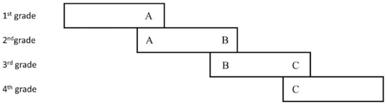
Common-item design.

In the anchor design example in Figure 1, some items in grade 4 are the same as those in grade 3, and some items are the same as those in grade 5. This is called “anchor item.” As a key link of equivalence, “anchor question” is the “miniature version” of the whole test. Generally, the anchor question of grade 4, the link between grade 3 and grade 5 in Figure 1, is more accurate if it accounts for a larger percentage of the whole test. However, in practical application and item bank construction, the more anchor items are used, the following problems will arise: on the one hand, the more anchor items are used, the greater the overall number of items in the item bank will be required, thus increasing the cost of item bank construction; on the other hand, the more anchor items are used, the more proportion of anchor items exposed, and the lower the security and confidentiality of the test. Therefore, it is meaningful to explain the results of vertical equating that how to “set” the proportion of anchor items in an appropriate range for grade span.

Ito et al. (2008) explored the influences of base grades and believed that the selection of different benchmark grades has an impact on the accuracy of evaluation. Hanson and Béguin (2002) examined the separation of grade distributions and drew a conclusion that the separation of grade distributions has an impact on the accuracy of vertical scaling estimation and the higher the grade dispersion is, the lower the accuracy of vertical scaling estimation is. Kolen and Brennan (2014) investigated the proportion of anchor items in a test and suggested the rule of thumb that a common item set should be at least 20% of the length of a total test containing 40 or more items, unless the test is very long, in which case 30 common items might suffice. However, the following problems still exist in the current research literature on the anchor items’ proportion of vertical equating.

Firstly, what is the appropriate anchor items’ proportion for the equivalent test between grades? Relevant evidence is still lacking. At present, most of the research literature on the proportion of anchor items is concentrated in the “horizontal equating” literature (Cai et al., 2009; Meng, 2015). For example, Cai et al. (2009) found in the horizontal equivalence that the proportion of anchor items can be over 18.33% when emphasizing the authenticity of the equivalence coefficient. When emphasizing the equivalent accuracy of the test score system or ability parameter system, the proportion of anchor items can be over 14.29%, or even over 16.67%. Generally, the proportion of anchor items in international large-scale education assessment projects such as PISA, NAEP and TIMSS is at least 20%. The subtest composed of “anchor items” is representative, almost a “miniature” of the entire test (Wang et al., 2014). However, what is the appropriate proportion of anchor items for the vertical equating among the relevant grades? There is still a lack of relatively mature research literature to give a basic conclusion.

Secondly, does the proportion of anchor items with vertical equating between grades change with the growth of grades? Still it is unknown. Because the distribution of the difficulty of tests in adjacent grades is more similar to that of the ability of the subjects, there is more overlapping knowledge between the tests, and the links between the two grades can provide more information. However, with the increase of grade span, the difference between the difficulty of the test and the ability of the subjects becomes larger, and the overlapping content between tests becomes less, which reduces the “strength” of links between grades (Martineau, 2004, 2006). According to this, the anchor items’ proportion setting of vertical equating between grades may change with the growth of grades. In other words, the proportion of anchor items for the vertical equating between grades may not be fixed, and may affect the vertical equating together with the separation of grade distributions. The separation of grade distributions refers to the degree of difference between the abilities of students in different grades. The greater the separation of grade distributions is, the greater the difference among the abilities of students in different grades is, and vice versa.

However, as the span of grades needed to scaling expands, the variance of test difficulty and students’ ability increases, and the overlap contents also reduce so that the linking power falls off and the developmental score scale lacks reliability to interpret the real development. In addition, as a key part of the vertical equating the common item is a miniature of the entire test. Generally speaking, the greater the ratio of common items in the overall test, the more accurate the equivalent coefficient we can expect. However, in the actual construction and application of the item bank, larger number of common items causes larger item bank, which will definitely increase construction cost. A more serious concern is that the more anchors are exposed, the lower the confidentiality and security of the test. When conducting the horizontal scaling or equating, it is suggested that the anchor ratio had better be 25% to 33.33% (Cai et al., 2009; Xiong et al., 2010). However, there is no relevant research on the setting of the common item in vertical scaling, and the standard of horizontal equating is still borrowed. In addition, in the past research, researchers have habitually chosen the middle grade as the base grade, but what is the relationship between the base grade and each grade, and how to determine the base grade, there is not yet a unified standard. Whether the separation of grade distributions will affect the choice of the base grade is not yet considered too.

Considering the above problems, this study chooses the edge grade as base for the simulation, aiming to explore the influence of the ratio of common items and the separation of grade distributions on the precision of vertical scaling, in an attempt to give feasible suggestions for the practice and promotion of vertical scaling.

Methods

Construction Methods

Vertical scaling construction includes three major steps. First of all, calculate the raw score or estimate the ability parameters of candidates on the test. Secondly, which is the most key step, the raw score of each grade is converted to a same scale for comparison. Finally, form a developmental scale by giving interpretations to the scale scores.

In second step, there are three main methods for score conversion, the Thurstone method (Thurstone, 1925, 1938), the Hieronymus method (Peterson et al., 1989), and the IRT method (Meng & Xin, 2014). Compared with the former two methods using the original score, the IRT method uses the item response mode of the candidates of different grades to estimate the ability parameters and item parameters, and then the parameters are converted to the same scale after parameter calibration. In the IRT method, the candidate’s ability parameters and item parameters are independent of the sample. Due to its unique advantages, the IRT method has become the major method for the construction of vertical equating scales (Tong & Kolen, 2007). The IRT-based parameter estimation method can be further divided into concurrent calibration and separate calibration. Practically, concurrent calibration is more convenient to implement because only one operation is needed relatively. Under the circumstance of satisfying the strong assumptions of the IRT theory, the concurrent calibration results are more robust than the separation calibration; otherwise, the separation calibration are better (Béguin & Hansone, 2001; Béguin et al., 2000; Hanson & Beguin, 2002). Therefore, concurrent calibration method was chosen in this simulation study.

Research Design

In this study, we compared various combinations using Monte Carlo simulation. Four grade level tests were administered to first to fourth grade students. Each test contained 100 dichotomous items, and the number of students in each grade was 1,000. We used the common-item design allowing a number of common items to exist between any two adjacent grades. We compare the influence of different anchor items’ proportion and separation of grade distributions on the bias and RMSE value of different grade tests. This study was a 3 × 3 between-subject design and each occasion was repeated 300 times. The independent variable is effect size (ES), which is divided into three levels of 0.5, 1.0, and 1.5 (Student, 2022). Another one is common-item ratio which is divided into three levels of 15%, 30%, and 45%.

Research Instrument

Use R 4.2.2 software to simulate data, item parameters, ability parameters, and response matrix. The BILOG-MG 3.0 software is used to estimate the parameters of the data response matrix, and the equating method used is the simultaneous calibration method (Yildirim, 2014).

Simulation Study

Simulation Design

First grade (lower grade) was chosen as basic reference. Setting 100 items in four grades respectively and 1,000 subjects in each grade, we assume the variation and the degree of separation of distributions between grades are consistent. The separation of distributions in adjacent grades is measured by the effect size (Yen, 1986). It is defined as:

effect size = \frac{\hat{μ} {(Y)}_{upper} - \hat{μ} {(Y)}_{lower}}{\sqrt{\frac{{\hat{σ}}^{2} {(Y)}_{upper} + {\hat{σ}}^{2} {(Y)}_{lower}}{2}}}

(1)

Where $\hat{μ} {(Y)}_{upper}$ and ${\hat{σ}}^{2} {(Y)}_{upper}$ are mean and variance of upper grade, $\hat{μ} {(Y)}_{lower}$ and ${\hat{σ}}^{2} {(Y)}_{lower}$ are mean and variance of lower grade.

Test items are 0/1 scored with two-parameter logistic model to obtain the response matrix of different grade groups on its own grade through Monte Carlo simulation.

Data Generation

Data collection is obtained through data simulation. In order to simulate data, it is necessary to preset the data distribution of each parameter (Kolen, 2003; Tong & Kolen, 2007), as shown in Table 1.

Table 1.

Data Distribution of Parameters.

ES	a	b ₁	b ₂	b ₃	b ₄	θ ₁	θ ₂	θ ₃	θ ₄
0.5	(1, 0.6)	(0, 1)	(0.5, 1)	(1, 1)	(1.5, 1)	(0, 1)	(0.5, 1)	(1, 1)	(1.5, 1)
1.0	(1, 0.6)	(0, 1)	(1, 1)	(2, 1)	(3, 1)	(0, 1)	(1, 1)	(2, 1)	(3, 1)
1.5	(1, 0.6)	(0, 1)	(1.5, 1)	(3, 1)	(4.5, 1)	(0, 1)	(1.5, 1)	(3, 1)	(4.5, 1)

In Table 1, the discrimination parameter follows the log-normal distribution, the difficulty parameters follow the normal distribution, and the ability parameters follow the normal distribution. The mean and standard deviation are indicated in parentheses for each parameter. We used R 3.0 to simulate the student’s response matrix. The following example is the procedure when the ratio of common items is 30%.

For the base grade (first grade), set the mean (μ₁) and variance (δ₁) of ability parameters, the variance of the ability parameters of the remaining grades equal to 1, and the effect size of the adjacent grades is set to 0.5, 1.0, or 1.5, respectively. Thus, the average ability value of each grade can be calculated through Equation 1. The A constants get its values in range [0.7, 1.5] with the step size of 0.1 while B constants are in range [−0.6, 1] and the step size is 0.2. Three pairs of A and B that randomly generated are selected as the equivalent constants of first grade to second grade, second grade to third grade, and third grade to fourth grade which are coded as A₁₂/B₁₂, A₂₃/B₂₃, and A₃₄/B₃₄ accordingly. Since the initial simulation of the ability parameters of each grade is on the same scale as the base grade, it is necessary to convert the ability values of second grade, third grade, and fourth grade to their own grades. The conversion expressions of three grades are as follows:

θ_{2} = A_{12} * θ_{2}^{*} + B_{12}

(2)

θ_{3} = (A_{12} * θ_{3}^{*} + B_{12}) * A_{23} + B_{23}

(3)

θ_{4} = [(A_{12} * θ_{4}^{*} + B_{12}) * A_{23} + B_{23}] * A_{34} + B_{34}

(4)

We hypothesize the difficulty parameter of each grade have normal distribution, and its mean and variance are consistent with the ability parameters of each grade. The discrimination parameters have log-normal distribution, $a_{i j} Lognormal (0, 1)$ . Thirty items are randomly selected from 100 items to form the common items for first grade and second grade.

For the second grade, simulate 70 independent items relative to first grade and then convert the parameters of common items to second grade. Another 30 items are randomly chosen as the common items for second and third grade. For the third grade, the process is the same as the second grade. For the fourth grade, we only need to simulate 70 independent items and then convert their parameters with common items to the fourth grade.

After getting the response matrix, item and ability parameters are estimated with concurrent calibration using EAP algorithm in BILOG 3.0 (Mislevy & Bock, 1990).

Evaluation Criteria

Root mean square error (RMSE) and Bias are used as the criteria to determine the precision of vertical scaling. RMSE measures the systematic error between the estimated value and the true value. Bias is mainly used to detect whether the study contains systematic errors and the direction of the deviation. They are calculated using following expressions:

RMSE = \frac{1}{N} \sum_{n = 1}^{N} \sqrt{\frac{1}{R} \sum_{r = 1}^{N} {({\hat{τ}}_{r} - τ_{r})}^{2}}

(5)

Bias = \frac{\sum_{r = 1}^{R} \sum_{n = 1}^{N} ({\hat{τ}}_{r} - τ_{r})}{R \times N}

(6)

Where R is the number of items, N is the number of repetition, $τ_{r}$ is the true value of parameter, ${\hat{τ}}_{r}$ is the estimate of parameter.

Results

Table 2 shows the summary of means and standard deviations of item and ability parameters, where a1 to a4 represent the discrimination parameters of first grade to fourth grade. Under each condition, the means of the discrimination parameters of each grade are close to 1, and the standard deviations approach 0.6. The b1 to b4 represents the difficulty parameter of first grade to fourth grade. The standard deviations of each grade close 1, and the means of the difficulty parameter increase with the grade. In the case of the same effect size, the average difficulty level of each grade decreases with the increase of the common-item ratio. However, when the effect size is 1.5, the standard deviation of difficulty parameters increases as the proportion of common items increases except for first grade. The θ1 to θ4 represents the ability parameters of first grade to fourth grade. The overall mode is the same as the difficulty parameter, that is, the standard deviation of each grade is close to 1 while in the base grade (first grade), the means of the ability approach 0 and gradually increases as grades rise.

Table 2.

Means and Standard Deviation of Parameters in Each Condition.

ES	ratio		a1	a2	a3	a4	b1	b2	b3	b4	θ1	θ2	θ3	θ4
0.5	15%	M	0.9327	0.9160	0.9519	0.9577	0.0124	0.4530	0.9800	1.4330	−0.0021	0.4965	1.0036	1.4922
		SD	0.5975	0.5849	0.6024	0.6200	0.9956	0.9877	1.0254	0.9950	0.9802	0.9821	0.9797	0.9794
	30%	M	0.9682	0.9510	0.9587	0.9405	0.0337	0.3683	0.8790	1.3461	−0.0092	0.4918	1.0058	1.5100
		SD	0.6113	0.6054	0.6097	0.6040	0.9675	1.0146	1.0038	1.0283	0.9817	0.9838	0.9893	.9866
	45%	M	0.9481	0.9478	0.9674	0.9645	−0.0097	0.2544	0.7386	1.2899	−0.0175	0.4976	0.9928	1.5026
		SD	0.5944	0.6004	0.6078	0.6077	0.9967	0.9968	0.9923	1.0157	0.9873	0.9864	0.9823	0.9891
1.0	15%	M	0.9361	0.9210	0.9483	0.9547	0.0073	0.8764	1.9054	2.8593	−0.0027	0.9978	2.0055	2.9925
		SD	0.5993	0.5867	0.5994	0.6178	0.9871	1.0333	1.0645	1.0355	0.9799	0.9800	0.9796	0.9794
	30%	M	0.9682	0.9510	0.9587	0.9405	0.0337	0.7183	1.7290	2.6961	−0.0092	0.9918	2.0058	3.0100
		SD	0.6113	0.6054	0.6097	0.6040	0.9675	1.0846	1.0762	1.1045	0.9817	0.9838	0.9893	0.9866
	45%	M	0.9426	0.9557	0.9653	0.9610	−0.0090	0.5243	1.5186	2.5733	−0.0190	0.9968	1.9930	2.9992
		SD	0.5928	0.6065	0.6115	0.6085	0.9997	1.0916	1.0837	1.1102	0.9874	0.9865	0.9859	0.9876
1.5	15%	M	0.9277	0.9203	0.9566	0.9600	0.0060	1.2957	2.8298	4.2930	−0.0033	1.4974	3.0035	4.4935
		SD	0.5950	0.5872	0.6021	0.6201	0.9858	1.1131	1.1410	1.1060	0.9783	0.9813	0.9828	0.9802
	30%	M	0.9673	0.9576	0.9602	0.9419	0.0351	1.0772	2.5804	4.0361	−0.0079	1.4915	3.0058	4.5095
		SD	0.6100	0.6056	0.6089	0.6065	0.9642	1.1951	1.1933	1.2196	0.9813	0.9841	0.9891	0.9849
	45%	M	0.9426	0.9557	0.9653	0.9610	−0.0090	0.7993	2.2936	3.8483	−0.0190	1.4968	2.9930	4.4992
		SD	0.5928	0.6065	0.6115	0.6085	0.9997	1.2237	1.2202	1.2482	0.9874	0.9865	0.9859	0.9876

Table 3 is the summary of Bias and RMSE of item and ability parameters under each condition. Note that when the effect size is 1.5 and the common-item ratio is 45%, the estimation can’t converge. In order to display the trend of the Bias and RMSE values of each grade under different conditions more clearly, Figures 2 to 7 are the line graph which the horizontal axis is different conditions (effect size-common item ratio), and the vertical axis is the Bias or RMSE value.

Table 3.

Bias and RMSE Value of Parameters in Each Condition.

ES	ratio		a1	a2	a3	a4	b1	b2	b3	b4	θ1	θ2	θ3	θ4
0.5	15%	Bias	0.0174	−0.0029	0.0057	0.0315	0.0065	0.0255	0.0413	−0.1294	−0.0021	0.0135	0.0370	−0.1866
		RMSE	0.8259	0.1084	0.1308	0.1419	0.1908	0.1520	0.1712	0.4813	0.2441	0.1947	0.2177	0.5529
	30%	Bias	0.0143	0.0075	0.0071	0.0189	−0.0107	−0.0115	−0.0107	−0.0745	−0.0092	−0.0171	−0.0222	−0.1342
		RMSE	0.0948	0.0909	0.0894	0.1918	0.1140	0.1141	0.1113	0.4487	0.1765	0.1842	0.1845	0.5556
	45%	Bias	0.0204	0.0209	0.0100	0.0379	−0.0180	−0.0367	−0.0639	−0.3539	−0.0035	−0.0430	−0.0780	−0.6125
		RMSE	0.1110	0.1108	0.0977	0.1552	0.1411	0.1442	0.1467	0.5260	0.1817	0.2408	0.2143	0.7251
1.0	15%	Bias	0.0227	0.0190	0.0453	0.0819	−0.0105	−0.0674	−0.1026	−0.3505	−0.0027	−0.0980	−0.1239	−0.4182
		RMSE	0.1360	0.1143	0.1556	0.1722	0.2015	0.2150	0.2839	0.7828	0.2449	0.2677	0.3334	0.7773
	30%	Bias	0.0152	0.0157	0.0293	0.0350	−0.0112	−0.0338	−0.0670	−0.1854	−0.0092	−0.0319	−0.0658	−0.2713
		RMSE	0.0946	0.1284	0.1456	0.3881	0.1143	0.1854	0.2092	0.7231	0.1767	0.1920	0.2112	0.7143
	45%	Bias	0.0147	0.0225	0.0240	0.0469	−0.0217	−0.0373	−0.0703	−0.5288	−0.0190	−0.0588	−0.1046	−0.8144
		RMSE	0.0944	0.0878	0.1024	0.1785	0.1256	0.1144	0.0946	1.1108	0.1818	0.1997	0.2313	0.8867
1.5	15%	Bias	0.0217	0.0127	0.0649	0.0080	−0.0015	−0.0105	−0.1087	−0.1618	−0.0033	−0.0321	−0.1067	−0.2168
		RMSE	0.0980	0.1003	0.1656	0.2237	0.1333	0.1416	0.5006	0.6668	0.1824	0.1964	0.2837	0.6878
	30%	Bias	0.0168	0.0303	0.0643	0.0630	−0.0130	−0.0259	−0.1085	−0.3028	−0.0079	−0.0455	−0.1581	−0.3388
		RMSE	0.0964	0.1026	0.1426	0.1887	0.1147	0.1299	0.2952	1.0911	1.1461	0.2054	0.2844	0.8754
	45%	Bias	NA	NA	NA	NA	NA	NA	NA	NA	NA	NA	NA	NA
		RMSE	NA	NA	NA	NA	NA	NA	NA	NA	NA	NA	NA	NA

Figure 2.

Line chart of bias of discrimination parameters under different conditions.

Figure 3.

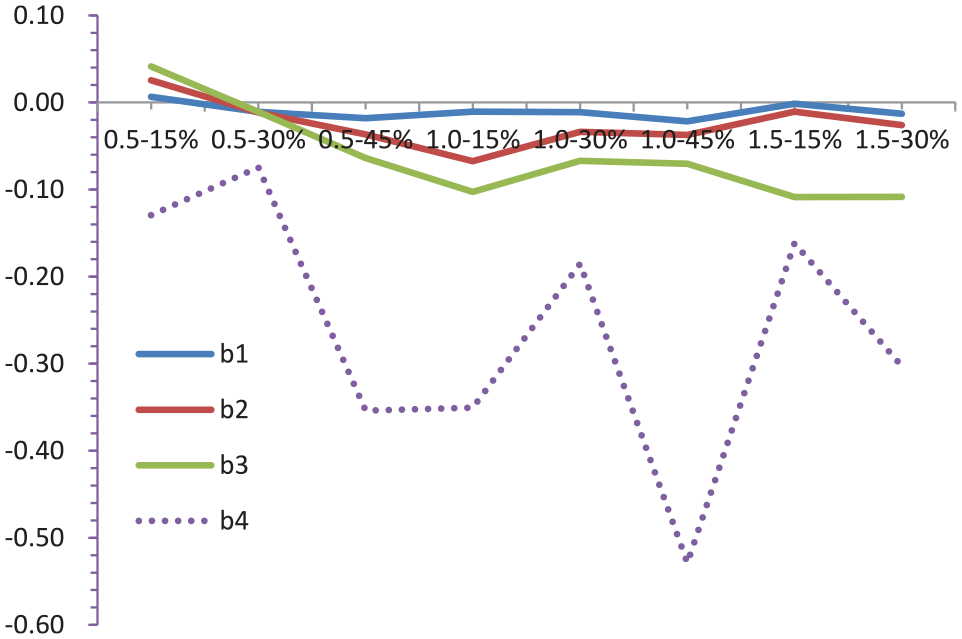
Line chart of bias of difficulty parameters under different conditions.

Figure 4.

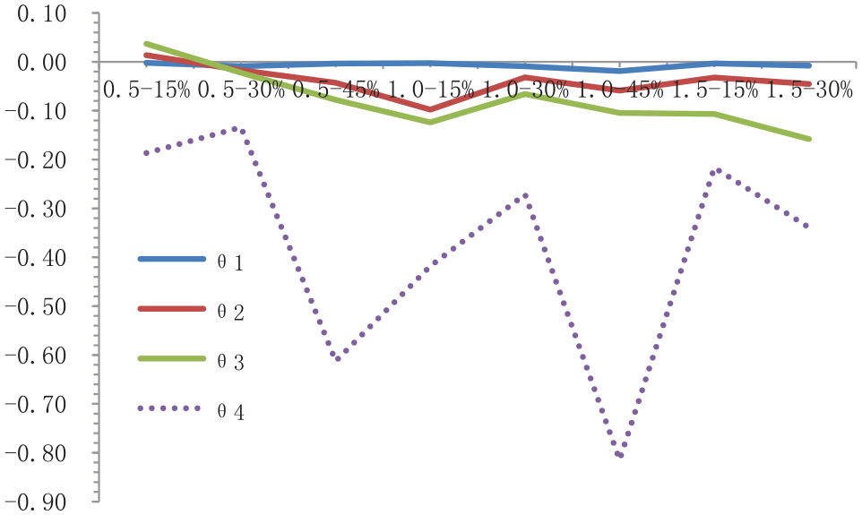
Line chart of bias of ability parameters under different conditions.

Figure 5.

Line chart of RMSE of discrimination parameters under different conditions.

Figure 6.

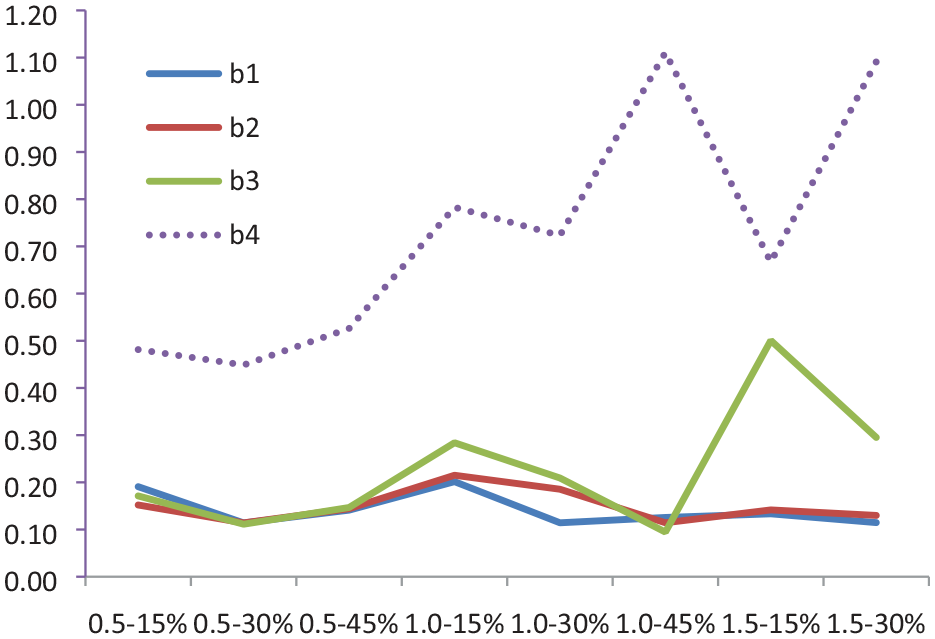
Line chart of RMSE of difficulty parameters under different conditions.

Figure 7.

Line chart of RMSE of ability parameters under different conditions.

Analysis of Bias

As shown in Figure 2, the chart indicates that the estimated discrimination parameters are overall larger than the true value except for second grade when the effect size is 0.5% at 15% of common-item ratio. Overall, the Bias of discrimination parameter presents an unstable trend. When the effect size is 0.5, the Bias of each grade gets smallest value at 30% of common-item ratio. When the effect size is 1.0, the Bias of first grade is lower at 15% of anchor ratio than when the anchor ratio is 30% and 45%; and for second grade and fourth grade it is at 30% to get smallest Bias; but for third grade the best common-item ratio is 45%. When the effect size is 1.5, the estimated parameters do not converge at 45% of common-item ratio. Comparing the common-item ratio 15% and 30%, except for the first grade that the Bias is smaller at 30% than 15% of common-item ratio, the Bias is smaller at 15% than 30% for other grades. Besides, the Bias of first grade and second grade is much smaller than that of third grade and fourth grade. Comparing the Bias under same common-item ratio, there is no obvious pattern under different effect sizes in each grade.

As seen from Figure 3, except for the first, second, and third grade when the effect size is 0.5 at 15% of common-item ratio, the estimated value of the difficulty parameter is lower than the true value. In addition, as the grade increases, the Bias goes up and the growth rate is biggest at fourth grade, which reveals that the farther away from the base year, the greater the equating error. When the effect size is 0.5 and 1.0, except for first grade getting smallest Bias at 15% of the common-item ratio, the Bias is smallest at 30% on other grades; when the effect size is 1.5, the Bias has the smallest value at 15% of common-item ratio except for third grade.

As shown in Figure 4, most estimates are smaller than the true value. When the effect size is 0.5, the first grade and second grade have the smallest Bias at 15% of common-item ratio, but at 30% for third grade and fourth grade. When the effect size is 1.0, the first grade gets smallest Bias at 15% while at 30% for the other grades. When the effect size is 1.5, all the grades have the smallest Bias when the common-item ratio is 15%. Besides, as the grade rises, the Bias increases and the growth rate is greatest at fourth grade which indicates the farther away from the base year, the greater the equivalent error.

Analysis of RMSE

Figure 5 is a line chart of the RMSE value of each grade discrimination parameter under different conditions. The RMSE of first grade is generally smaller than 0.5 except for under the effect size of 0.5 at 15% of common-item ratio. The lines of the first grade and second grade are nearly paralleled. The RMSE of third grade rises with the increase of the effect size, and by fourth grade the estimation accuracy decreases more sharply. Therefore, it is easy to find that the farther away from the base grade, the lower the estimation accuracy.

As for the common-item ratio, when the effect size is 0.5 and 1.0, the fourth grade has the lowest estimation accuracy at 30% of the common-item ratio. For the other grades, the accuracy is highest at 30% and 45% of the common-item ratio when the effect size is 0.5 and 1.0, respectively. Since the estimation doesn’t converge when the common-item ratio is 45% and effect size is 1.5, we can only compare two conditions, which is obvious that less than 30% of common-item ratio is better. In general, when the effect size is 0.5, the estimated error is the smallest; while when the effect size is 1.0 and 1.5, the result is not stable and fluctuates greatly at each grade.

Figure 6 is a line chart of the RMSE values of the difficulty parameters of each grade under different conditions. In general, the RMSE values of each grade are of little difference except for fourth grade. The lines of first grade and second grade are nearly paralleled, and the estimation error of third grade rises with the increase of effect size; when the degree of effect size is 1.5, the increase of estimation error becomes larger. Overall, when the effect size is 0.5, the estimation accuracy is the highest, and as the separation of grade distributions increases, the estimation accuracy decreases. When the effect size is 1.5, the estimation accuracy is rather unstable, and there are even cases where the data cannot converge.

As for the common-item ratio, the accuracy is highest at 30% when the separation of grade distributions is 1.5; while when the separation of grade distributions is 1.0, the accuracy is highest at 45% except for fourth grade which is better at 30%. Since the estimation doesn’t converge at 45% of common-item ratio when effect size is 1.5, we can only compare two conditions, which interestingly show that less than 30% of common-item ratio is better except for fourth grade which is better at 15%.

Figure 7 is a line chart of the RMSE values of the ability parameters of each grade under different conditions. Generally, the RMSE values of each grade are of little difference except for fourth grade which is much larger. Surprisingly, the RMSE value of first grade goes extreme at 30% of common-item ratio when the separation of grade distributions is 1.5. The accuracy is highest at 0.5 of effect size and declines as the separation of grade distributions goes up. However, it is found that the accuracy of higher separation (1.5) is better than lower separation (1.0) when the common-item ratio is 15%. But later in higher separation when the ratio rises to 30%, the accuracy decreases and the data cannot converge at 45%.

In general, when the separation of grade distributions is 0.5 and 1.0, the estimate precision is best at 30% of common-item ratio. However, when the separation of grade distributions is 1.5, the precision is best at 15%.

Discussions

Analysis of Items and Ability Parameters for Vertical Scaling

In Table 2, the average difficulty parameters increase with the grade, which is logical and common. In general, with the grade rising, the difficulty of the items is set higher and higher. However, in the case of the same effect size, the average difficulty of each grade decreased with the increase of the proportion of anchor items, which is consistent with the result of Bjermo and Miller (2021). In Table 2, the average ability of the subjects in the base grade (grade 1) tends to be 0, and the average ability of the subjects in other grades gradually increases, which reflects that the ability of the subjects in each grade is gradually increasing, which is similar to that of Sari and Kelecioğlu (2016).

The results in Table 2 show that the parameter values (i.e., true values) are basically consistent with the set data distribution characteristic values (see Table 1), which indicates that the data simulation method is reliable, which lays a foundation for subsequent analysis to generate the original score response matrix of the subjects, and then to estimate the discrimination parameters, difficulty parameters, and ability parameters.

Parameters and Bias Values of Each Grade

Bias reflects the difference between estimate and true value. In this study, the Bias value of all parameters increases with the grade going up especially at fourth grade which rises sharply. For the RMSE, it is also found this trend. The vertical scaling under common-item design is a cumulative conversion because the common items are between adjacent grades so that the parameters of fourth grade needs to be conversed grade by grade three times, which definitely accumulates estimation errors. Since this cumulative effect exits, researchers normally choose middle grade as base grade to decrease the errors (Guo, 2014; Yen et al., 2012). In our study, we didn’t choose middle grade but edge grade to explore how this cumulative effect behaves. The result indicates that the number of conversion should not exceed two times for keeping the precision of vertical scaling.

It can be seen from Table 3 that when the effect size is 1.5 and the proportion of anchor items is 45%, the data does not converge, which shows that with the growth of grades, for the more anchor items increase, the worse the effect of the vertical equating and common items of students’ abilities between grades (until the data cannot converge), which is logical. Generally, there is a big gap between the abilities of students in grade 1 and that of students in grade 4. If there are too many common items (anchor items) at this time, the effect of vertical equating is poor, which directly leads to the difficulty of vertical equating and the ultimate failure (i.e., “NA” in Table 3 of this paper).

It can be seen from the results in Figures 2 to 4 that with the growth of grade, the value of bias of vertical equating is getting larger and larger. Among them, the broken lines of bias values between grade 1 and grade 2 are basically parallel, while bias value of grade 3 gradually increases with the increase of the effect value, and bias value of grade 4 decreases significantly with the increase of the effect value. This fully reflects that the further away from the base grade, the lower the estimation accuracy. The difference among grade 1, grade 2, and grade 3 is relatively small, but by grade 4, the value of bias is already too large to accept (it can be seen from the dotted lines in Figures 2 to 4. Therefore, if the lower grade is selected as the base grade, if the number of consecutive cumulative conversions exceeds 2 in the process of converting the test scores of the upper grade to the lower grade, there will be a large deviation. In this view, if the senior grade is converted to the junior grade, it is suggested that the gap between the reference grade and the senior grade should not exceed two grades. Otherwise, the resulting vertical equating bias value is unacceptable.

Parameters and RMSE Values of Each Grade

In general, the results further indicate that effect size and common-item ratios interact with each other since they behave inconsistently.

For the effect size of 0.5, the estimated precision of discrimination parameters under different common-item ratios are of little difference between first and second grade but not between third and fourth grade. For third grade, the estimated precision at 30% and 45% of common-item ratio is higher than that of 15%; while for fourth grade, estimated precisions of each ratio are quite different and the highest precision that getting at 15% is still lower than the lowest precision of third grade. Therefore, the common-item ratio should be 30% when the effect size is 0.5 to ensure a most accurate discrimination parameter. As for the difficulty parameter, the difference of estimated precision under different common-item ratios is more than that of discrimination parameter. Specifically, the precision at 30% is much higher than 45% and 15% and even for fourth grade whose precision is much lower than the other grades. Since the ability parameter has the same distribution of difficulty parameter, their conclusions are quite similar so we don’t further discuss here. In summary, we suggest that the common-item ratio should be 30% when the separation of grade distributions is 0.5.

For the effect size of 1.0, the precision of discrimination parameter increases as the common-item ratio rising up. For first grade, the estimated precisions at 30% and 45% are of same level but obviously higher than that of 15%; for second and third grade, estimated precision at 45% is much higher than other ratios. However, the precision of difficulty parameter makes a bit difference under different conditions. For first grade, the estimated precisions (mainly RMSE) at 30% is a little better than that of 45% while for second and third grade 45% is the best ratio. As for fourth grade, precision at 30% is a little higher than that of 15%. In terms of ability parameters, the estimated precision is highest at 30% of all grades, although the difference between 30% and 45% is less than 0.2. Thus common-item ratio should better be 30% considering the balance between precision and practice (Wyse & McBride, 2022).

For the effect size of 1.5, the data cannot converge at 45% of common-item ratio, which means the ratio should not be too large when student’s ability has a large growth. As for discrimination parameter, the precision at 15% and 30% is not much different although 30% is slightly better. Similarly, difficulty parameter is best estimated at 30% of common-item ratio except for fourth grade that is at 15%. As for ability parameters, the most accurate ratio is 15%. The above indicates that if the current grade is two or more grades away from base grade, the common-item ratio should reduce in order to get a better estimation, or in other words, the gap of conversion should not exceed two grades. Therefore, we suggest that when the effect size is 1.5, 30% of common-item ratio is better if we care more about item parameters otherwise 15% is better if we need a more accurate ability parameter. In equating practice, former researchers recommend that the common-item ratio should between 25% and 33.33% (Cai et al., 2009), but how to set common-item ratio in vertical scaling is lack of relevant research therefore the standard of equating is adapted temporally.

Overall, when the separation of grade distributions is 0.5 and 1.0, the effect of equivalent precision is the best when the proportion of anchor items is 30%. However, when the separation of grade distributions is 1.5, the estimation accuracy is the best when the anchor question proportion is 15%.

This research attempts to find criteria for setting common-item ratio in vertical scaling. According to previous researches, the growth rate of student’s ability changes as the grade rising up. Also in this study, it is found that common-item ratio interacts with effect size which means we need to adjust common-item ratio according to the effect size between adjacent grades but not choose a fixed ratio in large scale testing (Briggs & Dadey, 2015; Briggs & Peck, 2015). As for the different behaviors between item parameter and ability parameter on certain common-item ratios, further studies need to continue such as narrowing the gap of ratios to find out the balance point for best estimated precision of item parameters and ability parameters.

Limitations

First of all, only the lower grade is considered as the base, and there is no further analysis of the middle or higher grade as the base. Secondly, the distribution of anchor question parameters considered does not change between different grades, which are different from Sari and Kelecioğlu (2016). Thirdly, the assumed grade dispersion and test length are the same among different grades and do not change, which is different from the practices (Xiong et al., 2010). Last but not least, the project parameter calibration/estimation method is only limited to the simultaneous calibration method and other methods such as separate calibration and fixed common problem parameter calibration are not considered.

Conclusions

Estimation precision of item and ability parameters differs in each grade. For discrimination and difficulty parameters, estimation precision is higher as closer to the base grade. For the ability parameters, the estimation precision of item parameter decreases with the increase of effect size, especially much lower in fourth grade. There is an interaction between the ratio of common items to total test, effect size and the interval from base grade. When the effect size was 0.5 and 1.0, estimation precision of each grade is accurate at 30% of common-item ratio. When the effect size is 1.5, the estimation precision is best for first, second, and third grade at 30% of common-item ratio while grade 4 at 15% of common-item ratio. The selection of base grade affects the precision of vertical scaling. So, we recommend that the interval of scaling should not exceed two grades from the base grade. As a whole, the proportion of anchor items for vertical scaling is set at 30%, and the equivalent effect is relatively best. But the setting of the proportion of anchor items is affected by the separation of grade distributions, and there is an interaction between them. So, it is better to set the proportion of anchor items as “variable” value (15%–30%).

Footnotes

Author Contributions

Each author has contributed significantly to the work and agreed to the submission.

Declaration of Conflicting Interests

The author(s) declared no potential conflicts of interest with respect to the research, authorship, and/or publication of this article.

Funding

The author(s) disclosed receipt of the following financial support for the research, authorship, and/or publication of this article: This research was supported in part by Grant No. 18YJA190006 from the Ministry of Education Foundation of the People’s Republic of China.

ORCID iD

Guangming Li

Data Availability Statement

The datasets used and/or analyzed during the current study are available from the author on reasonable request.

References

Béguin

A. A

Hanson

B. A.

(2001). Effect of non-compensatory multidimensionality on separate and concurrent estimation in IRT observed score equating [Paper presentation]. Annual Meeting of the National Council on Measurement in Education, Seattle, WA.

Béguin

A. A.

Hanson

B. A.

Glas

C. A. W.

(2000). Effect of multidimensionality on separate and concurrent estimation in IRT equating [Paper presentation]. Annual Meeting of the National Council of Measurement in Education, New Orleans, LA.

Bjermo

Miller

(2021). Efficient estimation of mean ability growth using vertical scaling. Applied Measurement in Education, 34(3), 163–178.

Bolt

D. M.

Deng

Lee

(2014). IRT model misspecification and measurement of growth in vertical scaling. Journal of Educational Measurement, 51(2), 141–162.

Briggs

D. C.

Dadey

(2015). Making sense of common test items that do not get easier over time: Implications for vertical scale designs. Educational Assessment, 20(1), 1–22.

Briggs

D. C.

Peck

F. A.

(2015). Using learning progressions to design vertical scales that support coherent inferences about student growth. Measurement Interdisciplinary Research & Perspectives, 13(2), 75–99.

Cai

Ding

(2009). The effect of the ratio of anchor items to total test on the precision of equating. Psychological Exploration, 110(2), 56–59.

Dadey

Briggs

D. C.

(2012). A meta-analysis of growth trends from vertically scaled assessments. Practical Assessment Research and Evaluation, 17(14), Article 14.

Dai

Zhang

(2018). Psychological and educational measurement (4th ed.). Jinan University Press.

10.

Guo

(2014). The different base group and separation of grade distribution on the influence of vertical scaling [Unpublished dissertation]. Jiangxi Normal University.

11.

Hanson

B. A.

Béguin

A. A.

(2002). Obtaining a common scale for item response theory item parameters using separate versus concurrent estimation in the common-item equating design. Applied Psychological Measurement, 26(1), 3–24.

12.

Ito

Sykes

R. C.

Yao

(2008). Concurrent and separate grade-groups linking procedures for vertical scaling. Applied Measurement in Education, 21(3), 187–206.

13.

Kolen

M. J.

(2003). Equating and vertical scaling: Research items [Paper presentation]. Annual Meeting of the National Council on Measurement in Education. Chicago.

14.

Kolen

M. J.

Brennan

R. L.

(2004). Test equating, scaling, and linking: Methods and practices (2nd ed.). Springer-Verlag.

15.

Kolen

M. J.

Brennan

R. L.

(2014). Test equating, scaling, and linking: Methods and practices (3rd ed.). Springer-Verlag.

16.

Martineau

J. A.

(2004). The effects of construct shift on growth and accountability models [Unpublished doctoral dissertation]. Michigan State University.

17.

Martineau

J. A.

(2006) A distorting value added, the use of longitudinal, vertically scaled student achievement data for growth-based, value-added accountability. Journal of Educational and Behavioral Statistics, 31(1), 35–62.

18.

Meng

Y. E.

(2015). Research on the representativeness of anchor items in test links. Psychological Science, 38(1), 209–215.

19.

Meng

Xin

(2014). Effects of item parameter drift on vertical scaling with the nonequivalent groups with anchor test (neat) design. Educational & Psychological Measurement, 74(2), 227–235.

20.

Mislevy

R. J.

Bock

R. D.

(1990). BILOG 3: Item analysis and test scoring with binary logistic models [Computer program]. Scientific Software.

21.

Nicewander

Sukin

Goodman

Dodson

Schulz

Lottridge

Winter

(2013). Developmental scale for North Carolina end-of-grade/End-of-course ELA/reading and English II tests (4th ed.). Pacific Metrics Corp.

22.

Petersen

I. T.

Lindhiem

LeBeau

Bates

J. E.

Pettit

G. S.

Lansford

J. E.

Dodge

K. A.

(2018). Development of internalizing problems from adolescence to emerging adulthood: Accounting for heterotypic continuity with vertical scaling. Developmental Psychology, 54(3), 586–599.

23.

Peterson

N. S.

Kolen

M. J.

Hoover

H. D.

(1989). Scaling, norming, and equating. In Linn

R. L.

(Ed.), Educational measurement (3rd ed., pp. 221–264). Macmillan.

24.

Ræder

H. G.

Andersson

Olsen

R. V.

(2022). Numeracy across grades-vertically scaling the Norwegian national numeracy tests. Assessment in Education: Principles, Policy & Practice, 29(6), 653–673.

25.

Sari

A. A.

Kelecioğlu

(2016). Assessment of achievement and growth by vertical scaling: Comparison of vertical scaling methods. Journal of Educational Sciences Research, 6(2), 25–38.

26.

Shen

(2014). On the influence of socioeconomic status on children’s academic development. Educational Research, 9(4), 70–76.

27.

Student

S. R.

(2022). Vertical scales, deceleration, and empirical bases for growth. Educational Researcher.

28.

Thurstone

L. L.

(1925). A method of scaling psychological and educational tests. The Journal of Educational Psychology, 16(7), 433–451.

29.

Thurstone

L. L.

(1938). Primary mental abilities. Psychometric Monographs, 1, ix+121.

30.

Tong

Kolen

M. J.

(2007). Comparisons of methodologies and result in vertical scaling for educational achievement tests. Applied Measurement in Education, 20(2), 227–253.

31.

Wang

Bian

Xin

(2011). Vertical scaling: The development and application. Psychological Exploration, 31(5), 472–476.

32.

Wang

Tang

Liu

Zhang

(2014). The application of IRT and MIRT in test vertical equating. Advances in Psychological Science, 22(5), 881–888.

33.

Wells

C. S.

Subkoviak

M. J.

Serlin

R. C.

(2002). The effect of item parameter drift on examinee ability estimates. Applied Psychological Measurement, 26(1), 77–87.

34.

Wyse

A. E.

McBride

J. R.

(2022). Handling extreme scores in vertically scaled fixed-length computerized adaptive tests. Measurement: Interdisciplinary Research and Perspectives, 20(1), 1–20.

35.

Xiong

Ding

Luo

(2010). Study of common-item ratio in equating design. International Conference on Education Technology & Training, 7, 197–200

36.

(2015). Exploration of performance of plausible values method under different vertical equating [Unpublished dissertation]. Taichung University of Education, Institute of Educational Test Statistics, Taichung.

37.

Yen

W. M.

(1986). The choice of scale for educational measurement: An IRT perspective. Journal of Educational Measurement, 23(4), 299–325.

38.

Yen

W. M.

Lall

V. F.

Lora

(2012). Evaluating academic progress without a vertical scale. Ets Research Report, 1, 1–55.

39.

Yildirim

H. H.

(2014). Findings from an empirical vertical scaling study with BILOG-MG [EB/OL]. Education & Science.

40.

Zhang

Luo

Tao

Luo

Dong

(2015). Family socioeconomic status, parental investment and migrant children’s academic achievement in China. Journal of Psychological Science, 1, 19–26.

The Effect of the Ratio of Common Items and the Separation of Grade Distributions on the Precision of Vertical Scaling

Abstract

Plain language summary

Keywords

Introduction

Methods

Construction Methods

Research Design

Research Instrument

Simulation Study

Simulation Design

Data Generation

Evaluation Criteria

Results

Analysis of Bias

Analysis of RMSE

Discussions

Analysis of Items and Ability Parameters for Vertical Scaling

Parameters and Bias Values of Each Grade

Parameters and RMSE Values of Each Grade

Limitations

Conclusions

Footnotes

Author Contributions

Declaration of Conflicting Interests

Funding

ORCID iD

Data Availability Statement

References