The Effects of the Interactions Between Agro-Production,Economic,and Financial Development on Bank Sustainability

Abstract

The Sub-Saharan African region encounters a deficiency in agricultural financing, which can be attributed to its constraints in accessing international investments in general and the low engagement of bank risk-taking in particular. This situation leads to underproduction, which exacerbates poverty and malnutrition in the region. Thus, this study investigates the impact of the interaction effects between agricultural production, economic development (ED), and financial development (FD via FDI and DC) on bank stability ratios across 40 countries, encompassing 350 operational banks, during the period covering 2010 to 2019. The research employs the Generalized Method of Moments (GMM) technique and verifies its consistency with Two-Stage Least Squares (2SLS) and the Z-Score Approach. The results highlight two findings: first, the interaction effects between economic development, agricultural production, and financial development factors have significantly greater impacts on bank sustainability than their individual effects without interactions. Secondly, these interaction effects sustain significantly bank stability in two ways: on the one hand, they increase bank returns (through both ROE and ROA), while on the other hand, they reduce bank riskiness (via negative effects on NPL and positive effects on LLR). The study concludes that those interaction effects significantly sustain the stability of the African banking system. The SS African states (via their central banks) should promote farming finance services and enforce a minimum ratio of farming loans for each commercial bank’s credit portfolio as a solution to the investment deficiency in the sector. Hence, this can solve food production level issues, ensure food security, and effectively sustain both the banking system and real economic development.

Introduction

The banking sector in developing countries plays an essential role in economic growth by offering credit to private industries and small businesses (Beck & Demirguc-Kunt, 2006; Hoang et al., 2022). The studies of the mutual relationship between economic development (ED) and financial development (FD) are not new (Hicks, 1969; Schumpeter, 2017). One study suggests that these connections are stronger in developing economies than in developed economies (Calderón & Liu, 2003). Scholars and decision-makers manifest growing interest in examining the function of the financial system in emerging economies and evaluating its correlation with economic development from different perspectives (Olorogun et al., 2022). Banks involved in financial services serve as intermediaries in the economic system; crucially, they supply liquidity for innovative investments and production activities (S. Ali et al., 2022; Park & Mercado, 2015). By providing loans, these intermediary institutions affect the overall financial and economic structure (Craig & Ma, 2022).

Financial development (FD) in general, Foreign Direct Investment (FDI), and Domestic Credit (DC) in particular, ensure liquidity flows in the entire economic system and thus help to guarantee bank stability (S. Ali et al., 2022; Levine, 1997; Otchere et al., 2017; Park & Mercado, 2015). The extent of a financial system’s liquidity reflects the size of its business and economic activities, which is a primary measure of ED, especially in developing countries (Levine, 1997; Otchere et al., 2017; Park & Mercado, 2015; Purewal & Haini, 2022). Other studies on the causal effects between the two concerned variables also support this claim (Calderón & Liu, 2003; Masten et al., 2008; Rioja & Valev, 2004).

A comparative study concludes that financial markets have different impacts on developed and developing nations, especially when supported with real production output (Ibrahim & Alagidede, 2018). More financial investments and services are required to facilitate significant positive and economic changes. However, developing countries depend only on meagre local finance and experience a deficiency of funds due to financial access barriers (Papadavid et al., 2017).

The majority of prior research establishes the correlation between ED and FD and only evaluates their co-integration and causality impacts in both the short and long term (Bist & Bista, 2018; Rasool et al., 2021; Samargandi et al., 2015; Tran, 2022). It is noteworthy that recent literature merely indicates the presence of additional advantages arising from the relationship between ED and FD in developing nations, without explicitly describing their specific benefits on distinct economic sectors or elucidating the mechanism models for developing countries (Fung, 2009).

This study supports existing literature on the mutual effects of ED and FD (Bist, 2018; Deidda, 2006) for developing countries. However, it extends existing research in two ways: First, in addition to evaluating their basic causality tests between these two variables (Bist & Bista, 2018; Ibrahim & Alagidede, 2018) and their co-integration movements (Bist & Bista, 2018; Rasool et al., 2021), this study adds a third factor—financial development (FD), represented by domestic credit (DC), and FDI net inflows—and explores how the ED*DC and ED*FDI interaction effects sustain financial stability in ways that benefit the banking sector. And second, as agriculture is the main contributor to the African ED (Suri & Udry, 2022), study also evaluates the role of agriculture production factors (food production and/or cereal production) in the sustainability of the African banking system, especially when interacting with FD factors (Food*DC and food*FDI). Those two points bring new evidence on the role of agriculture and financial development in sustaining the African banking system. The first round involves ED, DC, and FDI, while the second round involves Food-Xo, DC, and FDI, as illustrated in Figure 1.

Figure 1.

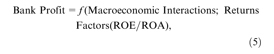
Bank stability as a result of the interaction effects between bank credit (DC), economic growth (ED), and foreign direct investment net inflows (FDI).

In the first round, study evaluates the positive effects of the ED-FD and ED-FDI interaction effects on bank stability in developing countries and showcasing how the complementary relationships between these macro-economic factors impact the sustainability of the banking sector, this work provides new evidences of the join effects in boosting ED in SSA economies, as in following Figures 1 and 2.

Figure 2.

Bank sustainability as a result of the interaction effects between the macroeconomic factors (FDI, ED, and agriculture production with food production as a proxy).

Two studies reveal that African ED is significantly backed by agricultural production (Gollin, 2020; Suri & Udry, 2022), as shown in the evolution trends of Figures 3 and 4.

Figure 3.

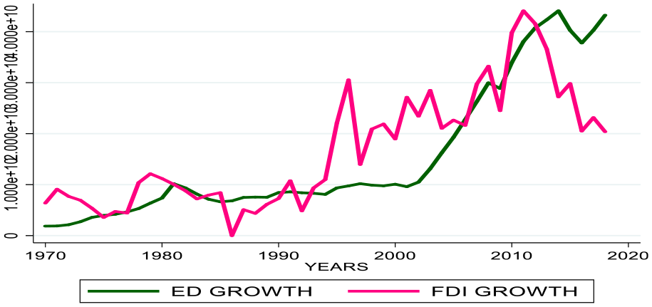
Evolution in scissors effects: FDI and GDP Growth (ED) since 1.

Figure 4.

Evolution of ED Growth and Cereal Production in SSA Africa.

Therefore, in the second round, this study also considers the interaction effects between the agricultural production sector and FD factors (specifically, DC and FDI). It employs food production factor that represents the agricultural production sector to assess the interaction effects between food production and FD factors and their effects on bank stability proxies.

Studies have shown that agricultural production depends on effective food production policies, which depend on many complex developmental plans and strategies, including financial, technical, labor, and environmental policies (Babu & Akramov, 2022). Such public policies determine and define the quantity and quality of agricultural output through crop yield and agriculture production levels, such as cereal production quantity in tons (He et al., 2022; Klerkx & Rose, 2020).

In emerging countries like SS states, agricultural policies primarily respond to deficiencies in food production to meet regional food demand -in terms of both quality and quantity- (Babu & Akramov, 2022). Meeting food demand requires new farming technologies, mechanization, different qualities, and quantities of seeds, smart technologies, and an updated production and transformation system to eliminate underproduction (W. Liu et al., 2021; Yitayew et al., 2022). Such a persistent and resilient agricultural system can eliminate undernourishment, boost agricultural production, and sustain ED and banking in African economies (Kumar et al., 2017; Martin & Clapp, 2015; Suri & Udry, 2022).

Government interventions (including commercial banks) with huge investments in SSA are necessary to increase production (Babu & Akramov, 2022; Jayne et al., 2010). For example, African governments can increase production by implementing policies that channel cash flows into farming in ways that maximize production output and social impact (Kaya & Kadanalı, 2022; Kumar et al., 2017).

By doing so, they can increase underproduction, mitigate unemployment, and poverty and then meet the market demands of SSA’s growing population (Kumar et al., 2017). Furthermore, existing studies attest that a rise in credit, in FDI net inflows, and innovation techniques improve agricultural production, especially cereal production (Chinseu et al., 2022; Ngong, Onyejiaku et al., 2022; Sikandar et al., 2021). Therefore, increasing agricultural financing may improve agricultural production, socio-economic development, and sustain financial system in Africa (Asaleye et al., 2020; Saha & Kasi, 2022).

However, African agricultural challenges are bank credit constraints for farmers (Ogunyiola et al., 2022); lack of credit insurance (Binswanger-Mkhize, 2012); lack of government policies (Yigezu et al., 2018); lack of private sector investments (Yigezu et al., 2018); low mechanization rates (He et al., 2022; Shita et al., 2018); unavailability of new technologies, such as “geo-farming” (Eitzinger et al., 2019; Büntgen et al., 2021); and poor quality innovation (Ananth et al., 2006). African governments ought to consider these significant challenges and construct strategies to enhance agricultural productivity, promote ED, and mitigate poverty (Shita et al., 2018; Sikandar et al., 2021) (Figure 5).

Figure 5.

Evolution of cereal and food production in SS Africa.

In the second round, study examines the interactions between FD factors and agriculture production. On one side, FD influences both ED and agro-production (Ngong, Thaddeus et al., 2022). On the other side, ED has an impact on bank risk and credit in general (F. Abbas et al., 2021; Ding & Sickles, 2019; Joaqui-Barandica et al., 2022), as well as on bank credit to agricultural production, in particular (Ngong, Onyejiaku et al., 2022; Yadav & Rao, 2022). Thus, how far the effects of its interactions with agro-production and finance development (DC and FDI) can affect bank risk and profit, keeping in mind that agro-production is a major contributor to African ED (Suri & Udry, 2022) and while DC and FDI determine bank risk and profit?

The previously mentioned assertion implies that the sustainability of the banking system aligns with the theoretical framework presented in Figure 2. Models 2 to 5 effectively define the concept of bank sustainability through the utilization of ROE/ROA as dependent proxies for bank profit and NPL/LLR as proxies for bank risk, respectively.

Financing agricultural production in SS nations is still desirable due to some financial constraints and climate challenges (Affoh et al., 2022), hence contributing to the underproduction of food (Sabasi et al., 2021). Nevertheless, prior research indicates that financing in agriculture enhances productivity (Asaleye et al., 2020; Kaya & Kadanalı, 2022; Onyiriuba et al., 2020).

Three contemporary events impact significant the global socio-economic structure, thereby highlighting the interdependence of agricultural commodities, financial system, and ED. The first, is the 2008 financial crisis (Huang et al., 2019; Ivanov et al., 2016; Luchtenberg & Vu, 2015; Pattnaik et al., 2020). The second factor is the current COVID-19 pandemic, which slows down ED. (Aday & Aday, 2020; Marcu, 2021; Q. Wang & Han, 2021). The third is the Ukraine–Russia conflicts that shakes the global economic structure (Ben Hassen & El Bilali, 2022; Guenette et al., 2022), and its consequences on global cereal supplier chain (Bank, 2022; UNICEF, 2021).

The above causes and their associated consequences are interdependent and have gradual consequences on each other: crisis affects ED and FD factors, Covid slows down ED, and both ED and FD, while the Ukraine-Russia war affects agricultural sector, especially global cereal availability (wheat).

Therefore, in the lights of the aforementioned global challenges in general and African farming finance constraints in particular, an integrated economical model that considers agriculture is needed. This integrated economic model presents four advantages: firstly, it incorporates the financial aspect for agricultural production, as the primary contributor to economic development in Sub-Saharan Africa. This feature provides a solution to African underproduction. Secondly it reveals the origin of funding for agricultural practices, specifically through the utilization of credit from local banks. This serves as a concrete option to address the issue of limited investment opportunities within the farming sector. Third, it demonstrates the financial benefits that accrue to local banks, in terms of mitigating bank risk and earning profits, thereby guaranteeing financial benefits for bankers. And finally, it increases the propensity of African banks to engage in risk-taking behavior and attract additional investors to participate in agricultural financing within the African continent.

Empirical Gaps

Some researchers attempt to link FD and agricultural production proxies, such as cereal and food production, especially since the COVID-19 period (Özden et al., 2022; Sánchez et al., 2022). However, others report a one-way correlation between FDI and agricultural production (Sikandar et al., 2021). In the interim, some academics propose the implementation of monetary policies within emerging economies as a means of enhancing agricultural output. (Husmann & Kubik, 2019; Nedumaran & Manida, 2019).

Although many scholars investigate bank riskiness determinants via NPLs and LLRs (F. Abbas et al., 2021; Ding & Sickles, 2019), and profitability drivers through ROA and ROE (Joaqui-Barandica et al., 2022); until now no academic research explores the potential impacts of the interactions between agricultural production, ED, and FD factors on bank stability in Africa, specially, with focus on both risk factors (NPLs and LLRs) and profit proxies (ROE and ROA) in SS Africa context.

Objectives

This study has three main objectives: (i) to underline the contribution of interactions between macroeconomic factors and financial development factors in African economic development (ED). (ii) To underscore the crucial role of agricultural finance in addressing the scarcity of investments in the African agriculture sector to achieve adequate production levels and meet the rapidly increasing demographic demands. (iii) To encourage bankers and other investors to adopt a more risk-taking approach toward agricultural finance as an alternative solution to the investment shortage in African agriculture sector.

The Novelty for Literature and Practice

The problem of African farming finance is not only underlined in the agriculture sector, but also more generally in the context of the financial development of many African businesses units (Fowowe, 2017). The insufficiency of financial resources exacerbates as well the persistence of food insecurity (Bjornlund et al., 2022). While some scholars suggest global solutions and investments reforms for global food security (McCarthy et al., 2018), this study tails related solutions for SS African and brings new different contributions in many ways:

1. Scientifically, the study contributes to existing literature by revealing new evidence on the positive effect of the interactions between financial development and agriculture production on bank sustainability, using bank risk and profit proxies

2. Practically, local financial intermediaries can facilitate access to farming finance in Africa, thus providing a viable local solution to the shortage of agricultural funds.

3. Socially, as banks can generate financial gains from offered credit, they can increase risk taking behavior and encourage private investors and non-governmental organizations to step up too. Hence, these latter can boost they investment in agriculture and then alleviate hunger and poverty in Africa.

4. Methodologically, the study employs a unique approach that incorporates various econometric techniques: the study uses interaction effects and a z-score approach in two-step system GMM regressions (alongside with 2SLS for robustness) to create a foundation for future research methods.

The present paper structure is as follows: the subsequent section provides an overview of the extant literature concerning the subject matter and introduces the research hypothesis. The third section explores the materials and methodology employed in the study. While in the fourth section we present and analyze the results. The conclusion of the paper includes a concise summary of the study and the potential policy implications.

Literature Review

The Relationship Between Domestic Credit, Foreign Direct Investment, and Economic Development (FD -DC/FDI-, and ED)

Current studies suggest that DC growth improves ED growth (Alam et al., 2021). Accordingly, ED correlates positively with lending rates and FD in general, but negatively associated with NPLs in particular (Obiora et al., 2022). Bank credit plays a significant positive role in local development in Turkey (Önder & Özyıldırım, 2013). Credit responds positively to a ED shock, while bank structure does not (Bouvatier et al., 2012). Meanwhile, access to credit positively influences farmer production efficiency (Missiame et al., 2021). Additionally, the use of mobile banking and lending platforms among farmers increases agricultural productivity and technology in Uganda (Smetana et al., 2022). However, credit constraints inhibits company growth while access to credit positively affects company performance (Fowowe, 2017).

Meanwhile, macroeconomic factors influence NPLs risks (Erdinc & Abazi, 2014; Haniifah, 2015; Umar & Sun, 2018), impact LLR risks (Isa et al., 2018; Olszak et al., 2018); affect loan growth risks (Awdeh, 2017; K. Liu & Fan, 2021; Z. Wang et al., 2019); and bank profits proxies (Abdelaziz et al., 2022; Ghosh, 2017; Teixeira et al., 2021). Additionally, that tourism, FD, and ED influence bank risk (Rasool et al., 2021). Bank risk-taking behavior has relations with external economic factors and the business cycle (Mpofu & Nikolaidou, 2018). For instance, Abnormal US credit growth was a major factor in the 2008 financial crisis (Vithessonthi, 2016).

Some studies confirm the existence of a linear relationship, causal effects, and co-integration between ED–FD (Akinlo & Oni, 2015; Gbenga et al., 2019), while another one only assess how ED and FD determine bank stability through LLRs and NPLs (Adeniyi et al., 2015). Human capital and FD influence economic growth in the SSA region (Yusheng et al., 2021). Similarly, FDI determines bank stability (M. Ali & Iness, 2020).

Corruption adversely affects FD in developing countries, but not in developed ones (Song et al., 2021). Technology transfer has a positive effect on FD in developing countries (Fung, 2009). Banking sector development is linked to ED in 25 countries (Mhadhbi et al., 2020).

There is exist a co-integration between institutional quality, green economic growth, and FD (Ahmed et al., 2022). Governance moderates financial inclusion and ED (Emara & El Said, 2021). A complex relationship exists between innovation and ED (Mtar & Belazreg, 2021). Additionally, financial markets, and institutions determine ED (Purewal & Haini, 2022), also human capital, and FD (Ha & Ngoc, 2022). Agricultural commercialization reduces poverty among rural Ethiopians through livestock ownership and asset sales (Tabe Ojong et al., 2022).

However, FDI indirectly impacts poverty, which leads to inequality; meanwhile economic growth decreases poverty (de Haan et al., 2022). FD and ED improve industrial development with bidirectional causality effects, while ED has a unidirectional causal effect on DC and FDI (Appiah et al., 2023). These results regarding the bidirectional causal effects between ED and FD converge with the Ghana’s results (Alhassan et al., 2022).

Meanwhile, another study reveals that FD can boost industrial activity (Khemani & Kumar, 2022). Additionally, there is a positive relationship between green FD and green ED (Sadiq et al., 2022). Better financial systems are essential for effective ED growth (Wen et al., 2022).

FD and international globalization has an non-linear association; while FD effect is negative (Gyamfi et al., 2022). Financial reforms (instead of financial development) are essential for economic growth, especially when a country faces low levels of economic growth (Boikos et al., 2022). Meanwhile, the interaction term of FD and ICT diffusion has a positive correlation and indirectly impacts on ED. FD also boosts sustainable development (Khemani & Kumar, 2022). However, with respect to Foreign Direct Investment (FDI) and institutional quality, the present findings align with a prior study that reports a positive correlation between institutional reforms and quality, and the increase in FDI net inflows (Kwaw-Nimeson & Tian, 2023). Additionally, another study proves that the impact of FD on ED is conditioned by high inflation level (Bandura, 2022).

Another research finds a unidirectional causality from ED to FD and trade openness (Dada et al., 2022). However, causality exist between FD and sustainable development goals (SDG), especially in terms of ED, industry, and urban development (Khemani & Kumar, 2022). Moreover, FD has a bidirectional Granger causality with ED in upper-middle income countries than developed countries (Z. Abbas et al., 2022). Bank development indicators -specifically, private sector credits, and bank size- have a significant positive impact on ED, especially the values of shares traded (Guru & Yadav, 2019).

FD is a relatively strong driver of ED in transitional economies, but their relationship is more U-shaped in large economies, however, in these latter FD is not a significant driver of ED (Nguyen & Pham, 2021). These findings synthesize the abovementioned conditions required for FD to significantly impact ED. Bandura’s condition is the inflation level (Bandura, 2022); however, for another study significant effects exist in upper-middle income countries rather than in developed countries (Z. Abbas et al., 2022). This latter finding converges with the results of another study (Nguyen & Pham, 2021), revealing that FD is insignificant to ED in larger economies.

Economic Development and Bank Stability Proxies

ED has a positive effect on bank risk factors, reducing non-performing loans, and increasing bank performance in SSA (Obiora et al., 2022). However, an abnormal increase in credit supply can lead to a decrease in GDP per capita (Ozili et al., 2023). DC and agriculture co-integrate when money supply and inflation are inversely linked to GDP (Ngong, Onyejiaku et al., 2022). Banking sector and ED relationship demonstrates one-way causality before the crisis and two-way causality after the crisis. Furthermore, such as Bank DC and savings, drive the crucial role of bank and ED development (Li & Zhang, 2022). DC increases ED; meanwhile, it negatively affects ED in West Africa (Ntarmah et al., 2022). High levels of bank stability exist when FD (through FDI) increases (Neifar & Gharbi, 2023). The interaction between bank liquidity risk and non-performing loans has a negative effect on two proxies of bank performance (Yahaya et al., 2022). Asian banks located in countries with high gross domestic production profit from an inverse mechanism (Saif-Alyousfi, 2022).

Agriculture Production and Agriculture Finance

A unidirectional causality flows from agricultural value added to market capitalization and stock value traded (Ngong, Thaddeus et al., 2022). Additionally, another study suggests a scaling finance strategy for sustainable agriculture production by mobilizing investments (Apampa et al., 2021). An important review of global food security analyzes the interaction between sustainability and food security and synthesizes four food pillars world food security: food availability, food transportation, food accessibility, and food production (Mc Carthy et al., 2018).

Meanwhile, policies and programs may increase food insecurity if sustainability is not considered explicitly as fifth dimension of food security (Berry et al., 2015). Notably, two studies introduce the concept of sustainability in food security analysis (Berry et al., 2015; Mc Carthy et al., 2018). In step with this growing interest in sustainability, one recent study suggests 12 indicators to measure progress in sustainable rice farming (Mungkung et al., 2022). In regards to disparities consideration, Kabeer’s gender analysis and empowerment framework is used to assess inequalities in the intensification of sustainable agriculture (Grabowski et al., 2021). Likewise, production disparities exist in the sustainability of fruit and vegetable production (Moreno-Miranda & Dries, 2022).

Credit with good market conditions improves agricultural productivity and the accessibility of agriculture inputs for African farmers (Shuaibu & Nchake, 2021). For example Rural villages can use agricultural credits to increase production and income (Gehrke, 2019). Specifically, a study in Nigeria attests that the agricultural credit guarantee scheme (ACGS) has a unidirectional causality effect on the agricultural gross domestic product (Suri & Udry, 2022).

Facilitating credit access and lending for small farms is essential for improving farmer performance, regardless of gender, land acreage, or specialization (Khanal & Omobitan, 2020). Women’s economies are positively impacted by agricultural production in rural areas of developing countries (Saha & Kasi, 2022). However, Big Ag is closely tied to Big Finance, excluding other peripheral actors in the agriculture finance system, such as regional banks (Ashwood et al., 2022). Banks are more responsible for large agricultural loans than microfinancing institutions, which affect considerably farmers’ returns. (Shkodra & Shkodra, 2018).

Innovations in rural and agricultural finance can improve food security and livelihoods for people living in poverty (Kloeppinger-Todd & Sharma, 2010). One study supports these assumptions (Gehrke, 2019). Meanwhile, He et al. advise that mechanical and technical progress significantly influence cereal production (He et al., 2022). Similarly, Yanbykh observes that technology and innovation can promote financing and may thus encourage more people to become farmers (Yanbykh et al., 2019). A Nigerian study observed that blockchain technology solutions can unlock financing for smallholder farmers in the supply chain (especially in palm oil), evidencing the long-term relationship between cash financing and agricultural production performance (Asaleye et al., 2020).

Bank loans for agricultural production positively impact rural development and improve agricultural innovation, as evidenced by studies in China and Pakistan (Saqib et al., 2018). The same findings held in developing countries (Chisasa & Makina, 2013; Rehman et al., 2019; Sikandar et al., 2021). In Ghana, rural bank credit access increases technical efficiency and cassava production among smallholder farmers. (Missiame et al., 2021).

Credit access based on farm size, education, and distance from a market mainly determine the adoption of agricultural technology in Ethiopia (Shita et al., 2018). Irrigation facilities and access to agricultural credit can improve food security through contract farming (Kumar et al., 2017). Similarly, one scholar advises that the government should make new technologies and fertilizers affordable for smallholder farmers (Meyer, 2011).

Notably, one analysis categorizes existing studies on agriculture into four major domains: policy, finance, food security, and risk. (Onyiriuba et al., 2020). This study also underlines the government’s historical role as a mediator between financial actors and the food production system (Onyiriuba et al., 2020). Along these lines, government subsidies for farmers significantly improve ED in rural areas and should thus be widely offered (Meyer, 2011). In India, agricultural policy has focuses on rural areas, where formal credit enables Indian smallholders to increase their income (Kumar et al., 2017). NEGS provides income for farming households, reducing agricultural shocks and increasing crop production and profitability (Gehrke, 2019).

Allocating a loan-loss reserve for insurance companies to protect against agro-climatic change improves agricultural production performance (Tleubayev et al., 2022). Other scholars claim that the government should promote an insurance scheme for farmers (Gehrke, 2019; Shkodra & Shkodra, 2018). Two African studies found evidence of asymmetric interactions between agricultural credit and economic growth over both short and long terms. (Okunlola et al., 2019; Paul & Lema, 2018). However, as noted above, African farmers, like other African businesses, face significant challenges in obtaining credit (Fowowe, 2017), which has significant impacts on production level (Sabasi et al., 2021). Hence, agriculture finance is needed to eradicate hunger and improve life standards in developing countries, specially in SSA region.

Hypotheses Development

Agro-production is the main driver of ED across the continent, while DC and FDI have an impact on both, but specially they influence significantly ED (Gollin, 2020; Suri & Udry, 2022). Moreover, FD, FDI, and ED naturally affect bank risk proxies –via NPLs and LLRs (F. Abbas et al., 2021; Ding & Sickles, 2019), and bank returns –via ROA and ROE (Joaqui-Barandica et al., 2022). An illustration of this hypothesized interaction effects is shown in Figures 6 and 7.

Figure 6.

Interaction effects of agro-production, economic (ED) and financial development factors (FDI and DC) on sustainable banking system via risk and profit proxies.

Figure 7.

Interaction effects of ED, DC, and FDI; and between DC, FDI, and Food-Xo; and their impact on banking via risk and profit.

However, these interactions in Figures 6 and 7 raises some questions. How do these interactions impact bank sustainability? What is the added value of these interaction effects on the stability of African banks compared to their individual effects? Based on these questions and the interaction effects outlined in Figures 6 and 7, we formulated the following hypotheses:

General hypothesis: Interactions between ED, DC, and FDI influence bank risk and profit.

• H1: Interactions between ED, DC, and FDI decrease bank risk.

According to our assumptions, these three economic aspects (ED, DC, and FDI) have complementary effects on economic growth as they increase capital accumulation and promote economic growth and savings (Wen et al., 2022). Hence, Foreign Direct Investment (FDI) and Domestic Credit (DC) have a significant impact on economic activities within societies. They influence the volume of credit provided by intermediary institutions to various business units, resulting in business efficiency improvement (Appiah et al., 2023; Sadiq et al., 2022). Industrial development increases economic activities, technological development, and production, which stimulates wealth and savings (held in the same financial institutions) and therefore reduces poverty (de Haan et al., 2022). It is important to notice here that bank credit plays an important mediating role in these interdependencies between FDI and ED (Bernard Azolibe, 2022; Parlasca et al., 2022).

Furthermore, ED is highly dependent on agriculture production in Africa (Suri & Udry, 2022); while DC and FDI constitute key elements for farming finance (Khanal & Omobitan, 2020). Hence, this study hypothesizes that these four factors (including Agro-Xo) exhibit interaction effects. This study proposes that interactions between FDI and Agro-Xo contributes significantly to ED on the one hand and interactions between DC and Agro-Xo contributes significantly to ED on the other hand (Hypothesis 5). ED and agriculture production are the most drivers of the credit/lending rate in SSA (Ngong, Onyejiaku et al., 2022; Obiora et al., 2022) and consequently affect bank performance via bank risk and profit (Ngong, Onyejiaku et al., 2022). Two groups assess the effects of those macroeconomic shocks (ED, Agro-Xo, FDI, and DC) on bank stability factors: the risk factors group and the profit factors group.

The study assumes that these interaction effects influence bank profit factors. Accordingly, the related sub-hypotheses are as following:

• H1a: Their interaction effects reduce NPLs (−).

• H1b: Their interaction effects increase LLRs (+).

The above hypotheses are related to bank stability through the risk assessment (via NPLs and LLRs). The study hypothesizes also that these interaction effects on bank risk factors have inverse shocks. More specifically, the interaction effects are expected to decrease bank risk by negatively influencing non-performing loans (NPLs) and simultaneously increase bank stability by positively affecting loan loss reserves (LLRs). The research advances that the collective influence of the interrelationships among these factors exhibit a greater effect on the stability of banks as compared to their impact of each individual factor. Subsequently, the present study suggests that the aforementioned interaction effects exert a significant impact on the proxies of bank profitability. In light of this, we formulate the second hypothesis with the following two sub-hypotheses two hypotheses:

• H2: Interactions between ED, DC, and FDI increase bank profits.

• H2a: Their interaction effects increase ROA (+).

• H2b: Their interaction effects increase ROE (+).

Intermediary institutions and DC play important mediating roles in the relationship between FDI and ED on the one hand and in the relationship between Agro-Xo and DC on the other (Martin & Clapp, 2015; Parlasca et al., 2022). Therefore, it can be inferred that DC serves as an intermediary mechanism that connects the performance indicators of banks with various macroeconomic factors. This, in turn, leads to the regulatory effect of DC on bank performance outcomes through profit metrics, which are ROE and ROA. However, DC also interacts with FDI and ED; therefore, its regulatory power is also affected by FDI and ED and by the effects of their interactions. Thus, ROE and ROE as proxies for bank performance, are also influenced indirectly by the interaction effects between DC, FDI, and ED. Thirdly, the study hypothesizes that:

• H3: the effects of the interactions between ED, DC, and FDI on banking are significantly higher than their individual effects.

Those interactions may also have a significant impact on the stability of banks, with their combined effects being more pronounced than their individual effects. Similarly, the situation holds true for both interactions of ED and agro-production with FD factors. In addition, it is worth noting that the agricultural sector, specifically through food production, plays a substantial role in the economic development of Africa (Suri & Udry, 2022).

As part of ED, it improves the interaction effects between ED, FDI, and DC. Therefore, Food-Xo also indirectly contributes to DC because ED and DC are interconnected; thus Food-Xo indirectly contributes to bank stability. Hence, it can be inferred that Food-Xo plays a role in promoting financial stability via DC or vice versa, as there exists an interdependent relationship between ED and DC. Moreover, ED and DC stabilize banks. Therefore, Food-Xo’s contribution to DC can be considered as an indirect contribution to the stability of the banking sector. Accordingly, the interactions between Food-Xo, DC, and FDI may have greater impact on bank stability proxies than Food-Xo, DC, and FDI taken individually. Hence, we formulate two more hypotheses including the Food-Xo factor:

• H4: Interactions between Food-Xo, DC, and FDI affect bank risk and profit.

• H5: The effects of the interactions between Food-Xo, DC, and FDI on banking are significantly higher than the individual effects Food-Xo, DC, and FDI on banking.

Methodology

Generalized Method of Moment (GMM) and Its Evolution

The generalized method of moment (GMM) is a statistical technique that joins observed data in economics with information in population moment conditions to produce estimates of the new parameters in an econometric model. There are two kinds of GMM: the difference GMM and the system GMM. Both result from different stages in the evolution of the GMM since the 1990s. In the first stage, the specification test used panel data to estimate and test the vector autoregression coefficients (Holtz-Eakin et al., 1988). In the second stage, more specification tests were developed (e.g., serial correlation compared with the Hausman specification test and the Sargan over-identification test) (Arellano & Bond, 1991). In the third stage, efficient instrumental variable estimators were created for random effects models with level information to accommodate predetermined variables (Arellano & Bover, 1995) and a first difference GMM (Blundell & Bond, 1998) and a GMM estimator for modeling a system of equations (with each one in its own period), were developed (Arellano & Bond, 1991). The system equations only differ in terms of their instrument/moment conditions. However, both methods are broad estimations designed for same conditions. Firstly, the data must have “small T and a large N” panels, which means that they must be limited to only a few time periods (years) and include a large number of individuals (N); secondly, the independent variables must be endogenous—that is, they must correlate with past and potential current error realizations; thirdly, autocorrelation must exist among individuals; fourthly, there must be fixed effects; and lastly, heteroscedasticity must exist (Roodman, 2009). The xtabond2 command can easily implement these conditions in advanced Stata software.

Robustness With 2SLS and Z-Score Approach

The study employs various methodologies to ensure the consistency and uniformity of the estimations. For this purpose, it uses two-stage least squares and the Z-score approach, in the additional to GMM regressions. Additionally, we verify the accuracy of the results at both the regional level using the complete dataset and the sub-regional level using a subset of the data in ECOWAS states.

The Instruments Problems

The problem of instruments results in two facts: (i) number of the elements in the moments of the predicted variance matrix in the calculated instrument, is quartic in T. (ii) limited sample may not offer adequate information for correctly estimating such a large matrix (Arellano & Bover, 1995). Nevertheless, a large instrument collection could overfit endogenous variables. To overcome these issues, we apply different statistical tests to ensure about model specifications and consistency of our results.

Different Statistic Tests

GMM estimation assumes exogeneity of instruments, making their validity impossible to recognize. Conversely, if the model suffers from overidentifying restrictions for moment conditions, then the joint validity obviously falls out of the GMM framework (Arellano & Bond, 1991). In this case, Hansen and Sargan statistics can be used to test the validity of instrument subsets (Arellano & Bond, 1991). Wu-Hausman and Durbin tests were also used for endogeneity checking in 2SLS regressions.

Model Specifications With Two-Stage System GMM

GMM estimators are used in different situations, especially in panel data with a small T and a large N, in cross-sectional datasets, and for variables that are not strictly exogenous, suggesting the presence of endogeneity (Arellano & Bond, 1991; Roodman, 2009). GMM confers many advantages, such as the ability to use many instruments (internal and external) to improve estimations and overcome the problem of endogeneity (Baum et al., 2003; Newton & Cox, 2012). Furthermore, GMM uses additional options to improve the consistency of the estimates: a collapse option to control and maintain the number of instruments below the number of groups and a robust command to consistently report heteroscedasticity and autocorrelation (Arellano & Bond, 1991; Roodman, 2009). The GMM also allows lagged values to mitigate endogeneity among the variables. For these reasons and based on the nature of our dataset, we selected the GMM estimator to obtain the best and most unbiased estimates (Newton & Cox, 2012; Blundell & Bond, 1998). We used Stata software (version 15) with the xtabond2 extended command (Roodman, 2009).

The general dynamic model for the two-step system GMM was constructed as follows:

$$\ln {\mathrm{Y}}_{\mathrm{it}}=\mathrm{\varphi }\ln {\mathrm{Y}}_{\mathrm{it}-1}+{{\mathrm{YZ}}^{\prime }}_{\mathrm{it}}+{{\mathrm{BX}}^{\prime }}_{\mathrm{it}}+{\mathrm{\epsilon }}_{\mathrm{it}}$$

(1)

where lnY_it is the dependent variable and ϕlnY_it-1 its coefficient and lagged value. Z’ represents the control variables while X stands for the explanatory variables.

The Interaction Functions and Econometric Modeling and Specifications

The study assumed that bank sustainability is a function of bank stability and risk alleviation, while bank stability and profitability depend on the concerned macroeconomic interaction effects, on one hand, and bank risk factors and profit proxies, on the other hand (Djebali & Zaghdoudi, 2020). Bank risk is represented by NPL and LLR (F. Abbas et al., 2021; Ding & Sickles, 2019). Likewise, bank profit is represented by—ROA and ROE (Joaqui-Barandica et al., 2022). Hence, their functional relationship can be formulated as follows:

$$\begin{array}{c}\multicolumn{1}{c}{\mathrm{Bank}\mathrm{Sustainability}=f(\mathrm{Macroeconomic}\mathrm{Interactions};}\\ \multicolumn{1}{c}{\mathrm{Bank}\mathrm{Stability}\mathrm{Proxies})}\end{array}$$

(2)

$$BankStability=\mathrm{ƒ}\left(MacroeconomicInteractions;BankRisk;BankProfit\right)$$

(3)

$$\begin{array}{c}\multicolumn{1}{c}{\mathrm{Bank}\mathrm{Risk}=f(\mathrm{Macroeconomic}\mathrm{Interactions};\mathrm{Credit}}\\ \multicolumn{1}{c}{\mathrm{Default}\mathrm{Risk}\mathrm{Factors}(\mathrm{NPL}/\mathrm{LLR})}\end{array}$$

(4)

$$\begin{array}{c}\multicolumn{1}{c}{\mathrm{Bank}\mathrm{Profit}=f(\mathrm{Macroeconomic}\mathrm{Interactions};\mathrm{Returns}}\\ \multicolumn{1}{c}{\mathrm{Factors}(\mathrm{ROE}/\mathrm{ROA}),}\end{array}$$

(5)

where “macroeconomic interactions” represent the interactions between ED and agro-production (Agro-Xo) and FD factors (DC and FDI).

We accordingly developed parameterized models for bank risk and profit according to the dynamic model explained above and the functional relationship between the group variables. The dynamic models for bank risk proxies were parameterized as follows:

$$\begin{array}{c}\multicolumn{1}{c}{\mathrm{NPL}{\mathrm{s}}_{\mathrm{it}}={\mathrm{\alpha }}_1+\mathrm{NPL}{\mathrm{s}}_{\mathrm{it}-1}+{\mathrm{\beta }}_1\mathrm{E}{\mathrm{D}}_{\mathrm{it}}+{\mathrm{\beta }}_2\mathrm{D}{\mathrm{C}}_{\mathrm{it}}}\\ \multicolumn{1}{c}{+{\mathrm{\beta }}_3\mathrm{FDI}+{\mathrm{\beta }}_4(\mathrm{E}{\mathrm{D}}_{\mathrm{it}}*\mathrm{D}{\mathrm{C}}_{\mathrm{it}})+{\mathrm{\beta }}_5(\mathrm{E}{\mathrm{D}}_{\mathrm{it}}*\mathrm{FD}{\mathrm{I}}_{\mathrm{it}})}\\ \multicolumn{1}{c}{+\mathrm{\Sigma }\mathrm{\delta }{\mathrm{X}}_{\mathrm{it}}+{\mathrm{\epsilon }}_{\mathrm{it}}}\end{array}$$

(6)

$$\begin{array}{c}\multicolumn{1}{c}{\mathrm{LL}{\mathrm{R}}_{\mathrm{it}}={\mathrm{\alpha }}_1+\mathrm{LL}{\mathrm{R}}_{\mathrm{it}-1}+{\mathrm{\beta }}_1\mathrm{E}{\mathrm{D}}_{\mathrm{it}}+{\mathrm{\beta }}_2\mathrm{D}{\mathrm{C}}_{\mathrm{it}}+{\mathrm{\beta }}_3\mathrm{FDI}}\\ \multicolumn{1}{c}{{+\mathrm{\beta }}_4(\mathrm{E}{\mathrm{D}}_{\mathrm{it}}*\mathrm{D}{\mathrm{C}}_{\mathrm{it}})+{\mathrm{\beta }}_5(\mathrm{E}{\mathrm{D}}_{\mathrm{it}}*\mathrm{FD}{\mathrm{I}}_{\mathrm{it}})+\mathrm{\Sigma }\mathrm{\delta }{\mathrm{X}}_{\mathrm{it}}+{\mathrm{\epsilon }}_{\mathrm{it}}}\end{array}$$

(7)

$$\begin{array}{c}\multicolumn{1}{c}{\mathrm{NPL}{\mathrm{s}}_{\mathrm{it}}={\mathrm{\alpha }}_1+\mathrm{NPL}{\mathrm{s}}_{\mathrm{it}-1}+{\mathrm{\beta }}_1\mathrm{Agri}-\mathrm{X}{\mathrm{o}}_{\mathrm{it}}+{\mathrm{\beta }}_2\mathrm{D}{\mathrm{C}}_{\mathrm{it}}}\\ \multicolumn{1}{c}{+{\mathrm{\beta }}_3\mathrm{FDI}+{\mathrm{\beta }}_4(\mathrm{Agri}-\mathrm{X}{\mathrm{o}}_{\mathrm{it}\mathrm{it}}*\mathrm{D}{\mathrm{C}}_{\mathrm{it}})}\\ \multicolumn{1}{c}{+{\mathrm{\beta }}_5(\mathrm{Agri}-\mathrm{X}{\mathrm{o}}_{\mathrm{it}\mathrm{it}}*\mathrm{FD}{\mathrm{I}}_{\mathrm{it}})+\mathrm{\Sigma }\mathrm{\delta }{\mathrm{X}}_{\mathrm{it}}+{\mathrm{\epsilon }}_{\mathrm{it}}}\end{array}$$

(8)

$$\begin{array}{c}\multicolumn{1}{c}{\mathrm{LL}{\mathrm{R}}_{\mathrm{it}}={\mathrm{\alpha }}_1+\mathrm{LL}{\mathrm{R}}_{\mathrm{it}-1}+{\mathrm{\beta }}_1\mathrm{Agri}-\mathrm{X}{\mathrm{o}}_{\mathrm{it}\mathrm{it}}+{\mathrm{\beta }}_2\mathrm{D}{\mathrm{C}}_{\mathrm{it}}}\\ \multicolumn{1}{c}{+{\mathrm{\beta }}_3\mathrm{FDI}+{\mathrm{\beta }}_4(\mathrm{Agri}-\mathrm{X}{\mathrm{o}}_{\mathrm{it}\mathrm{it}}*\mathrm{D}{\mathrm{C}}_{\mathrm{it}})}\\ \multicolumn{1}{c}{+{\mathrm{\beta }}_5(\mathrm{Agri}-\mathrm{X}{\mathrm{o}}_{\mathrm{it}\mathrm{it}}*\mathrm{FD}{\mathrm{I}}_{\mathrm{it}})+\mathrm{\Sigma }\mathrm{\delta }{\mathrm{X}}_{\mathrm{it}}+{\mathrm{\epsilon }}_{\mathrm{it}}}\end{array}$$

(9)

where NPLs_it and LLR_it are the dependent variables (proxies for bank stability) for country i and time t, and α, β₁, β₂, β₃, and β₄ are the coefficients to be estimated. (ED_it*DC_it) is the product of ED, DC, and FDI, which captures the interaction of FD and ED, while (Agri-Xo_{it it}*FD_it) is the product of ED, DC, and FDI, which captures the interaction of FD and Agri-Xo, as in (Yusheng et al., 2021) and (Afonso & Blanco-Arana, 2022; Aguinis & Gottfredson, 2010; Jaccard et al., 2003). ∑bXit represents the controllable variables (bank-specific and macroeconomic factors) that are deemed to influence bank stability. These were included to avoid the misspecification problem in modeling. ε_it is the error term (Gareth et al., 2013; Yusheng et al., 2021).

The specified dynamic models for bank profitability were parameterized as follows:

$$\begin{array}{c}\multicolumn{1}{c}{\mathrm{ROA}{\mathrm{A}}_{\mathrm{it}}={\mathrm{\alpha }}_1+\mathrm{ROA}{\mathrm{A}}_{\mathrm{it}-1}+{\mathrm{\beta }}_1\mathrm{E}{\mathrm{D}}_{\mathrm{it}}+{\mathrm{\beta }}_2\mathrm{D}{\mathrm{C}}_{\mathrm{it}}}\\ \multicolumn{1}{c}{+{\mathrm{\beta }}_3\mathrm{FDI}+{\mathrm{\beta }}_4(\mathrm{E}{\mathrm{D}}_{\mathrm{it}}*\mathrm{D}{\mathrm{C}}_{\mathrm{it}})+{\mathrm{\beta }}_5(\mathrm{E}{\mathrm{D}}_{\mathrm{it}}*\mathrm{FD}{\mathrm{I}}_{\mathrm{it}})}\\ \multicolumn{1}{c}{+\mathrm{\Sigma }\mathrm{\delta }{\mathrm{X}}_{\mathrm{it}}+{\mathrm{\epsilon }}_{\mathrm{it}}}\end{array}$$

(10)

$$\begin{array}{c}\multicolumn{1}{c}{\mathrm{ROA}{\mathrm{E}}_{\mathrm{it}}={\mathrm{\alpha }}_1+\mathrm{ROA}{\mathrm{E}}_{\mathrm{it}-1}+{\mathrm{\beta }}_1\mathrm{E}{\mathrm{D}}_{\mathrm{it}}+{\mathrm{\beta }}_2\mathrm{D}{\mathrm{C}}_{\mathrm{it}}}\\ \multicolumn{1}{c}{+{\mathrm{\beta }}_3\mathrm{FDI}+{\mathrm{\beta }}_4(\mathrm{E}{\mathrm{D}}_{\mathrm{it}}*\mathrm{D}{\mathrm{C}}_{\mathrm{it}})+{\mathrm{\beta }}_5(\mathrm{E}{\mathrm{D}}_{\mathrm{it}}*\mathrm{FD}{\mathrm{I}}_{\mathrm{it}})}\\ \multicolumn{1}{c}{+\mathrm{\Sigma }\mathrm{\delta }{\mathrm{X}}_{\mathrm{it}}+{\mathrm{\epsilon }}_{\mathrm{it}}}\end{array}$$

(11)

$$\begin{array}{c}\multicolumn{1}{c}{\mathrm{ROA}{\mathrm{A}}_{\mathrm{it}}={\mathrm{\alpha }}_1+\mathrm{ROA}{\mathrm{A}}_{\mathrm{it}-1}+{\mathrm{\beta }}_1\mathrm{Agri}-\mathrm{X}{\mathrm{o}}_{\mathrm{it}}}\\ \multicolumn{1}{c}{+{\mathrm{\beta }}_2\mathrm{DC}+{\mathrm{\beta }}_3\mathrm{FDI}+{\mathrm{\beta }}_4(\mathrm{Food}-\mathrm{X}{\mathrm{o}}_{\mathrm{it}\mathrm{it}}*\mathrm{D}{\mathrm{C}}_{\mathrm{it}})}\\ \multicolumn{1}{c}{+{\mathrm{\beta }}_5(\mathrm{Agri}-\mathrm{X}{\mathrm{o}}_{\mathrm{it}\mathrm{it}}*\mathrm{FD}{\mathrm{I}}_{\mathrm{it}})+\mathrm{\Sigma }\mathrm{\delta }{\mathrm{X}}_{\mathrm{it}}+{\mathrm{\epsilon }}_{\mathrm{it}}}\end{array}$$

(12)

$$\begin{array}{c}\multicolumn{1}{c}{\mathrm{ROA}{\mathrm{E}}_{\mathrm{it}}={\mathrm{\alpha }}_1+\mathrm{ROA}{\mathrm{E}}_{\mathrm{it}-1}+{\mathrm{\beta }}_1\mathrm{Agri}-\mathrm{X}{\mathrm{o}}_{\mathrm{it}\mathrm{it}}+{\mathrm{\beta }}_2\mathrm{D}{\mathrm{C}}_{\mathrm{it}}}\\ \multicolumn{1}{c}{+{\mathrm{\beta }}_3\mathrm{FDI}+{\mathrm{\beta }}_4(\mathrm{Food}-\mathrm{X}{\mathrm{o}}_{\mathrm{it}\mathrm{it}}*\mathrm{D}{\mathrm{C}}_{\mathrm{it}})}\\ \multicolumn{1}{c}{+{\mathrm{\beta }}_5(\mathrm{Agri}-\mathrm{X}{\mathrm{o}}_{\mathrm{it}\mathrm{it}}*\mathrm{FD}{\mathrm{I}}_{\mathrm{it}})+\mathrm{\Sigma }\mathrm{\delta }{\mathrm{X}}_{\mathrm{it}}+{\mathrm{\epsilon }}_{\mathrm{it}},}\end{array}$$

(13)

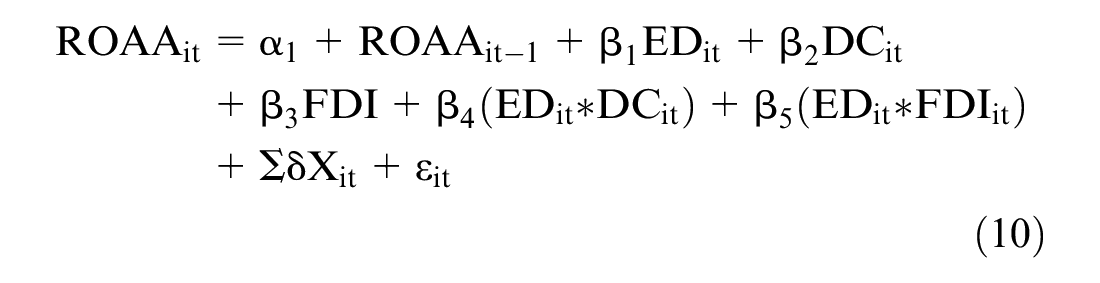
where ROAs_it and ROE_it are the dependent variables (proxies for bank profit/returns) for country i and time t, and α, β₁, β₂, β₃, and β₄ are the coefficients to be estimated. (ED_it*DC_it) is the product of ED and DC and therefore their interaction. Likewise, (ED_it*FDI_it) is the product of ED and FDI and therefore captures their interaction.

(Food-Xo_{it it}*DC_it) is the product of agriculture production and domestic credit and therefore captures their interaction. meanwhile, (Food-Xo_{it it}*FDI_it) is the product of agriculture production and FDI and therefore captures their interaction (Yusheng et al., 2021). These interaction models are specified based on other studies (Afonso & Blanco-Arana, 2022; Aguinis & Gottfredson, 2010; Jaccard et al., 2003).

Z-Score Metrics for Bank Risk and Stability: Measures for Robustness

The z-score can be defined as a data score’s (e.g., bank returns) number of standard deviations from the mean. The Altman z-score equation was specified to ensure the consistency of the bank stability outcomes (Altman et al., 2017; Chouhan et al., 2014). The z-score was used as a dependent variable in the model following the specification parameters used in Models (1) to (4):

$$\begin{array}{c}\multicolumn{1}{c}{\mathrm{Z}-\mathrm{scor}{\mathrm{e}}_{\mathrm{it}}={\mathrm{\alpha }}_1+\mathrm{Z}-\mathrm{scor}{\mathrm{e}}_{\mathrm{it}-1}+{\mathrm{\beta }}_1\mathrm{E}{\mathrm{D}}_{\mathrm{it}}+{\mathrm{\beta }}_2\mathrm{F}{\mathrm{D}}_{\mathrm{it}}}\\ \multicolumn{1}{c}{+{\mathrm{\beta }}_3\mathrm{FDI}+{\mathrm{\beta }}_4(\mathrm{E}{\mathrm{D}}_{\mathrm{it}}*\mathrm{F}{\mathrm{D}}_{\mathrm{it}})+\sum \mathrm{\delta }{X}_{\mathrm{it}}+{\mathrm{\epsilon }}_{\mathrm{it}}}\end{array}$$

(14)

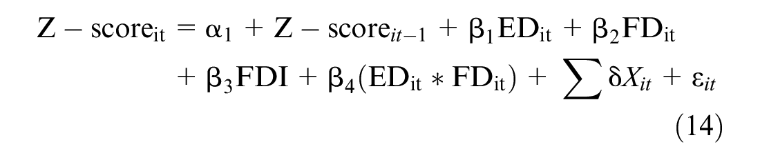
To evaluate the risks to bank stability, a volatility measurement was employed to assess the consistency of bank earnings during the entire study period. The formula to compute the z-score is: z-score = (ROA + ETA)/ (σ (ROA)) for asset earnings and z-score = (ROE + ETA)/ (σ (ROE)) for equity earnings, with ETA representing the equity-to-asset ratio and σ (ROA) and σ (ROE) representing the standard deviations for returns for assets and equity, respectively (M. Ali & Iness, 2020; Altman & Hotchkiss, 1993). The standard deviation for both types of earnings (ROA and ROE) was calculated for bank i in year t as in (Kasman & Kasman, 2016). The equations were specified as follows:

$$\mathrm{\sigma }(\mathrm{ROA}{)}_{i,t}=\sqrt{\frac{1}{T-1}{\left(\sum _{t=1}^{t-T}(\mathrm{RO}{A}_{i,t}-\frac{1}{T+1}\sum _{t=1}^{t-T}\mathrm{RO}{A}_{i,t})\right)}^2}$$

(15)

$$\mathrm{\sigma }(\mathrm{ROE}{)}_{i,t}=\sqrt{\frac{1}{T-1}{\left(\sum _{t=1}^{t-T}(\mathrm{RO}{E}_{i,t}-\frac{1}{T+1}\sum _{t=1}^{t-T}\mathrm{RO}{E}_{i,t})\right)}^2}$$

(16)

Data Source and Descriptive Statistics

Variables Descriptions and Sources

We collected data from two different sources: the macroeconomic variables from the World bank development indicators database (www.data.worldbank.org) and bank-specific variables from the Bank Focus database (www.moodysanalytics.com). This study used unbalanced panel data with N > T (where N was equal to 40 countries and T was 9 years). The data sample covers 40 countries with 350 active banks. We organized the downloaded ratios and treated them in MS Excel and then uploaded into Stata software (version 15). We run xtabond2, for the regression analysis for the two-step system GMM (Roodman, 2009). Table 1 lists the states across the three regions of SSA and the share of banks in each of the three regions out of the total number of banks. The ECOWAS has a highest number of states (15) and of banks (42.82%).

Table 1.

States and Bank Shares in SSA.

Primary region	Secondary region	No. of States	States	Bank share (%)
SSA	EAC	6	Burundi, Kenya, Tanzania, Rwanda, Uganda, and South Soudan	22.13
	ECOWAS	15	Benin, Burkina Faso, Cap Verdo, Ivory coast, Gambia, Ghana, Guinea, Guinea Bissau, Liberia, Mali, Niger, Nigeria, Sierra Leone, Senegal, and Togo	42.82
	SADC	16	Angola, Botswana, Comoros, Democratic Republic of Congo, Eswatini, Lesotho, Madagascar, Malawi, Mauritius, Mozambique, Namibia, Seychelles, South Africa, Tanzania, Zambia, and Zimbabwe	33.91
	Others	2	Ethiopia, Djibouti	1.15
	TOTAL	40		100.00

The most recent version of Bank Focus contained calculated bank ratios starting from 2011; our institutional time access was limited to 2019. The macroeconomic variables are as follows: ED represents economic development (Ductor & Grechyna, 2015; Yusheng et al., 2021). TGE represents total government expenses, which is a proxy for monetary supplier (Calderón & Liu, 2003). DC represents domestic credit given to the private sector by commercial banks (Afonso & Blanco-Arana, 2022; Mtar & Belazreg, 2021). FDI represents foreign direct investment cash inflow (Samour et al., 2022; Siddikee & Rahman, 2021). INFL is the inflation rate. Agro-production is proxied by food production and used to assess real edible food that contains nutrients, which is crucial for human health and life. It is used because agricultural products are the main contributor to African ED (Gollin, 2020; Suri & Udry, 2022).

The bank-specific variables included LLRs, which is the ratio of LLRs or provisions to gross loans, and NPLs, which represent the ratio of NPLs to gross loans. These two ratios represent the dependent variables as bank stability metrics. The returns ratios (ROA and ROE) represent the dependent variables for bank profitability. The TC ratio represents the bank’s total capital ratio and was included as a proxy to capture the effect of bank size. Macroeconomic and bank-specific variables were used as strong instrumentals to avoid biasness in the results (Burgess & Thompson, 2011). We use logarithm form to avoid inflated results.

Descriptive Statistics

In Table 2, the data of all the variables are standardized at3,480 observations. The standard deviation varies from 3.024 to 0.064. ED–DC has the highest standard deviation (4.292), because the ED of developing countries varies significantly across countries and differs from one country to another (e.g., Nigeria vs. Eritrea).

Table 2.

Descriptive Statistics.

Variable	Obs	Mean	Std. Dev.	Min	Max
Bank specific variables
Z_SCOROE	3,480	2.514	1.069	−1.410	13.661
Z_SCOROA	3,480	3.514	1.869	−1.819	13.661
ROAA	3,480	1.688	1.840	−5.077	6.599
ROAE	3,480	2.286	1.492	−3.353	8.449
NPL	3,480	3.318	0.217	3.027	3.612
LLR	3,480	2.395	0.666	1.211	3.941
DC (DOMECRE)	3,480	2.940	0.748	1.308	10.602
Macroeconomic Variables
ED (ECODEV)	3,480	2.082	3.024	−0.919	19.012
FDI (FODINV)	3,480	9.439	1.886	18.020	24.090
B-SIZE	3,480	2.628	0.107	2.425	2.753
TOTGOVEX	3,480	2.991	0.064	2.810	3.036
INFLAT	3,480	1.514	0.216	1.215	1.943
Food-Xo	3,480	1.081	0.640	−5.077	6.599
Interaction effects between independent variables
ED_DC	3,480	4.557	1.298	1.616	20.495
ED_FDI	3,480	22.187	4.292	3.452	40.863
Food_DC	3,480	4.646	1.46	1.677	6.11
Food_FDI	3,480	5.062	4.161	−9.18	11.439

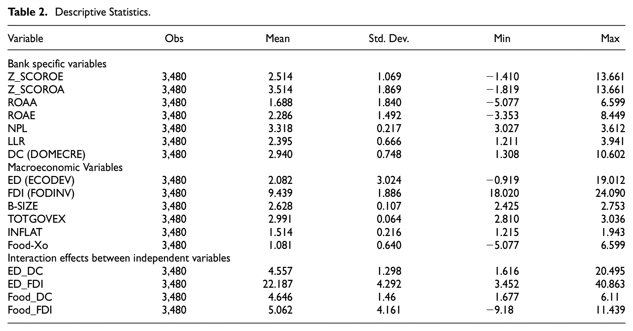
In contrast, TGE has the lowest standard deviation, which may be due to fixed government expenditures. The B-SIZE standard deviation is also very low because banks’ total capital ratios are mostly fixed at their beginning level. ED*FDI has the highest mean (22.184) and the highest maximum (40.868), which may imply that FDI plays an important role in ED in SSA.

Empirical Results and Discussion

The Effects of the Interactions Between ED, DC, and FDI on Bank Risk Alleviation

Table 3 displays the results for bank risk proxies (NPLs and LLRs a). The effect of DC on the NPLs is negative and statistically significant at a 1% significance level, ceteris paribus. Meanwhile, it is positive and statistically significant at a 1% significance level when DC influences the LLRs. ED negatively affects the risk factors: it reduces the NPLs (−1.018) at a 1% significance level but affects the LLRs positively (0.842) at a 5% significance level, ceteris paribus. Additionally, FDI affects the NPLs (−0.790) negatively, while the LLRs are affected positively at both 1% and 5% significance levels, ceteris paribus (Ma & Yao, 2022). Similarly, the effects of the ED– DC interaction reduce the NPLs (−1.873) at a 1% significance level, ceteris paribus (confirmation of H1a), while the same interaction positively affects the LLRs (1.620) at a 5% significance level, ceteris paribus; this confirms H1b (Mpofu & Nikolaidou, 2018). Similarly, the interactions between ED–FDI negatively influence the NPLs (−1.168) at a 1% significance level (Xie et al., 2022) and positively impact the LLRs (2.026) at a 1% significant level, ceteris paribus; this confirms H2a and H2b.

Table 3.

Two-Step System GMM Results (for Bank Stability Models Via Risk Factors).

Bank Risk: NPLs Models (Model 6)					Bank Risk: LLR (Model 7)
Models	GMM Results		2SLS Results		GMM Results		2SLS Results
Indep.Vars	Coefficient	Corr.Std. Error	Coefficient	Std. Error	Coefficient	Corr.Std.	Coefficient	Std. Error
NPLlag	−0.000 **	0.004	—	—	−0.127***	0.027	—	—
DC	−0.473***	0.052	−2.083***	9.768	1.011***	1.285	−2.039***	5.103
ED	−1.018***	1.058	−0.510**	1.180	−0.842*	−0.97	−0.605***	6.090
FDI	−0.790*	0.341	1.350**	7.620	1.785**	1.538	1.070**	4.370
DC_ED	−1.873***	1.085	−3.925***	6.652	1.620***	1.191	2.13***	3.418
FDI_ED	−1.168***	2.221	−1.598**	0.563	2.026***	1.192	0.896**	0.283
Bank-Size	1.140	0.018	−1.037**	0.810	0.023	0.087	−1.168*	0.549
TGE	0.209	1.107	−0.532	4.656	0.478***	0.276	−4.876	8.949
INFLAT	−1.040***	0.190	−0.233*	0.625	−0.317***	0.037	1.114**	0.333
Statistics	AR (1)	0.207	Darbin	0.000	AR (1)	0.428	Darbin	0.000
for	AR(2)	0.097	Hausman	0.000	AR(2)	0.116	Hausman	0.000
Models	Hansen	0.439	Sergan	0.965	Hansen	0.157	Sergan	0.965

***

, **, and * respectively indicate significance at the 1%, 5%, and 10% levels.

The overall confirmation of H1a, H1b, H2a, and H2b validates the general hypothesis (H3). Furthermore, the effects of ED–DC on NPLs and LLRs are higher than the factors’ (ED, DC, and FDI) individual effects; this proves that the interaction effects play a significant role in bank sustainability by reducing the bank riskiness (Ma & Yao, 2022). Figures 3, 4, 8, 9 support these results, and show the co-movements of these three interacting variables (ED, DC, and FDI); markedly, based on their co-movements similar since 1970.

Figure 8.

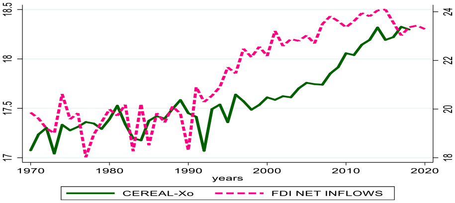
Evolution of cereal production and FDI net inflows

Figure 9.

Evolution of GDP growth and food production in SS Africa.

Furthermore, the second findings for robustness with 2SLS regressions are consistent with the GMM results. Therefore, the outcomes of both regression techniques exhibit convergence. Moreover, the consistency of the results is maintained when utilizing cereal production factors instead of food production, thereby demonstrating the reliability of our results.

Economic expectations support these results because, in normal conditions, the two variable groups (risk and profit proxy groups) seemed to react differently. The more the bank risk factors are reduced, the higher the bank returns are, and vice versa. NPLs act as a determinant for the default risk and for the whole banking system; however, they are driven by ED (Mpofu & Nikolaidou, 2018). This explains why ED’s interactions with DC and FDI greatly impact bank risk reduction while simultaneously increasing bank profitability. Moreover, if DC is developed, then it will increase ED, which sustains the banking sector through well-performing loans (Mpofu & Nikolaidou, 2018).

The Effects of the Interaction Between ED, FD, and FDI on Bank Returns

Table 4 displays the results of the profitability models using ROA and ROE as dependent variables. FD positively affects both ROA (0.59) and ROE (1.314), and ROA is statistically significant at a 1% significance level, ceteris paribus. The effect of ED on both ROA (0.830) and ROE (1.258) is also positive and statistically significant at a 1% significance level, ceteris paribus. However, the impact of FDI on ROA (−1.15) is negative and statistically insignificant, while its effect on ROE (0.832) is positive and statistically significant at a 5% significance level, ceteris paribus. Meanwhile, the interaction effects of DC–ED on ROA and ROE (1.314) are positive and statistically significant at a 1% significance level, ceteris paribus; this confirms H2a). The influence of FDI–ED on ROA is negative (0.960) but not significant, while its effect on ROE is positive and statistically significant at a 1% significance level, ceteris paribus; this confirms H2b).

Table 4.

Two-Step System GMM and 2SLS Results (for Bank Stability via Profit proxies).

Bank Profit: ROA Models (Model 10)					Bank Profit: ROE (Model 11)
Models	GMM Results		2SLS Results		GMM Results		2SLS Results
Indep.Vars	Coefficient	Corr.Std. Error	Coefficient	Std. Error	Coefficient	Corr.Std.	Coefficient	Std. Error
NPLlag	1 ***	0.000	—	—	0.302***	0.028	—	—
DC	0.59***	0.315	0.704**	0.044	1.314***	0.528	1.178***	2.121
ED	0.830***	1.150	1.584	0.998	1.258***	0.121	1.350***	2.90
FDI	−1.15	1.681	−0.327***	0.088	0.832**	1.291	−3.810***	1.830
DC_ED	1.25***	1.124	1.239**	1.017	1.391**	1.582	3.072***	0.399
FDI_ED	−0.960	0.570	2.251***	8.891	1.493***	0.140	−0.375***	0.30
Bank-SIZE	−0.205	0.153	0.527***	0.089	0.460	003	1.978**	0.192
TGE	−0.401	0.019	−0.396	3.079	0.644***	0.010	0.146	8.721
INFLAT	1.740***	1.408	−0.287***	0.077	0.031	0.275	2.275	0.154
Statistics	AR (1)	0.207	Darbin	0.000	AR (1)	0.428	Darbin	0.000
for	AR(2)	0.097	Hausman	0.000	AR(2)	0.116	Hausman	0.000
Models	Hansen	0.493	Sergan	0.176	Hansen	0.115	Sergan	0.353

***

, **, and *respectively indicate significance at the 1%, 5%, and 10% levels.

The results of the two-stage least square (2SLS) regression in the Tables 4 and 5 align with those of the generalized method of moments (GMM), thereby substantiating the positive and significant impacts of these interactions on the bank’s earnings. The consistency of the results is maintained when substituting the food production factor with the cereal production factor, indeed confirming the reliability of the findings.

Table 5.

System GMM Results for Bank Risk and Profitability (Interactions with Food-Xo).

Models	LLR (MODEL 8)		NPLs (MODEL 9)		ROA (MODEL12)		ROE(MODEL(13
Independent variables	Coef.	C.Std. Error	Coef.	C.StdError	Coef.	C.Std. Error	Coef.	C.StdError
Lag(−1)	−0.03***	0.015	−0.003***	0.015	0.255**	0.019	−0.293**	0.015
DC (DOMECRE)	−0.351*	0.182	0.470**	0.182	0.079**	0.129	1.090**	2.144
FOOD-Xo	0.420	0.234	−0.310**	0.004	0.608*	0.710	0.712**	0.474
FDI (FODINV)	1.285*	2.923	1.285**	2.923	0.907	−4.79	−0.050**	0.000
DC* FOOD-Xo	0.812**	0.070	−0.604**	0.434	1. 329***	0.843	2.407***	0.065
FDI*FOOD-Xo	2.601***	0.654	−1.266***	0.051	3.915***	1.000	4.060***	1.112
Bank-SIZE	0.028*	0.007	−0.012*	0.007	1.102	0.743	0.604**	3.062
TGE	1.020	1.916	1.020**	1.916	−0.154	0.060	−1.000	2.905
INFLAT	−0.047**	0.021	0.047	0.021	−0.886*	0.165	−1.652	3.798
Statistics	AR (1)	0.337	AR (1)	0.712	AR (1)	0.135	AR(1)	0.135
For	AR(2)	0.812	AR(2)	0.973	AR(2)	0.817	AR(2)	0.798
Models	Hansen	0.152	Hansen	0.479	Hansen	0.196	Hansen	0.235

***

, **, and *respectively indicate significance at the 1%, 5%, and 10% levels.

The confirmation of H2a and H2b validate H2 related to profitability. Furthermore, the ED–FD effects on ROA and ROE are higher than DC and FDI’s individual effects, but not ED’s individual effects; this confirms H3. These results are further validated by the trends evident in Figures 1, 3, 10, which show that the co-movement of these three main variables have increased since 1970. Collectively, these findings confirm the complementarity between these three macroeconomic factors. The proxies for bank profitability generally moved in the same direction (Figures 6 and 11), while the proxies for bank riskiness generally moved in opposite directions (Figures 7 and 12). The increase in LLRs indicates that NPLs decreased and could provide a better profit from the net margin for the bank; this is why the LLRs moved in step with the ROE.

Figure 10.

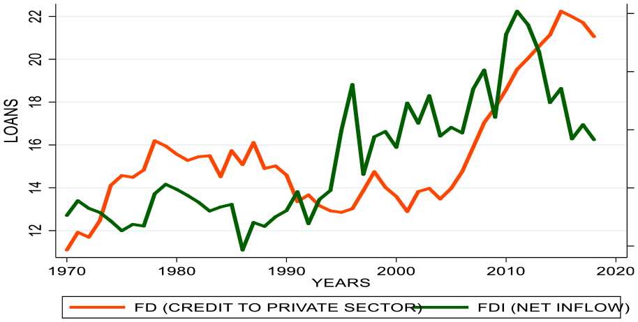
Evolution in scissors effects: FDI and domestic credit growth.

Figure 11.

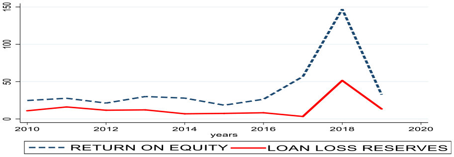
Cointegration between LLRs and ROE.

Figure 12.

Inverse moves between Non-Performing Loans and Return on Equity

The Effects of the Interactions Between Food Production, FD, and FDI on Bank Sustainability Through Risk and Profit Shocks

Another interaction effects group was introduced using the agricultural production factor (Food-Xo), as it is the main contributor to African ED growth (Suri & Udry, 2022). Table 5 presents the results for its interactions using GMM methods with Models 8, 9, 12, and 13. ED and Food-Xo impact bank sustainability significantly by reducing risk and increasing profit, but their interactions effects are significantly higher than their individual effects. These results indeed confirm H4 and H5.

Discussion

The study’s findings indicate that the correlation between Food-Xo and DC has a significant and positive effect on all bank profit indicators at a 1% level of significance. The interaction effects exhibit statistical significance at the 5% and 10% levels, which is consistent with the significance levels observed for the individual impacts of Food-Xo and DC on bank profits.

Thus, the interaction effect has a positive and stronger impact on bank profit than the individual factors. These results confirm H5. Similarly, the interactions between Food-Xo and FDI on bank profit have a stronger and more positive impact on bank profit than the individual factors. The effects of these interactions on bank risk were negative and more significant (at a 1% level) than the individual effects (at a 10% level). In sum, the interactions negatively affect bank risk proxies and positively affect bank profit proxies. The inferences of these opposite effects are meaningful for both bank risk and bank profits.

Thus, it can be inferred that the impact of the interaction effect on bank profit is more significant compared to that of the individual factors. These revealed findings provide support for Hypothesis 5. Similarly, the interactions between Food-Xo and FDI on bank profit exhibit a more pronounced and positively influence on bank profit as compared to their individual effects. The impact of the above interactions on bank risk is negative and statistically more significant (at a 1% level) compared to that of individual factors (at a 10% level). To summarize, these interactions have an adverse impact on the risk indicators of banks while having a favorable effect on their profitability indicators. The implications of these contrasting impacts hold significance for both the risk and profitability of banks, for both GMM as well as 2SLS estimates.

Three findings are important in regards to bank risk alleviation via NPLs and LLR: Firstly, the interactions between both ED and Food-Xo with the factors of FD (DC and FDI) affect negatively NPLs. These results converge with other findings (Ma & Yao, 2022). These effects imply that these interactions reduce bank risk by decreasing NPLs. The stronger these interactions, the more they reduce bank risk and strengthen bank stability. These findings align with economic expectations: increases in these interactions with FD factors increase real production and ED (Purewal & Haini, 2022), which ultimately sustains the banking system by reducing bank risk (Ma & Yao, 2022).

Secondly, in contrast, the interactions positively influence bank risk through LLRs. This implies that increases in the strength of the interactions between these factors will increase bank reserves and liquidity (S. Ali et al., 2022), which will in turn improve bank security and stability (F. F. Abbas & Ali, 2022). These findings are supported by the fact that bank liquidity ratios are the main pillars that prevent banks from being ruined, as required by the Basel committee for bank settlement on liquidity requirement ratios (Le et al., 2023; Obadire et al., 2022). This explains why banks care the most about their liquidity ratios (S. Ali et al., 2022).

Thirdly, these findings are further confirmed in two different ways: (a) they converge well with the previous findings on bank risk regarding NPLs. In normal times, when NPLs decrease (and thus ROE increases), LLRs increase because banks do not use the loan loss reserves to cover loan losses (loans perform well and positively influence bank returns); the co-movement of the Figure 11 confirms these results. Furthermore, the Figure 13 illustrates the same meaning. (b) the two figures generated for these three variables confirm these results by showing the cointegrated movements of ROE and LLRs (see Figures 11 and 13) and the inverse movements of ROE and NPLs (see Figures 12 and 14).

Figure 13.

Ratio of loan loss reserves on non-performing loans and credit trends.

Figure 14.

Scissors movements between non-performing loans and bank liquidity ratio.

Concerning bank stability via increase in ROA and ROE, the interactions between FD factors and Food-Xo on the one side and FD factors and the ED on the other side, influence both bank profit proxies (ROE and ROA): the positive effects of the interactioneffects on bank returns imply that the stronger the interactions, the more the bank benefits (Joaqui-Barandica et al., 2022). These findings also align with economic expectations: when an increase in the interaction between ED and Food-Xo interacts with increases in the factors of FD, economic expansion generally occurs (Purewal & Haini, 2022). Bank credit is the fuel for both agricultural production and economic expansion (Ngong, Onyejiaku et al., 2022), and in doing so, bank credit helps in fulfilling the social reasonability of financial institutions (Jiang & Kim, 2020). Under such circumstances, a borrower can conveniently reimburse the interest and principal of their loan, thereby promoting economic, and bank performance. The loans (DC) performance sustains both bank and ED performance. When loans perform well, bank returns increase (i.e., the bank is paid the interest on the loan), and bank can reinvest again by offering more credits and continue cyclically to generate more profit. Hence, we can confirm that these interactions increase bank sustainability through their positive effects on bank returns as long as they sustain loan performance. Otherwise, if loans do not perform well, they can cause stress in the banking system and generate crisis as in 2008 USA Credit bubbles (Huang et al., 2019; Ivanov et al., 2016; Luchtenberg & Vu, 2015; Pattnaik et al., 2020).

Robustness Checks

Robustness Results1 for Bank Risk With z-Score for the Entire Dataset

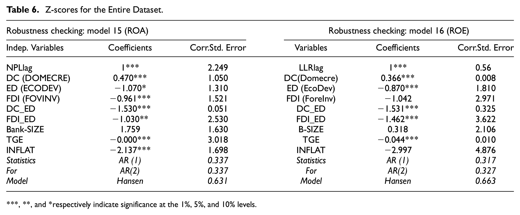
Table 6 reports the results for the z-score of the entire dataset for all countries. These interaction effects negatively affect the two z-scores (−1.530, −1.030 for ROA and −1.531, −1.462 for ROE) and are statistically significant at a 1% level. Moreover, they have a stronger impact than the individual effects of each variable. The impact of the ED–DC interaction is stronger that of the ED–FDI interaction. These results crucially imply that these variables significantly affect bank risk and stability by considerably reducing the z-score—the lower the z-score, the better bank stability (M. Ali & Iness, 2020; Kasman & Kasman, 2016). These findings evidence the robustness of the results obtained in Tables 3 to 5 and confirm H3 and H5.

Table 6.

Z-scores for the Entire Dataset.

Robustness checking: model 15 (ROA)			Robustness checking: model 16 (ROE)
Indep. Variables	Coefficients	Corr.Std. Error	Variables	Coefficients	Corr.Std. Error
NPLlag	1***	2.249	LLRlag	1***	0.56
DC (DOMECRE)	0.470***	1.050	DC(Domecre)	0.366***	0.008
ED (ECODEV)	−1.070*	1.310	ED (EcoDev)	−0.870***	1.810
FDI (FOVINV)	−0.961***	1.521	FDI (ForeInv)	−1.042	2.971
DC_ED	−1.530***	0.051	DC_ED	−1.531***	0.325
FDI_ED	−1.030**	2.530	FDI_ED	−1.462***	3.622
Bank-SIZE	1.759	1.630	B-SIZE	0.318	2.106
TGE	−0.000***	3.018	TGE	−0.044***	0.010
INFLAT	−2.137***	1.698	INFLAT	−2.997	4.876
Statistics	AR (1)	0.337	Statistics	AR (1)	0.317
For	AR(2)	0.337	For	AR(2)	0.327
Model	Hansen	0.631	Model	Hansen	0.663

***

, **, and *respectively indicate significance at the 1%, 5%, and 10% levels.

Robustness Results2 With Two-Least Square Regressions

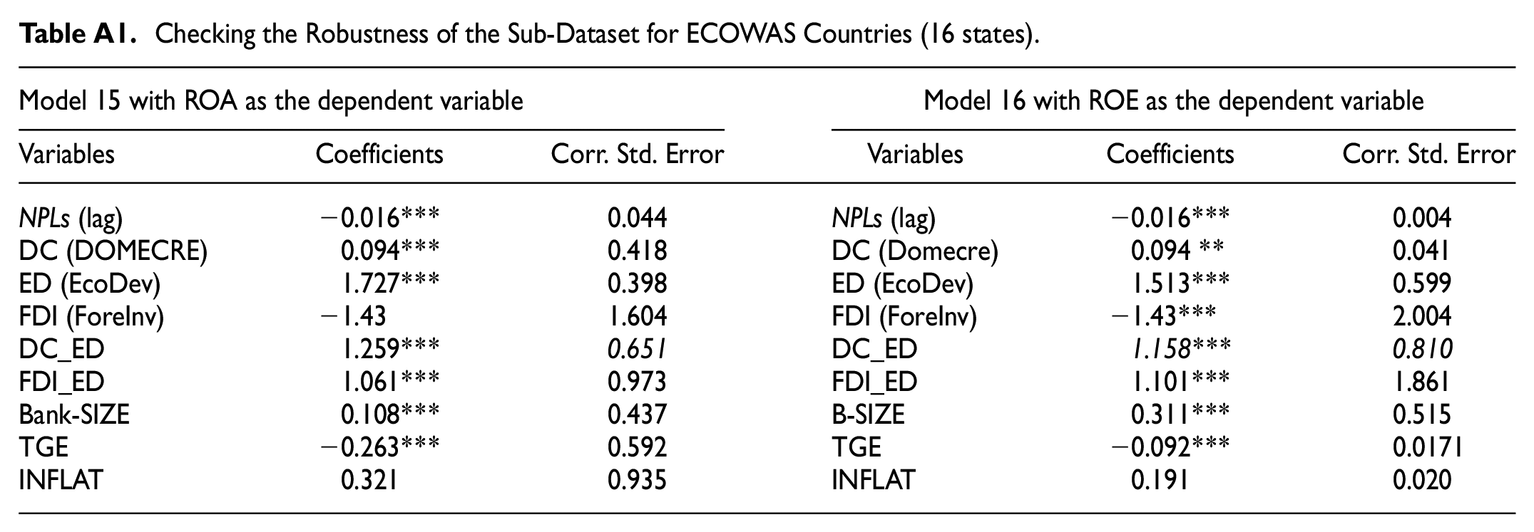
The outcomes of 2SLS regressions using the same model specifications and data set are presented in Table 7. These results confirm those derived by regressing the GMM model at both the SSA and sub-regional levels. The Table 1 in the Appendix A displays the sub-regional results. All of these results indicate that their interactions have substantial negative effects on both risk and positive impacts on profit. Moreover, these interaction effects are higher and statistically significant than their individual effects. In addition, these results are consistent when cereal production factor substitutes Food-Xo in the regression.

Table 7.

2SLS Regression Results for both Bank Risk and Profit (Interactions with Food-Xo).

Models	LLR (Model 8)		NPLs (Model 9)		ROA (Model 12)		ROE (Model13)
Independent variables	Coef.	Std. Error	Coef.	Std. Error	Coef.	Std. Error	Coef.	Std. Error
DC (DOMECRE)	0.107**	0.036	0.106***	0.039	−8.288***	2.765	1.488**	0.707
FOOD-Xo	−3.512*	1.982	−5.811**	2.386	−1.068***	1.067	0.113	0.082
FDI (FODINV)	−2.680	1.800	−1.810	2.210	−1.140***	4.190	−1.760*	9.700
DC* FOOD-Xo	−3.120***	1.048	3.063***	1.127	1.606***	0.026	0.714**	0.006
FDI*FOOD-Xo	3.371**	1.881	−2.411**	2.230	2.791**	4.030	1.881**	1.041
Bank-SIZE	−0.112*	0.067	0.154	0.095	0.054	1.499	−0.022	0.212
TGE	0.012*	0.007	0.025***	0.008	−0.204	0.112	4.361	7.105
INFLAT	−0.007	0.005	−0.003	0.005	2.798	1.172	−0.650	0.403
Test type	statistic	P.V	statistic	P.V	statistic	P.V	statistic	P.V
Durbin	5.216	0.022	3.205	0.073	16.119	0.000	24.170	0.000
Hausman	5.187	0.023	3.178	0.075	16.265	0.000	24.551	0.000
Sergan	0.787	0.374	1.017	0.313	0.251	0.615	2.739	0.097
Basman	0.779	0.377	1.006	0.315	0.248	0.618	2.718	0.099

***

, **, and *respectively indicate significance at the 1%, 5%, and 10% levels.

Conclusion

Based on our findings, we imply that the interactions between the three macroeconomic factors, namely agriculture production, economic development, and financial development factors (represented by FDI and DC), improve bank sustainability by significantly reducing NPLs and inversely increasing LLRs on the one hand. On the other hand, increase bank returns via a rise in ROE and ROA and significantly improve bank performance. The outcomes of various regressions validate our hypotheses and converge with different regression techniques at the SSA level and sub-regional levels.

The confirmation of H1a and H1b provides support for the hypothesis H1. The confirmation of the hypotheses H2a and H2b serves to validate hypothesis H2. Furthermore, the verification of the hypotheses H1 and H2 substantiate hypothesis H3. However, the analysis of the results presented in Table 5 (with GMM and 2SLS estimates) confirm all the hypotheses from H1 to H5. Those gradual validations of these hypotheses (through their related sub-hypothesis) answer our research questions stated toward the end of the Introduction part. Ultimately, our findings comply with our main objectives.

Consequently, we conclude that the interaction effects between the three macroeconomic factors are complementary and contribute significantly to the sustainability of African banks. This is evidenced by the fact that the combined effects of these factors are considerably greater than their individual effects in sustaining the banking system in Africa.

The Recommendations

• The findings indicate that the interactions have an adverse impact on bank risk, therefore, study recommends that intermediary institutions in Africa should allocate capital directly to the agriculture sector to foster economic development and mitigate bank risk by minimizing non-performing loans.

• Study recommends that banks in SSA nations should act more aggressively and take on more risk when providing credit to farmers, which would boost their earnings on both returns

• Study recommends that central banks in Sub-Saharan African (SSA) nations implement updated regulations relating to agricultural financing, with the aim of incentivizing commercial banks to incorporate a mandatory minimum allocation of agricultural credit within their overall credit portfolios.

• Study recommends that governments provide collateral in the form of insurance schemes for smallholder farmers, given that numerous African households rely on traditional farming methods.