Sage Journals: Discover world-class research

Abstract

To better understand the actual rating variables that affects Auto insurance Policyholders’ premium, this paper attempts to provide empirical evidence to justify which ones are significant and needed to be considered by insurers by adopting the autoregressive distributed lag (ARDL) model. In satisfying all the conditions for ARDL application, unit root, Heteroskedasticity, normality, dynamic stability and serial correlation tests were conducted. We estimate the effects of each rating variable on Premium taking into consideration whether the policy of the insured is Third-Party or Comprehensive. These rating variables in the ARDL model serves as the independent variables that establishes the short and long-run relationships between them and the Premium as the dependent variable. The results suggest that not all the classical rating variables used in the market significantly impact Premium. Whiles, to some extent, we found a varying degree of variables impact on Premium depending on the insurance type, the autos cubic capacity, which plays a cogent role on the basic Premium in Ghana, is insignificant. Also, policyholders’ age characteristics are statistically significant but are excluded in the premium calculations. Thus, this paper shows the need to consider all the other possible rating variables, including policyholders’ age into the Ghanaian insurance pricing system, whiles autos cubic capacity considering the weight it put on the basic Premium should be re-examined. This would help to obtain a financially balanced and optimal pricing system for policyholders.

Keywords

long-run equilibrium classical Premium variables Ghana auto insurance market optimal pricing system insurance policyholders policyholders premium

Introduction

Automobile insurance, particularly the third-party (TP) category, is mandatory in most countries (Aeron-Thomas, 2002; Bülbül & Baykal, 2016; Isotupa et al., 2019; Lemaire, 1998). Automobile use has embedded morbidity and mortality risk, as well as loss through theft and fire in several countries (Lemaire, 2004), and thus its associated insurance was developed to handle the potential loss (Boucher et al., 2009; Frangos & Vrontos, 2001). Automobile insurance was introduce to safeguard policyholders from potentially enormous financial losses as well as losses to third parties. However, the premium, which is computed based on the policyholder’s risk, can influence the decision to purchase a policy (Alhassan, 2016; Alhassan et al., 2015; Alhassan & Biekpe, 2016a; Azaare et al., 2021; Bülbül & Baykal, 2016; Isotupa et al., 2019). Majority of studies look at premium estimates from a traditional perspective on the basis of claims frequency and severity from policyholders’ (Azaare et al., 2022; Deniut et al., 2007). From both a priori and a posteriori point of view, the frequency and severity of policyholder claims have been the major dependent variables in rate-making models. In the priori and posteriori structures of the bonus-malus system, some attributes of the policyholder and the vehicle are considered regressors. Classical variables such as the driver’s age, experience, career, marital status, gender, and the age of the vehicle, cubic capacity, mileage, garage location, and so on have been used in the priori premium determination setup (Jacob & Wu, 2020; Bolanc’e et al., 2007; Bülbül & Baykal, 2016). Nonetheless, the literature is not loud on the individual impacts of these classical variables on policyholders’ final premium, especially in the Ghanaian market (Azaare et al., 2021).

Furthermore, articles in the literature look at policyholders premiums by concentrating specifically on their driving patterns based on vehicle usage. As a result, premiums might be computed by relying on policyholders’ yearly distance traveled (Edlin, 2004; Ferreira & Minikel, 2012). In addition, the pricing system takes into account policyholders’ driving speed records, the most frequently plied roads, the type of such roads, and the time of day they are mostly on the roads (Langford et al., 2008; Litman, 2005; Paefgen et al., 2013, 2014; Sivak et al., 2007). According to Ayuso et al. (2014), “policies with these elements are mostly targeted at young drivers, but yet, there is a report on significant differences between novice and experienced young drivers, indicating a heterogeneous risk group among young policyholders.” Thus, insurers using policyholders age variable could lead to lower premium because older and experience drivers posed lower accident risk (Ayuso et al., 2014; Azaare et al., 2021). There are a number of interesting results when it comes to insurance variables that predict premiums. For instance, Boucher et al. (2013), as well as Litman (2005) and Langford et al. (2008) emphasized that the association between drivers’ number of claims and his distance driven may not be linear. Furthermore, the gender gap was linked to the frequency of vehicle use by Ayuso et al. (2016). While gender is important in explaining the time to the first accident, the authors argue that it is no longer necessary when the average distance traveled per day can be captured by telematics in the model to provide ample information on driving habits.

Surprisingly, despite all of the variables used by insurers in premium calculations, the Ghanaian auto insurance market based solely on vehicle age, cubic capacity, type of use for third-party policies, and inclusion of the vehicle’s sum in the comprehensive (C) premium case (Awunyo-Vitor, 2012; Ghana National Insurance Commission [NIC], 2015; Laryea, 2016), which this study discovers that not all of these variables are significant. The pricing model used by the market does not also capture any characteristics of the insured driver or the policyholder involved but relies on only the limited classical variables of the insured auto, leaving a mixed feeling from policyholders on variables considered because of the high nature of premiums (Azaare et al., 2021). According to the Ghana National Insurance Commission’s (NIC, 2015) pricing system, vehicles with fewer than 5 years of age are not charged age loading, but those with 5 to 10 and more than 10 years are paid 5% and 7.5% of the basic premium as age loadings, respectively. On the other hand, policyholders pay 5% and 10% of the basic premium for autos with a cubic capacity (CC) of 1601 to 2000 and >2000, respectively. Furthermore, in Ghana, the seating capacity of an insured vehicle plays a significant role in determining the final premium. “Except for the linear association between auto mass and accident severity, there is no sufficient evidence in the literature to support its inclusion” (Azaare et al., 2021).The standard number of seats included in the flat-rate system for both third-party and comprehensive insurance is five. In this situation, each vehicle with more than five seats pays 5 and 8 Ghana cedis per seat for private and commercial use, respectively (Azaare et al., 2021; Ghana National Insurance Commission [NIC], 2015).

Interestingly, extensive research conducted by Ayuso et al. (2017) indicates an insignificant relationship between insured auto age and accident or claims patterns, even in the telematics information model. Following Ayuso et al. (2017), we assume that since higher claims always lead to higher premiums, see Lemaire (1995), Mert and Saykan (2005), Denuit et al. (2009), and Sarabia et al. (2004), then Ayuso et al. (2017) findings implies an insignificant relationship between premium and auto age. Additionally, Boucher et al. (2013) postulates a non-proportional relationship between vehicle mileage/cubic capacity and claims occurrence. Beside, certain characteristics of the insured driver/policyholder, for examples the age, can never be underestimated in the quest for fair premiums since there is a distinctive heterogeneity among young and old drivers (McKnight & McKnight, 2003; Nicoletta, 2002). Thus, policyholders’ age is proportional to accident frequency and severity; older and experienced drivers have low accidents risk (Kelly & Nielson, 2006). Nonetheless, this risk variable is conspicuously missing from the pricing system used by the Ghanaian auto insurance market. This leads to the question: is the Ghanaian auto insurance market using the right rating variables that significantly have impact to justify high nature of policyholders premium? Hence, using the autoregressive distributed lag (ARDL) model, this study seeks to present empirical evidence to support which variables are significant and ought to be considered by insurers in order to better understand the actual rating variables that affect Policyholders premium. After thorough study, the data on the market met the requirements for ARDL, with no variable being I(2). “The ARDL model has a number of advantages/benefits over competing econometric models, including the fact that the dependent variable is explained not only by the independent variable(s), but also by its lag” (Bahmani-Oskooee & Brooks, 2003; Narayan, 2005; Pesaran et al., 2001; Phillips & Perron, 1988). “Endogeneity is less of an issue in the ARDL technique since it is free of residual correlation because each of the underlying variables stands as a standalone equation (i.e., all variables are assumed endogenous)” (Emeka & Aham, 2016). The ARDL approach can distinguish between dependent and explanatory variables, allowing us to assess the reference model. That is, the ARDL method presupposes that the dependent variable and exogenous variables have just one reduced form equation relationship (Pesaran et al., 2001). ARDL model can identify cointegrating vectors when there are several cointegrating vectors. The Error Correction Model (ECM) can be created from the ARDL model using a simple linear transformation, which integrates short run adjustments with long run equilibrium without destroying long run information. The ECM model’s lags are large enough to represent the data creation process in general to specialist modeling frameworks.

This model has been considered extensively in the literature. See, for example, Gouri’eroux and Jasiak (2004) who applied the autoregressive model to count for serial dependence in the count process.

Moreover, in the literature is level and long-run relationships determination through bound testing by Alhassan and Fiador (2014), Bahmani-Oskooee and Brooks (2003), Emeka and Aham (2016), Kaodui et al. (2020), Narayan (2005), Osuagwu (2020), Pesaran et al. (2001), and Phillips and Perron (1988). The ARDL model was used by Alhassan and Fiador (2014) to establish a long-run link between insurance company penetration in Ghana and economic growth by using the Pesaran et al. (2001) bound testing approach. Also in recent times, liquidity and firms viability nexus (Kaodui et al., 2020), output of manufacturing firms and agriculture long-run relationship (Osuagwu, 2020) are established. In addressing the gap as mentioned above in the literature, we present the first study analyzing the effects of rating variables on Premium using data from the Ghanaian auto insurance market in ARDL model.

“The Ghanaian auto insurance market is one of the largest in West African and, therefore, for many industry players, the most important sales market for their insurance policies” (Azaare et al., 2021). The historical backdrop of the insurance business in Ghana traces all the way back to the 1920s. The Guardian Royal Exchange Assurance Ghana Ltd was the first insurance company to start operation in the then Gold Coast in 1924 (Amoah & Nkrumah-Arkoh, 2009). From the year 1924 till date, the Ghanaian economy has been experiencing unprecedented penetration of insurance companies from both local and foreign front. The number of insurance businesses permitted to operate in the country increased to 53 at the end of 2018, according to the NIC annual report. A breakdown of the organizations shows that 17 are into life guaranteeing and 22 non-life. The statistics shows that 29 of these companies operate non-life (mostly auto) business whiles the remaining 24 do life business. Additionally, there are 82 insurance broking companies, three loss adjusting firms, four reinsurance brokers, and four reinsurance companies (Ghana National Insurance Commission [NIC], 2018). “The insurance business in Ghana is regulated by the National Insurance Commission (NIC), which has the object of guaranteeing successful organization, oversight, guideline, and control the matter of insurance in Ghana” (Duodu & Amankwah, 2011).

We had exclusive access to one of Ghana’s top insurance companies’ data sets in the sector of auto insurance. This study provides to the literature a better understanding of both long and short-run relationships that characterizes policyholder’s risk (rating factors) and their insurance cost (premium). Our results show that some of the rating factors, for example, cubic capacity of the auto, claims, and seating number for the comprehensive policy has an insignificant relationship with premium whiles there is the need for policyholders age inclusion into the pricing system particularly in the comprehensive policies because of its significance.

The contribution of this paper is to help insurers and government policy makers addressed concerns by policyholders on significant premium determinants for a fair pricing system by understanding the limitations and or opportunities involved in incorporating all other factors involved in auto insurance. According to studies, acquiring new policyholders costs five times more than keeping existing ones (Ampaw et al., 2019; Bhattacherjee, 2001; Chen & Myagmarsuren, 2011). As a result, the findings of this paper will serve as a forerunner and policy guide for insurance industry players in developing fair pricing systems by considering only rating factors that have a significant impact on premiums in order to improve policyholders’ retention rates with their various insurers. In addition, the paper aims to generate conversation topics that will elicit interest and debate on all possible premium determinants in the context of vehicle insurance in general. Although the study focuses on Ghana, the similarities in terms of factors considered by insurers when calculating auto insurance premiums in the sub-region and globally make our findings transportable.

The rest of the paper is organized as follows: Section 2 explains the materials and methods used for the study. In Section 3, we analyze and present the results. Finally, in Section 4, we discuss the findings and conclude.

Materials and Methods

In this section, the data, variables under consideration, and methods used to obtain desired results are discussed.

Data

Table 1 shows risk exposure and premium payment information for (N = 23,434) automobile insurance subscribers collected from a major Ghanaian insurance firm throughout 2018. The sample includes drivers who underwrote both third-party and comprehensive insurance policies. In the entire sample, n = 3,731 (15.9%) drivers had recorded claims, with a mean age of 48 years for both comprehensive (C) and third-party (TP), whereas the whole portfolio and those with no reported claims had a mean age of 49 years. We divided the data into two categories: TP n = 1940 (52.0%) and comprehensive n = 1791 (48.0%), with each category analyzed independently due to explanatory variable differences. For instance, with a comprehensive policy, we have the insured auto value, which is not required in a third-party policy. The descriptive statistics in Table 1 shed more light on the differences between policyholders who have reported claims and those who haven’t, as well as those who have comprehensive and third-party policies. The insured vehicle’s features are likewise shown in Table 1. Table 2 also shows the variables that were used in the model. The explanatory variables in our model are classical premium variables that are found in market data, such as policyholder age, insured vehicle age, cubic capacity, claims size, and vehicle seating capacity (Awunyo-Vitor, 2012; Azaare et al., 2021; Ghana National Insurance Commission [NIC], 2015; Laryea, 2016).

Table 1.

Claims and Variable Categories Descriptive Statistics (Quantitative Variables).

X1 (Premium)	Premium paid by the policyholder to the insurer in Ghana cedi
X2 (Sum insured)	The value of the insured vehicle for comprehensive policies in Ghana cedi
X3 (Vehicle age)	The age of the insured vehicle in years
X4 (Seat)	The number of seating capacity of the insured vehicle
X5 (Claims)	Claims reported/paid to the policyholder in Ghana cedi by the insurer
X6 (Cubic capacity)	The cubic capacity or the horsepower of the insured vehicle
X7 (Policyholder age)	The age of the policyholder or the driver in years

Table 2.

Description of the Variables.

Variable	Total sample(N = 23,434)		Policies with no claimsN = 19703 (84.1%)		Policies with claimsN = 3731 (15.9%)		Comprehensive policiesfrom claims N = 1791 (48.0%)		Third-party policies from claims N = 1940 (52.0%)
Variable	Mean Std		Mean Std		Mean Std		Mean Std		Mean Std
×1	854	1,915	813	1,815	842	1,666	1,512	2,216	224	105
×2	27,784	-	26,270	58,505	29,648	61,105	66,747	222,965	-	-
×3	11	7	11	7	12	6	9	6	14	24
×4	6	5	6	33	5	4	5	3	7	45
×5	1,522	9,799	-	-	9,547	22,941	10,659	27,203	8,481	18,043
×6	2,456	1,077	2,461	1,078	2,442	1,068	2,466	1,097	2,419	1,040
×7	49	16	49	16	48	16	48	16	48	16

The Autoregressive Distributed Lag Model

The autoregressive distributed lag model (ARDL) is an infinite lag distributed econometric model that is used to deduce long-run associations from short-run situations. The ARDL model has a number of advantages/benefits over competing econometric models, including the fact that the dependent variable is explained not only by the independent variable(s), but also by its lag (Bahmani-Oskooee & Brooks, 2003; Narayan, 2005; Pesaran et al., 2001; Phillips & Perron, 1988). In order to investigate the existence of a relationship between premium and our explanatory variables, we formulate our ARDL in broad terms as follows:

\begin{matrix} Δ Y_{t} = β_{0} + \sum_{i = 1}^{n} β_{i} Δ y_{t - i} + \sum_{i = 1}^{n} ϖ_{i} Δ X_{t - i} + δ_{1} y_{t - 1} \\ + δ_{2} X_{t - 1} + μ_{t} \end{matrix}

(1)

From (1), we expand it as;

\begin{matrix} Δ Y_{t} = β_{0} + \sum_{i = 1}^{n} β_{i} Δ y_{t - i} + \sum_{i = 1}^{n} ϖ_{1} X_{2 t - i} + . . . + \\ \sum_{i = 1}^{n} ϖ_{6} X_{6 t - i} + δ_{1 yt - 1} + δ_{2} X_{2 t - 1 + . . . +} δ_{7} X_{6 t - 1} + μ_{t} \end{matrix}

(2)

Where $β_{i}$ and $ϖ_{i}$ are the short-run coefficients for Premium and the independent variables approaching equilibrium, $δ_{1}$ , $δ_{2}$ , … $δ_{7}$ are the autoregressive distributed lag long-run coefficients for Premium and the six independent variables, and $μ_{t}$ is the model’s white noise. For both the short-run and long-run coefficients, we show the difference between the change in Premium (Y) on the left side and its own lag components in the right side (y) in (1) and (2). For the comprehensive policy, the independent variables are also indicated by $X_{2}, X_{3} . . . X_{7}$ and is reduced to five in the third-party situation. In addition, $n$ is the optimal model lags in both equations which is one for comprehensive and three for third-party. The lag residuals (LR) and the model for the long run (LRM) association are defined as follows:

\begin{matrix} LR = y_{t} = β_{0} + β_{1} X_{t} . . . β_{n} X_{t} + ε_{t} \\ LR = Z_{t - 1} = y_{t - 1} - b_{0} - b_{1} X_{t - 1} \end{matrix}

(3)

In this approach, the error correction term is substituted with $y_{t - 1}$ and $X_{t - 1}$ in (3). We replaced the long run term ( $δ_{1} y_{t - 1} + δ_{2} {X_{2}}_{t - 1} . . . + δ_{7} X_{7 - 1}$ ) with its residual to estimate the error correction model (ECM). Notwithstanding, the lag residual exists as $Z_{t - 1} = y_{t - 1} - b_{0} - b_{1} X_{t - 1}$ . As a result, the same lagged levels as in the ECM are included in this ARDL model, but their coefficients are not restricted. As a result, our ARDL model is a type of unrestricted ECM, suggesting that we have specified all of our long-run relationship variables ( $X_{it - 1}$ ). The speed with which the model adjusts from short-run to long-run equilibrium is estimated as

σ = 1 - \sum_{i = 1}^{n} β_{i}

(4)

with estimated long-run coefficients given by;

\overset{Λ}{θ_{i}} = \frac{\sum_{i = 1}^{n} {\overset{Λ}{β}}_{i}}{1 - (\sum_{i = 1}^{n} \overset{Λ}{σ_{i}})}

(5)

It’s worth noting that Y(y) is the X1 reading from our Table 2 variables.

There are various conditions that must be met in order to determine the appropriateness of an ARDL application, which, as previously said, characterize the data under consideration. These conditions have also received a lot of attention in the literature. For example, unit root testing and other conditions such as heteroskedasticity, normality, dynamic stability, serial correlation test, and others, used by Dickey and Fuller (1979, 1981), Engle and Granger (1987), Granger (1983), and Granger and Lin (1995), in applying ARDL model to identify relationships among I (0) or I (1) dependent and independent variables.

Testing Long-Run Relationship Presence

With the help of the EViews version 10 software used in this paper, we established the existence of long-run relationships between premium and the independent variables by adopting the Pesaran et al. (2001) bound testing. In this case, we use the F-statistics to test depending on the number of lags the individual or joint null hypothesis as follows;

$H_{0} : σ_{1} = σ_{2} = . . . = 0$ , $H_{1} : σ_{1} \neq σ_{2} \neq . . . \neq 0$ .

The decision here is that there is statistical evidence to support the existence of a long-run relationship if the null hypothesis is rejected (F- value >Pesaran upper critical bound value at 0.05 level).

Analysis and Results

Ascertaining Data Conformity with ARDL Conditions and Optimal Lag Selection

To choose the best model to establish the underlying long-run relationship, it was important to use proper model order criteria selection in determining the optimum lag. This was needful in obtaining standard normal error terms that satisfy normality, free from autocorrelation and heteroskedasticity. The appropriate model order selection criteria employed in this study are the Akaike Information Criterion (AIC) and the Schwarz Information Criterion (SIC). In concluding as to which lag is appropriate for the long-run model, various lags of the variables were estimated, compared, and the lag length with the smallest AIC and SIC was considered the most optimal. As shown in Table 3, lag 1 and lag 3 are optimal for comprehensive and third-party, respectively. Hence, we developed our original ARDL models for both categories based on their optimal lags as shown in Tables 4 and 5.

Table 3.

Statistics for Selecting Model Optimal Lag.

Comprehensive	t-Statistics	p-Value
Null hypothesis: The variables have unit root
Augmented Dickey-Fuller test Statistic	−40.35237	.0000
Test critical values (%)
1%	−3.433801
5%	−2.862951
10%	−2.567568
Third party
Null hypothesis: The variables have unit root
Augmented Dickey-Fuller test Statistic	−37.45239	.0000
Test critical values (%)
1%	−3.433529
5%	−2.862831
10%	−2.567504

Table 4.

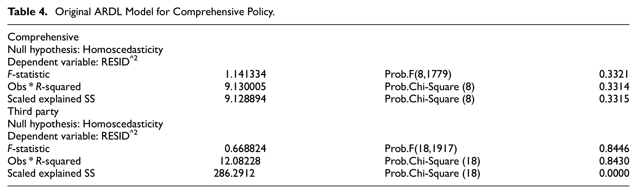
Original ARDL Model for Comprehensive Policy.

Comprehensive
Null hypothesis: Homoscedasticity
Dependent variable: RESID^{^2}
F-statistic	1.141334	Prob.F(8,1779)	0.3321
Obs * R-squared	9.130005	Prob.Chi-Square (8)	0.3314
Scaled explained SS	9.128894	Prob.Chi-Square (8)	0.3315
Third party
Null hypothesis: Homoscedasticity
Dependent variable: RESID^{^2}
F-statistic	0.668824	Prob.F(18,1917)	0.8446
Obs * R-squared	12.08228	Prob.Chi-Square (18)	0.8430
Scaled explained SS	286.2912	Prob.Chi-Square (18)	0.0000

Table 5.

Original ARDL Model for Third Party Policy.

Lag	Comprehensive policies		Third party
	AIC	SIC	AIC	SIC
1	18.14	18.19	12.14	12.18
2	18.15	18.21	12.14	12.19
3	18.14	18.23	12.13	12.21
4	18.15	18.26	12.13	12.22
5	18.15	18.28	12.14	12.24
6	18.15	18.30	12.14	12.26

Before we developed our ARDL model, conditions to satisfy its application in this paper were also very important to be examined. Evidence, for example, has shown that ARDL model would not run if any of the independent variables or the dependent variable is I (2), for detail, see Bahmani-Oskooee and Brooks (2003), Dickey and Fuller (1979, 1981), Engle and Granger (1987), Granger (1983), Granger and Lin (1995), Narayan (2005), Pesaran et al. (2001), Phillips and Perron (1988). Therefore, we performed the Augmented Dickey-Fuller unit root test. As shown in Table 6, all our involving variables in both policy categories under consideration exhibited stationarity at either I (0) or I (1). This is so because, in both the comprehensive and the third-party category, the p-values for all the variables are less than 5% significant level. Moreover, the test statistic in each case is greater than critical values at (1% and 5%) significant levels. Hence, we reject the joint null hypothesis that the variables got unit-roots. Another required condition for the ARDL model application is that there should not be any Heteroskedasticity existence among the involving variables. Thus, all the variables should have equal standard errors (Homoscedasticity). We, therefore, applied the Breusch- Pagan-Godfrey Heteroskedasticity Test, and the results are shown in Table 7. We tested the null hypothesis; there exist Homoscedasticity. In this case, we decide that when the Obs * R-squared value had a p-value of less than .05, then we conclude that there exists Heteroskedasticity, and otherwise, we accept the null hypothesis. As indicated in Table 7, we recorded an Obs * R-squared of 0.3314 and 0.8430 for both Comprehensive and third-party. Comparing these values with the .05 significant level gave us enough evidence to accept our null hypothesis indicating the presence of Homoscedasticity. Also, it is indicated in Figure 1 through the Q-Q plot that our data is normally distributed.

Table 6.

Augmented Dickey-Fuller Unit Root Test for Both Comprehensive and Third-Party Policies.

Dependent variable: D(X1C)	Coeff	Std. error	t-Statistics	p-Value
Sample adjusted: 3 1,791
Included observation: 1,789
Variable
C	1,301.855	324.7915	4.008281	.0001
D(X1C(−1))	0.040940	0.026618	1.538021	.1242
D(X2C(−1))	0.000107	0.000234	0.045928	.9634
D(X3C(−1))	9.408296	9.346439	1.006618	.3143
D(X4C(−1))	−18.80219	18.58411	−1.011735	.3118
D(X5C(−1))	−0.000336	0.001914	−0.175494	.8607
D(X6C(−1))	0.032088	0.045303	0.708310	.4788
D(X7C(−1))	4.853075	3.090008	1.570570	.1165
X1C(−1)	−0.659851	0.050046	−13.18481	.0000
X2C(−1)	−0.001035	0.001398	−0.740278	.4592
X3C(−1)	0.966505	11.70252	0.082589	.9342
X4C(−1)	8.434716	24.78818	0.340272	.7337
X5C(−1)	0.002881	0.002290	1.258310	.2084
X6C(−1)	−0.044064	0.062703	−0.702750	.4823
X7C(−1)	−4.495919	4.380876	−1.026260	.3049
R-squared	0.337935
Adjusted R-squared 0.332710
S.E of regression 2,094.609
F-statistic 64.67833
p-val(F-statistic) 0.000000
Akaike info criterion 18.14047
Schwarz criterion 18.19493

Table 7.

Breusch-Pagan-Godfrey Heteroskedasticity Test.

Dependent variable: D(X1TP)	Coeff	Std. error	t-Statistics	p-Value
Sample adjusted: 1940
Included observation:1936
Variable
C	133.8771	21.78496	6.145394	.000
D(X1TP(−1))	−0.128537	0.041426	−3.102835	.0019
D(X1TP(−2))	−0.092945	0.034700	−2.678557	.0075
D(X1TP(−3))	−0.040077	0.025629	−1.563769	.1180
D(X3TP(−1))	−0.287720	0.550301	−0.522841	.6011
D(X3TP(−2))	0.405868	0.464514	0.873748	.3824
D(X3TP(−3))	0.162014	0.347628	0.466057	.6412
D(X4TP(−1))	−1.918027	0.937775	−2.045295	.0410
D(X4TP(−2))	−1.487033	0.815843	−1.822695	.0685
D(X4TP(−3))	−0.490368	0.621609	−0.788869	.4303
D(X5TP(−1))	0.000127	0.000195	0.0654321	.5130
D(X5TP(−2))	−0.000043	0.000176	−0.024406	.9805
D(X5TP(−3))	−0.000033	0.000147	−0.223981	.8228
D(X6TP(−1))	−0.002557	0.003990	−0.641018	.5216
D(X6TP(−2))	−0.000257	0.003221	−0.079904	.9363
D(X6TP(−3))	−0.001282	0.002295	−0.558733	.5764
D(X7TP(−1))	−0.244327	0.262252	−0.931649	.3516
D(X7TP(−2))	−0.158108	0.214839	−0.735939	.4619
D(X7TP(−3))	−0.132563	0.150684	−0.879742	.3791
D(X1TP(−1))	−0.793782	0.046522	−17.06233	.0000
D(X3TP(−1))	0.473432	0.625758	0.756574	.4494
D(X4TP(−1))	2.584715	1.014546	2.547657	.0109
D(X5TP(−1))	0.000072	0.000187	0.385126	.7002
D(X6TP(−1))	0.001120	0.004669	0.239781	.8105
D(X7TP(−1))	0.404136	0.303532	1.331442	.1832
R-squared	0.457551
Adjusted R-squared 0.450739
S.E of regression 104.2427
F-statistic 67.16313
p-val(F-statistic) 0.000000
Akaike info criterion 12.14415
Schwarz criterion 12.21606

Figure 1.

Normality test for comprehensive in red and third-party in black.

Models Diagnostics Checks

After satisfying all the needed conditions and selected our optimal lags, we then estimate the ARDL for both data groups under consideration and as already mentioned shows the results in Tables 4 and 5 which also depicts the long-run impacts of each independent variable on the dependent variable. We then proceeded to perform some diagnostics check. This was to be sure that the errors in our model are serially not correlated, dynamically stable, and also the existence of long-run relationships. We therefore, in this paper employed serial correlation LM test, Cusum test for stability, and bound test for long-run relationships between our dependent and independent variables. For more details, readers may see, for example, Alhassan and Fiador (2014), Bahmani-Oskooee and Brooks (2003), Emeka and Aham (2016), Narayan (2005), Pesaran et al. (2001), and Phillips and Perron (1988).

First of all, we performed the serial correlation test for both variables category. In Table 8, we show the details of lag one model, which satisfied optimality for the comprehensive policy and lag 3 for a third-party. It is also shown in Table 8 that the probability value of 0.616 for the observed R-squared in the comprehensive case and 0.053 in the third-party case are both above the benchmark value of 5%, indicating that the models satisfy the condition of serial correlation. In Figure 2, we illustrate how our model is stable. As clearly indicated, our models also satisfy the condition of dynamic stability as the blue trend line falls within the boundary of the red lines for both the comprehensive and third-party category. We went ahead to establish long-run relationship amongst our variables. The standard F-statistics from Table 9 are 89.63 and 70.64, respectively, for both comprehensive and third-party categories. These statistics, when compared with Pesaran critical value at 0.05 levels because our models are unrestricted intercept having no trend, indicates significant long-run equilibrium relationship among the involving variables. This is because the standard F-statistics values are far greater than the upper bound value of 3.61 and 3.39, respectively, from the Pesaran Table with p-values of .000 in each case, and hence we reject the null hypotheses in Table 9. See Pesaran et al. (2001) for details.

Table 8.

Breusch-Godfrey Serial Correlation LM test.

Comprehensive lag (1)
Null hypothesis: No serial correlation at up to lag 1	F-statistics	0.248869	Prob.F(1,1773)	0.6179
Sample (N = 1791)	Obs * R-squared	0.251080	Prob.Chi-Square(1)	0.6163
Included observation (1789)
Third party (lag 3)
Null hypothesis: No serial correlation at up to lag 3	F-statistics	12.66409	Prob.F(3,1916)	0.0655
Sample (N = 1940)	Obs * R-squared	37.64243	Prob.Chi-Square(3)	0.0532
Included observation (1938)

Table 9.

Wald Test Result for the Existence of Long Run Relationship Among Variables.

Comprehensive	Null hypothesis: C(9) = C(10) = C(11) = C(12) = C(13) = C(14) = C(15) = 0
		Value	df	p-Value
	F-statistics	89.63014	(7,1,774)	.0000
	Chi-square	627.4110	7	.0000
Third party	Null hypothesis: C(20) = C(21) = C(22) = C(23) = C(24) = C(25) = 0
	F-statistics	70.63685	(5,1911)	.0000
	Chi-square	353.1843	5	.0000

Figure 2.

Stability test for comprehensive (C) and third-party (TP).

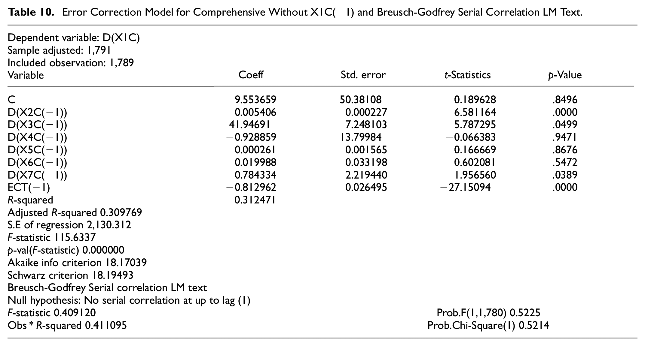
Now, we developed the residual models using our optimal lag (1) and lag (3) for comprehensive and third-parties respectively and illustrate the results in Tables 10 and 11. From Table 10, we show the short-run coefficients using (4) for the regressors a significant value of the residual representing the speed of adjustment of our model at 81.29% toward long-run equilibrium. We then proceed to investigate whether this long-run model satisfies the condition of serial correlation and dynamic stability once again. As it’s shown in Table 10 and Figure 3 respectively, this model has p-value of .521 for theR-squared observed, which implies no serial correlation; however, it’s dynamically unstable. The model dynamic unstable situation, was caused by the lag (1) of our independent variable, and therefore we removed it to ensure that the system is stable as illustrated in Figure 4. The resulting ECT model excluding X1C(−1), as shown in Table 10, also satisfies the condition of serial correlation.

Table 10.

Error Correction Model for Comprehensive Without X1C(−1) and Breusch-Godfrey Serial Correlation LM Text.

Dependent variable: D(X1C)	Coeff	Std. error	t-Statistics	p-Value
Sample adjusted: 1,791
Included observation: 1,789
Variable
C	9.553659	50.38108	0.189628	.8496
D(X2C(−1))	0.005406	0.000227	6.581164	.0000
D(X3C(−1))	41.94691	7.248103	5.787295	.0499
D(X4C(−1))	−0.928859	13.79984	−0.066383	.9471
D(X5C(−1))	0.000261	0.001565	0.166669	.8676
D(X6C(−1))	0.019988	0.033198	0.602081	.5472
D(X7C(−1))	0.784334	2.219440	1.956560	.0389
ECT(−1)	−0.812962	0.026495	−27.15094	.0000
R-squared	0.312471
Adjusted R-squared 0.309769
S.E of regression 2,130.312
F-statistic 115.6337
p-val(F-statistic) 0.000000
Akaike info criterion 18.17039
Schwarz criterion 18.19493
Breusch-Godfrey Serial correlation LM text
Null hypothesis: No serial correlation at up to lag (1)
F-statistic 0.409120		Prob.F(1,1,780) 0.5225
Obs * R-squared 0.411095		Prob.Chi-Square(1) 0.5214

Table 11.

Error Correction Model for Third Party and Breusch-Godfrey Serial Correlation LM Text.

Dependent variable: D(X1TP)	Coeff	Std. error	t-Statistics	p-Value
Sample adjusted: 1940
Included observation: 1936
Variable
C	0.121210	2.386934	0.050780	.9596
D(X1TP(−1))	−0.131103	0.040688	−3.223745	.0013
D(X1TP(−2))	−0.085119	0.034298	−2.481702	.0132
D(X1TP(−3))	−0.036192	0.025393	−1.425243	.1542
D(X3TP(−1))	−0.106351	0.087483	−1.215669	.2243
D(X3TP(−2))	−0.210617	0.100667	−2.092220	.0366
D(X3TP(−3))	−0.267479	0.087123	−3.070124	.0022
D(X4TP(−1))	−6.135090	0.662447	−9.261250	.0000
D(X4TP(−2))	−4.509164	0.681311	−6.618368	.0000
D(X4TP(−3))	−2.028528	0.577538	−3.512372	.0005
D(X5TP(−1))	−0.000090	0.000139	0.648266	.5169
D(X5TP(−2))	−0.000026	0.000150	−0.172388	.8632
D(X5TP(−3))	−0.000047	0.000139	−0.336828	.7363
D(X6TP(−1))	−0.001938	0.001973	−0.982494	.3260
D(X6TP(−2))	0.000188	0.002234	0.084221	.9329
D(X6TP(−3))	−0.001146	0.001972	−0.581085	.5613
D(X7TP(−1))	0.087651	0.131367	0.667221	.5047
D(X7TP(−2))	0.049633	0.152974	0.324457	.7456
D(X7TP(−3))	−0.031019	0.130978	−0.236827	.8128
ECT(−1)	−0.791689	0.045495	−17.40163	.0000
R-squared	0.447942
Adjusted R-squared 0.442467
S.E of regression 105.0247
F-statistic 81.82356
p-val(F-statistic) 0.000000
Akaike info criterion 12.15655
Schwarz criterion 12.21407
Breusch-Godfrey serial correlation LM text
Null hypothesis: No serial correlation at up to lag (3)
F-statistic 12.51464		Prob. F(3,1,913) 0.0655
Obs * R-squared 37.26399		Prob. Chi-Square(3) 0.0532

Figure 3.

Unstable dynamic ECT (C).

Figure 4.

Dynamic stable ECT model (C).

In the third-party case on the other hand, we show in Table 11 the short-run coefficients for the regressors also using (3) a significant value of the residual representing the speed of adjustment of our model at 79.17% toward long-run equilibrium. We then proceed to investigate whether this model in Table 11 satisfies the condition of serial correlation and dynamic stability. From the analysis, the models satisfied both stability and serial correlation test, as illustrated in Figure 5 and Table 11.

Figure 5.

Dynamic stability ECT model (TP).

At this point, after ascertaining the appropriateness of our models, we continue to explore from Tables 10 and 11 for both comprehensive and third-party respectively to establish if there exist short-run effects of our regressors on the dependent variable. Therein, we tested a set of hypotheses in Section 2.3 by employing the Wald test, and the results obtained are illustrated in Table 12 below.

Table 12.

Descriptive Statistics of Explanatory Variables Effects on Premium for Comprehensive (lag 1) and Third Party (lag 3).

Variable	Std. err	Coeff( $β_{i}$ )	F.stats	Chi-square	p-Value
Null hypothesis	Std. err	Coeff( $β_{i}$ )	F.stats	Chi-square	p-Value
Comprehensive (lag 1)
C(2) = 0	0.000821	0.005406	43.31171	43.31171	.0000
C(3) = 0	7.737107	15.18074	3.849718	3.849718	.0499
C(4) = 0	13.99251	−0.928859	0.004407	0.004407	.9471
C(5) = 0	0.001577	0.000548	0.120588	0.120588	.7284
C(6) = 0	0.033368	0.010329	0.095822	0.095822	.7569
C(7) = 0	2.228562	2.131754	5.915008	2.915008	.0089
Third party (lag 3)
C(5) = C(6) = C(7) = 0			7.614425	22.84327	.0000
C(5)	0.323405	−1.462139
C(6)	0.355038	−0.432882
C(7)	0.310594	−0.308952
C(8) = C(9) = C(10) = 0			27.53995	82.61984	.0000
C(8)	0.670729	−6.065143
C(9)	0.688904	−4.267893
C(10)	0.583847	−1.918857
C(11) = C(12) = C(13) = 0			0.321251	0.963754	.8100
C(11)	0.000140	0.000083
C(12)	0.000151	−0.000042
C(13)	0.000140	−0.000093
C(14) = C(15) = C(16) = 0			0.858946	2.576839	.4618
C(14)	0.001981	−0.002524
C(15)	0.002245	−0.000335
C(16)	0.001983	−0.001422
C(17) = C(18) = C(19) = 0			0.268305	0.804915	.8483
C(17)	0.131994	0.101983
C(18)	0.153726	0.084043
C(19)	0.131600	−0.007280

Discussion

Determination of car insurance price impacts policyholder’s decision. Before the insurance premium amount is calculated, the actuary has to consider a lot of rating factors that have bearing effects on the final Premium. These risk-based rating factors are dependent on the specific policyholder. Globally, many attempts have been made, and today’s insurers take into account both technological factors from the insured car and drivers’ characteristics, according to Ayuso et al. (2016). Nevertheless, despite all of these initiatives, the Ghanaian auto insurance market continues to based solely on the age, cubic capacity, use, and inclusion of the sum insured in the comprehensive policy of the vehicle. As a result of the high nature of premiums, policyholders have differing opinions on the factors taken into account (Azaare et al., 2021). To better understand the individual variables impacts on Premium, and call for the introduction of other possible variables for fair premium determination, this paper provides parsimonious explanations on the effect of each classical variable on Premium using data from the Ghanaian insurance market.

After ascertaining the appropriateness of our models, we continue to explore from Tables 10 and 11 for both comprehensive and third parties respectively to establish if there exist short-run effects of our regressors on the dependent variable. In doing so, we tested a set of hypotheses in Section 2.3 by employing the Wald test, and shown in Table 12 is the results obtained. From Table 12, hypothesis C(2) = 0 with F-statistics and significant p-values of 43.3117 and .000 respectively gave us enough evidence to reject our null hypothesis at 5% level. This significant probability value with a positive coefficient is an indication that the sum of the insured car (X2) in the auto insurance market in Ghana has bearing effect in the determination of premiums, meaning Premium is high when the value of the insured car is higher.In effect, policyholders are compensated with the insured autos’ sum once they are able to pay the premium and the insured event happens (Awunyo-Vitor, 2012). In the case of vehicle’s age variable (X3), we illustrated in Table 12 these hypotheses; C(3) = 0 and C(5) = C(6) = C(7) = 0 for comprehensive and third-party respectively. We have F- statistics and p-value of 3.8497, .0499 and 7.6144, .0000 respectively for each category. These significant values at a 5% level also indicate that the vehicle’s age at lag (1) for comprehensive and lag (1)-(3) jointly for the third-party have short-run causality on Premium. Thus, policyholders with older cars pay higher premiums because older cars have high accidents rate (Awunyo-Vitor, 2012; Jacob et al., 2020). This finding which correlates with the markets’ practice contradicts Ayuso et al. (2017), who posits non-linear relationship between auto age and accidents occurences. Moving forward, we consider our next hypotheses for the vehicle’s seating capacity (X4) in both cases as; C(4) = 0 and C(8) = C(9) = C(10) = 0. As indicated in Table 12, the various statistics yielded an insignificant Probability value of 0.9471 supports our null hypothesis acceptance at 5% level. This means that the vehicle’s seating capacity lag (1) has no short-run causality on Premium in the comprehensive case. This finding confirms the reality in the market because cars that are insured with a comprehensive policy are mostly private individuals or corporate, which has no more than five seats and hence does not attract extra charges. However, the third-party category gave us contradictory findings to the former. From Table 12, the F-statistics value of 27.5399 with a significant p-value of .0000 allowed the rejection of the null hypothesis indicating that vehicle’s seating capacity lag (1–3) jointly causes high third-party Premium. The common practice in the market is in a reverse way to the comprehensive insurance, where almost all third-party policies are for commercial purposes with so many seats. This ultimately is the reason for the significant relationship between these two variables in the TP. Generally speaking, vehicles with more seats are bigger, heavier, and less likely to get into accidents (Kahane, 2012; Mela, 1974; Puckett & Kindelberger, 2016). The fact that most comprehensive policies are restricted to a set number of seats, which has no influence on premiums, may be the cause of our inconsistent findings. However, when it comes to third-party policies, our findings are consistent with other research that found a direct link between the severity of claims and premium hikes (Boucher et al., 2009; Jacob & Wu, 2020; Lemaire, 1995; Mert & Saykan, 2005; Sarabia et al., 2004). This finding is most likely explained by the size and mass of third-party vehicles, which frequently are greater in size for commercial purposes and produce severe impact during accidents, leading to high claims and premiums (Kahane, 2012; Mela, 1974; Puckett & Kindelberger, 2016).

Furthermore, when it comes to policyholders claim (X5), several kinds of research have revealed a proportional association between claims and Premium (Ayuso et al., 2017; Bolanc’e et al., 2007; Denuit et al., 2009; Lemaire, 1995; Mert & Saykan, 2005; Sarabia et al., 2004). However, we have a different finding which contradicts our expectation. From the null hypotheses C(5) = 0 and C(11) = C(12) = C(13) = 0 in Table 12, both C and TP were accepted with p-values of .7284 and .8100 at 5% level respectively. This shows an insignificant relationship between premium and claims. We are again not too surprised about this finding concerning the TP, but with the comprehensive, available statistics always proportionate claims increment to premium change (Ayuso et al., 2017). However, we are convinced that this could be as a result of the non-robustness nature of the pricing system used in the market that does not take into consideration severity and frequency of past claims into the premium calculations, see Awunyo-Vitor (2012), Jacob and Wu (2020), and Laryea (2016) for details. Additionally, in the case of vehicle’s cubic capacity (X6), we accepted the null hypotheses: C(6) = 0 and C(14) = C(15) = C(16) = 0 in both category with p-values of .7569 and .4618 respectively at 5% level. This finding supports recent research (Boucher et al., 2013) that found a non-linear connection between vehicle cubic capacity and accident frequency. The most plausible reason for these observations is that the more a car’s horsepower, the greater its acceleration and performance, as well as the longer the distance it travels. Long-distance drivers, without a question, are more at risk. They do, however, become more skilled and experienced as a result of being in their cars for extended lengths of time (Azaare et al., 2021). As a result of their competence and experience, they are less likely to be involved in an accident (Isotupa et al., 2019). Therefore, insurers and policymakers could find other variables more technological in pricing instead of relying on this classical variable, which ends up with high premiums for policyholders just because they have cars with high CC.

Finally, we consider the null hypotheses C(7) = 0 and C(17) = C(18) = C(19) = 0 for policyholder age variable (X7). The F-statistics and the p-value from Table 12 are respectively 5.9150 and .0089. This p-value is significant at a 5% level, and hence we reject the null hypothesis indicating that the age of the policyholder affects comprehensive Premium. Our finding is in line with (Ayuso et al., 2014, 2017; Bolanc’e et al., 2007; McKnight & McKnight, 2003; Nicoletta, 2002). On the contrary, we accepted the null hypothesis in the TP case with a p-value of .8483 at a 5% level, indicating no short-run causality effect from policyholders or drivers age lag (1)–(3) to Premium. From Table 1, policyholders’ mean age in our portfolio is 49 which is an indication of old drivers pricing system.Thus, insurers using this variable could lead to lower premium because older and experience drivers posed lower riks (Ayuso et al., 2014; Azaare et al., 2021). Though there is a contradictory result on this variable effect to Premium for both C and TP, however, according to Ayuso et al. (2014), policies with age elements are mostly targeted on young drivers but yet, there is a report on significant differences between novice and experienced young drivers, indicating heterogeneous risk group among young policyholders. This demonstrates that the risk of claims between older and younger policyholders differ significantly. Premiums are calculated in this scenario based on the policyholder’s age to establish optimal pricing systems (Jacob & Wu, 2020).

Therefore, following these findings, we recommend the inclusion of policyholders age variable into the Ghanaian insurance pricing system whiles autos cubic capacity considering the weight it put on the basic Premium should be re-examined. The policyholder’s driving speed profile, the types of roads they regularly traveled, and the timing are all factors in a conventional insurance pricing scheme.

Conclusion

To better understand the individual variables impacts on Premium, and call for the introduction of other possible variables for fair Premium, we provide in this paper parsimonious explanations on the effect of each classical variable on Premium using data from the Ghanain insurance market in ARDL model. The models developed are dynamically stable, which statistically satisfied the condition of ARDL, and there is well established long-run relationship among dependent and explanatory variables, which are I (0) or I (1). Insurers in the market only based on classical variables such as the auto age, cubic capacity, auto usage, and sum insured in the comprehensive case, which normally results in high premiums for policyholders. The models used in this article has shown that not all the variables that impacts premium used in the pricing system are statistically significant and hence the market need to revise the rating factors (e.g., inclusion of policyholders age, re-examined autos cubic capacity) to obtain an optimal and financially balance pricing model for policyholders.

Managerially, the empirical findings of this paper is to help insurers and government policy makers addressed concerns by policyholders on significant premium determinants for a fair pricing system by understanding the limitations and or opportunities involved in incorporating all other factors involved in auto insurance. According to studies, acquiring new policyholders costs five times more than keeping existing ones (Ampaw et al., 2019; Bhattacherjee, 2001; Chen & Myagmarsuren, 2011). As a result, the findings of this study will serve as a forerunner and policy guide for insurance industry players in developing fair pricing systems by considering only rating factors that have a significant impact on premiums in order to improve policyholders’ retention rates with their various insurers. Also, the article seeks to generate topics for dialog that may provoke interest and discussion on all possible premium determinants within the framework of auto insurance in general. Although the focus of the study is on Ghana, the commonalities in terms of factors considered by insurers in auto insurance premium calculations in the sub-region and globally make our findings transferable.

Due to data limitations, this study was confined to only one insurer and hence, we recommend that future research should be longitudinal and incorporate data from different insurance portfolios. Further, recommending for future studies is understanding omitted variable bias, which this paper tactfully neglected due to analytical approaches used.

Footnotes

Declaration of Conflicting Interests

The author(s) declared no potential conflicts of interest with respect to the research, authorship, and/or publication of this article.

Funding

The author(s) disclosed receipt of the following financial support for the research, authorship, and/or publication of this article: This work was supported by the National Science Foundation of China (project No: 71871044). We also acknowledged Dr. Gabriel Armah of CKTUTAS for proofreading and editing of this paper.

ORCID iDs

Jacob Azaare

Bright Nana Kwame Ahia

References

Aeron-Thomas

(2002). The role of the motor insurance industry in preventing and compensating road casualties: Scoping study (Final report PR/INT/243/02). TRL Limited.

Alhassan

A. L.

(2016). Insurance market development and economic growth: Exploring Causality in 8 selected African countries. International Journal of Social Economics, 43, 321–339.

Alhassan

A. L.

Addisson

G. K.

Asamoah

M. E.

(2015). Market structure, efficiency and profitability of insurance companies in Ghana. International Journal of Emerging Markets, 10, 648–669.

Alhassan

A. L.

Biekpe

(2016). Determinants of life insurance consumption in Africa. Research in International Business and Finance, 37, 17–27.

Alhassan

A. L.

Fiador

(2014). Insurance-growth nexus in Ghana: An autoregressive distributed lag bounds cointegration approach. Review of Development Finance, 4, 83–96.

Amoah

S. K.

Nkrumah-Arkoh

B. P.

(2009). A study of customer satisfaction with service delivery in the motor insurance industry [Master thesis]. Luleå University of Technology.

Ampaw

E. M.

Chai

Frempong

(2019). Examining the overarching factors of clients’ loyalty based on the mobile insurance typology. South African Journal of Business Management, 50(1), a1418. https://doi.org/10.4102/sajbm.v50i1.1418

Awunyo-Vitor

(2012). Comprehensive motor insurance demand in Ghana: Evidence from Kumasi Metropolis. Management, 2(4), 80–86.

Ayuso

Guillen

Jens

P. N.

(2017). Improving automobile insurance ratemaking using telematics: Incorporating mileage and driver behaviour data (Working Paper No. 2017/01). Research Group on Risk in Insurance and Finance. https://link.springer.com/article/10.1007/s11116-018-9890-7

10.

Ayuso

Guillén

Pérez-Marín

A. M.

(2014). Time and distance to first accident and driving patterns of young drivers with pay-as-you-drive insurance. Accident Analysis and Prevention, 73, 125–131.

11.

Ayuso

Guillén

Pérez Marín

A. M.

(2016). Using GPS data to analyse the distance travelled to the first accident at fault in pay-as-you-drive insurance. Transportation Research Part C Emerging Technologies, 68, 160–167.

12.

Azaare

Gumah

Ampaw

E. M.

Kwadwo

S. M.

(2021). Auto insurance premiums in Ghana: An autoregressive distributed lag model approach to risk exposure variables. Journal of Psychology in Africa, 31(4), 362–368.

13.

Azaare

Zhu

Armah

Engmann

G. M.

Kwadwo

S. M.

Ahia

B. N. K.

Ampaw

E. M.

(2022). Measuring the adequacy of loss distribution for the Ghanaian auto insurance risk exposure through maximum likelihood estimation. Open Journal of Business and Management, 10, 846–859. https://doi.org/10.4236/ojbm.2022.102047

14.

Bahmani-Oskooee

Brooks

T. J.

(2003). A new criteria for selecting the optimum lags in Johansen’s cointegration technique. Applied Economics, 35, 875–880.

15.

Bhattacherjee

(2001). Understanding information systems continuance: An expectation-confirmation model. MIS Quarterly, 25(3), 351–370.

16.

Bolanc’e

Michel

Guillen

Lambert

. (2007). Greatest accuracy credibility with dynamic heterogeneity: The Harvey-Fernandes model. Belgian Actuarial Bulletin 7, 14–18.

17.

Boucher

J. P.

Denuit

Guillen

(2009). Number of accidents or number of claims? An approach with zero-inflated poisson models for panel data. The Journal of Risk and Insurance, 76, 821–846.

18.

Boucher

J. P.

Perez-Marin

A. M.

Santolino

(2013). Pay-as-you-drive insurance: The effect of the kilometers on the risk of accident. Anales del Instituto de Actuarios Espaoles, 19, 135–154.

19.

Bülbül

S. E.

Baykal

K. B.

(2016). Optimal bonus-Malus system design in motor third-party liability insurance in Turkey: Negative binomial model. International Journal of Economics and Finance, 8, 205–211.

20.

Chen

C. F.

Myagmarsuren

(2011). Brand equity, relationship quality, relationshipvalue, and customer loyalty: Evidence from the telecommunications. Total Quality Management & Business Excellence, 22(9), 957–974. https://doi.org/10.1080/14783363.2011.593872

21.

Deniut

Mar’echal

Pitrebois

Walhin

J.-F.

(2007). Actuarial modelling of claim: Risk classification, credibility and bonus-Malus scales. Wiley.

22.

Denuit

Xavier

Pitrebois

Walhin

J.-F.

(2009). Actuarial modelling of claim counts risk classification, credibility and bonus-malus systems. John Wiley & Sons.

23.

Dickey

D. A.

Fuller

W. A.

(1979). Distribution of the estimators for autoregressive time series with a unit root. Journal of the American Statistical Association, 74, 427–431.

24.

Dickey

D. A.

Fuller

W. A.

(1981). Likelihood ratio statistics for autoregressive time series with a unit root. Econometrica, 49, 1057–1431.

25.

Duodu

F. K.

Amankwah

(2011). An analysis and assessment of customer satisfaction with service quality in insurance industry in Ghana [Master Thesis in Business Administration, Lulea University of Technology, Department of Business Administration, Technology and Social Sciences].

26.

Edlin

A. S.

(2004). Per-Mile premiums for auto insurance. In Arnott

Greenwald

Kanbur

Nalebuff

(Eds.), Economics for an imperfect world: Essays in honor of Joseph E. stiglitz (pp. 1–68). MIT Press.

27.

Emeka

Aham

K. U.

(2016). Autoregressive Distributed Lag (ARDL)cointegration technique: Application and interpretation. Journal of Statistical and Econometric Methods, 5, 63–91.

28.

Engle

R. F.

Granger

C. W. J.

(1987). Cointegration and error correction: Representation, estimation and testing. Econometrica, 55, 251–276.

29.

Ferreira

Minikel

(2012). Measuring per mile risk for pay-as-you-drive automobile insurance. Transportation Research Record: Journal of the Transportation Research Board, 2297(1), 97–103.

30.

Frangos

N. E.

Vrontos

S. D.

(2001). Design of optimal bonus-malus systems with a frequency and a severity component on an individual basis in automobile insurance. Astin Bulletin, 31(1), 1–22.

31.

Gouri’eroux

Jasiak

. (2004). Heterogeneous INAR(1) model with application to car insurance. Insurance Mathematics and Economics, 34, 177–192.

32.

Ghana National Insurance Commission [NIC]. (2015). Tariff Guide. Insurance Regulator.

33.

Ghana National Insurance Commission [NIC]. (2018). Tariff Guide. Insurance Regulator.

34.

Granger

C. W. J.

(1983). Cointegrated variables and error-correcting models: UCSD (Discussion Paper No. 83-13). Science and Education Academic Publisher.

35.

Granger

C. W. J.

Lin

J. L.

(1995). Causality in the long run. Economic Theory, 11, 530–536.

36.

Isotupa

K. P. S.

Kelly

Kleffner

(2019). Experience-rating mechanisms in auto insurance: Implications for high-risk, low-risk, and novice drivers. North American Journal, 23, 395–411.

37.

Jacob

(2020). An alternative pricing system through Bayesian estimates and method of moments in a bonus-Malus framework for the Ghanaian auto insurance market. Journal of Risk and Financial Management, 13, 143–215.

38.

Jacob

Ahia

B. N. K.

Amankwah

(2020). The over-searching accidents causative factors in Ghana: The role of policyholders education levels. Journal of Economics and Public Finance, 6(1), 8–16.

39.

Kaodui

Mohammed

Yusheng

, et al. (2020). Liquidity and firms’ financial performance nexus: A panel evidence from non-financial firms listed on the Ghana stock exchange (pp. 1–20). SAGE Open.

40.

Kahane

C. J.

(2012). Relationships between fatality risk, mass, and footprint in model year 2000-2007 passenger cars and LTVs. (Final Report, NHTSA Technical Report (DOT-HS[1]811-665)). National Highway Traffic Safety Administration. https://crashstats.nhtsa.dot.gov/Api/Public/ViewPublication/811665

41.

Kelly

Nielson

(2006). Age as a variable in insurance pricing and risk classification. Geneva Papers on Risk and Insurance: Issues and Practice, 31(2), 212–232.

42.

Langford

Koppel

McCarthy

Srinivasan

(2008). In defence of the ‘low-mileage bias’. Accident Analysis and Prevention, 40, 1996–1999.

43.

Laryea

P. N. A.

(2016). Estimating the risk premium of motor insurance in Ghana using the empirical Bayesian credibility theory model [Unpublished Masters thesis]. Kwame Nkrumah University of Science and Technology. http://hdl.handle.net/123456789/9322

44.

Lemaire

(1995). Bonus-malus systems in automobile insurance (Vol. 19, pp. 3–10). Kluwer Academic Publishers.

45.

Lemaire

(1998). Construction of the new Belgian motor third party tariff structure. Wharton School, University of Pennsylvania.

46.

Lemaire

(2004). Bonus-malus systems: In encyclopedia of actuarial science. John Wiley & Sons.

47.

Litman

(2005). Pay-as-you-drive pricing and insurance regulatory objectives. National Association of Insurance Commissioners: Journal of Insurance Regulation, 23, 35–53.

48.

McKnight

A. J.

McKnight

A. S.

(2003). Young novice drivers: careless or clueless? Accident Analysis and Prevention, 35, 921–925.

49.

Mela

D. F.

(1974). “How Safe Can We Be in Small Cars” International Congress on Automotive Safety. (3rd NHTSA Technical Report (DOT HS 801 481)). National Highway Traffic Safety Administration. http://www.nhtsa.dot.go.

50.

Mert

Saykan

(2005). On a bonus-malus system where the claim frequency distribution is geometric and the claim severity is Perato. Hacettepe Journal of Mathematics and Statistics 34, 75–81.

51.

Narayan

P. K.

(2005). The saving and investment nexus for China: Evidence from cointegration tests. Applied Economics, 37, 1979–1990.

52.

Nicoletta

(2002). Driving characteristics of the young and aging population. Statistics Canada.

53.

Osuagwu

E. S.

(2020). Empirical evidence of a long-run relationship between agriculture and manufacturing industry output in Nigeria. Sage Open, 10(1), 1–12.

54.

Paefgen

Staake

Fleisch

(2014). Multivariate exposure modeling of accident risk: Insights from pay-as-you-drive insurance data. Transportation Research Part A Policy and Practice, 61, 27–40.

55.

Paefgen

Staake

Thiesse

(2013). Evaluation and aggregation of pay-as-you-drive insurance rate factors: A classification analysis approach. Decision Support Systems, 56, 192–201.

56.

Pesaran

M. H.

Shin

Smith

R. J.

(2001). Bounds testing approaches to the analysis of level relationships. Journal of Applied Economics, 16, 289–326.

57.

Phillips

P. C. B.

Perron

(1988). Testing for a unit root in time series regression. Bimetrika, 75, 335–346.

58.

Puckett

S. M.

Kindelberger

J. C.

(2016). Relationships between fatality risk, mass, and footprint in model year 2003-2010 passenger cars and LTVs. (Preliminary Report (Docket No. NHTSA- 2016-0068). National Highway Traffic Safety Administration. https://www.nhtsa.gov/sites/nhtsa.gov/files/2016-prelim-%20%20%20%20%20%20%20%20%20%20relationship-fatalityrisk-mass-footprint-2003-10.pdf

59.

Sarabia

J. M.

Gómez-Déniz

Vázquez-Polo

F. J.

(2004). On the use of conditional specification models in claim count distributions: An application to bonus-malus systems. Astin Bulletin, 34, 85–98.

60.

Sivak

Luoma

Flannagan

M. J.

Bingham

C. R.

Eby

D. W.

Shope

J. T.

(2007). Traffic safety in the U.S: Re-examining major opportunities. Journal of Safety Research, 38(3), 337–355.

Exploring the Effects of Classical Auto Insurance Rating Variables on Premium in ARDL: Is the high Policyholders’ Premium in Ghana Justified?

Abstract

Keywords

Introduction

Materials and Methods

Data

The Autoregressive Distributed Lag Model

Testing Long-Run Relationship Presence

Analysis and Results

Ascertaining Data Conformity with ARDL Conditions and Optimal Lag Selection

Models Diagnostics Checks

Discussion

Conclusion

Footnotes

Declaration of Conflicting Interests

Funding

ORCID iDs

References