Sage Journals: Discover world-class research

Abstract

The aim of this study was to comparatively assess the impact of formal and informal finance on household welfare in the Gambia. The Gambia 2015 to 2016 Integrated Household Survey (IHS3) data was analyzed using Stata software version 17.0 to assess the impact of access to the various forms of finance on household food and non-food consumption expenditures, education expenditure, total income, and a subjective assessment of welfare. The study found that access to either formal or informal finance has some deleterious impacts on welfare, with the negative impacts from formal finance being generally lesser than those from informal finance, signaling that the different forms of finance have near-varying repercussions on household welfare. Access to and conditions of formal finance should be improved by removing or making less stringent the requirements, most of which are hard for households to meet.

Keywords

formal and informal finance household welfare PSM The Gambia

Introduction

Background

The Gambia, the smallest country on mainland Africa in terms of land area, has a population of about 2.3 million people ( Gambia Bureau of Statistics [GBoS], 2018). It is highly characterized by a high level of unemployment (35.2%) especially among the youths who are the driving force of an economy. Despite the increasing growth in Gross Domestic Product (GDP) over the years, growing at about 7.2% as of 2018, the poverty rate is high, with up to 48.6% of the population still living under absolute poverty (GBoS, 2017, 2018). This poses a significant threat on the welfare of the population as the high incidence of poverty means lower or irregular incomes, lower spending, lower saving and borrowing, and lower consumption levels, thus leaving the population unable to meet their financial commitments.

According to the 2019 Gambia FinScope survey report, demand for financial services is mainly affected by the ability of the individual to meet the respective financial commitments, and such factors include irregular income levels, low education levels especially on financial products and services, the lack of infrastructure especially in the rural communities and the lack of a financial inclusion strategy in the country (Gambia FinScope, 2019). It is common knowledge that financial inclusion is low in the Gambia, as reportedly only about 31% of 15 years and older members of the population have access to financial services. With up to 69% of the population remaining financially excluded in the country, the picture is much better in other West African countries where only 28% and 36% of the populations of Benin and Nigeria, respectively, are excluded. For the Gambia, evidence has it that individuals who engage in primary activities such as fishing and farming are the most financially excluded, with up to 76% of the population in these activities suffering (Gambia FinScope, 2019). The low level of financial access is also different among geographical areas in the country with a high concentration of banks only based in the urban areas, thereby making most rural households to resort to informal financial services.

Among others, formal financial services in the Gambia include financial access from banks, microfinance institutions (MFIs), village savings and credit institutions (VISACA), cooperative credit unions, and women’s finance association. On the contrary, informal financial access involves lending from traders, and local savings in the societies commonly referred to as “osusu.” Osusu, which is common among women, refers to the process by which members in a particular locality, usually a neighborhood or organization, contribute on stipulated or agreed times mostly monthly or biweekly, a lump sum to one of their members. This person in turn uses the money to meet other spending needs such as buying of household durable or non-durable goods, or the money may be invested, all aimed at improving household welfare.

Many previous studies cite the role of financial access in reducing poverty, eliminating income inequality and ensuring efficient transfer of values thereby promoting consumption smoothening and women empowerment for households. As shown by Quach (2016) and Addury (2018), household access to borrowing and credit is shown to have a significant effect on welfare. This highlights the need for governments of developing countries to take efforts in promoting financial access. Up to date, efforts have been in the pipeline to promote access to financial services in the Gambia, a country which is hit by a low rate of penetration of banks, at about 25% and 5% respectively in urban and rural areas (Jaabi, 2017). Such efforts include the recent drafting of the financial inclusion strategy to guide, regulate, and ensure activities that will enhance and promote financial access to the Gambian populace. In spite of such efforts, there is still more that needs to be understood and done. Interestingly, while up to 62.2% of the population accessed informal credit in 2018, only 38% had access to formal credit. Worse still, use of financial services stands at 12% and 19% for informal and formal services respectively. To effectively direct policy, firstly, there is need to understand the overall impact of access to finance on household welfare for the Gambian economy. More so, there is a need to estimate the differential impact of formal and informal sources of finance as the consequences are expected to be different given the different arrangements involved (see Diagne [1998] for Malawi). Hence the objective of this study is to estimate the welfare effects of access to formal finance and access to informal finance on households in the Gambia. This is achieved by particularly comparing magnitudes of the impacts of access to formal finance and access to informal finance on household welfare in the Gambia, as well as the impact of both forms of finance on households. As such, the findings from this study are not only critical but also timely to policy formulation, especially in terms of the financial inclusion strategy.

This study contributes to the bulk of literature on the role of credit access as a tool for poverty reduction and welfare-enhancement in a liquidity constrained setting. Most recently, making contributions to the debate, a number of studies employed randomized control trials (Banerjee et al., 2015; Breza & Kinnan, 2021; Fink et al., 2020; Meager, 2019) and quasi-experimental techniques (Kaboski & Townsend, 2011; Mwansakilwa et al., 2017), observing that increased access to finance improves consumption, village-level wages, business activity, among other things. In spite of the policy relevance of answers in this debate, no study has been conducted to date to assess the welfare effects of financial access on households in the Gambia. Such a study is important for the development of the financial inclusion strategy which aims at promoting financial development and growth. This study goes beyond the standard practice in the previous quasi-experimental studies by comparing separate impacts of formal finance and informal finance, as well as combined impacts on household welfare using a large cross-section data set. As it stands, most studies in the field only focused on formal finance due to measurement challenges associated with informal finance (such as Amendola et al., 2016). In addition, beyond just using objective welfare measures, this study also employs a subjective measure. Therefore, this paper seeks to fill the existing gap to provide empirical evidence on the differential impacts of financial access, to ensure financial sector development, and hence promote growth and household welfare.

Literature Review

In the literature, several studies have examined the impact of access to finance on household welfare, as measured in various ways. Ideally, the best approach to this task is use of randomized control trials (RCTs) as was done by Breza and Kinnan (2021), Fink et al. (2020), Meager (2019), Banerjee et al. (2015), Angelucci et al. (2015), and Augsburg et al. (2015) among others. Though, due to time and monetary costs, a number of studies still adopt non-experimental methods such as two-stage least squares (2SLS) regression and propensity score matching (PSM) techniques, as was done by Danquah et al. (2020), Addury (2018), Bocher et al. (2017), Mwansakilwa et al. (2017), Amendola et al. (2016), Quach (2016), Kaboski and Townsend (2011), and Diagne (1998), to mention a few. Some of these studies start by identifying the determinants of finance access—such as land holding, household size, savings, and sex of household head—before unearthing the impacts of credit access on the different welfare measures.

One frequently used measure of welfare is household consumption and consumption expenditure, and a number of studies have found credit access to have positive impacts on the measure (Attanasio et al., 2015; Bocher et al., 2017; Fink et al., 2020; Kaboski & Townsend, 2011; Mallick & Zhang, 2019; Meager, 2019; Song et al., 2020). This impact has been observed in various contexts, including in the Mezam district of North-West Cameroon where Atamja and Yoo (2021) found that households that either save formally or informally increase their consumption level, and hence their welfare. Access to finance has also been found to have positive impacts on overall household expenditure in India (Shetty, 2008), household investment in Thailand (Gloede & Rungruxsirivorn, 2013), income (Addury, 2018; Ibrahim & Aliero, 2020; Shetty, 2008), as well as assets and empowerment (Nanziri, 2018; Shetty, 2008).

Access to finance was also found to influence other key outcomes, such as increasing village-level wages (Fink et al., 2020), improving local output prices by inducing delayed selling (Burke et al., 2018), causing modest business creation and expansion (Angelucci et al., 2015; Banerjee et al., 2015; Meager, 2019), and increasing other expenditures (Quach, 2016). Chakrabarty and Mukherjee (2021) used the Theil’s entropy-based index to disaggregate household consumption expenditure into food and non-food items, finding that financial inclusion does not only lead to positive changes in these items, but it also creates a shift from food items to non-food items across households. In the literature, some studies such as Ofori-Abebrese et al. (2020), Hidayat et al. (2021), and Gupta et al. (2014) used the human development index (HDI) as a measure of welfare. Ofori-Abebrese et al. (2020) found that for Sub-Saharan African (SSA) countries, financial inclusion led to an improvement in education of individuals who are included which translates into higher income and thus an improvement in their welfare. Similarly, Hidayat et al. (2021) for Indonesia and Gupta et al. (2014) for India found that financial inclusion does lead to an improvement in the HDI.

Beyond these papers, other studies explored the heterogeneity of impacts—such as Ndlovu and Toerien (2020) who focused on the formal channel and used pooled-household data from 13 sub-Saharan African (SSA) countries, finding that the unconditional effect of access to finance on poverty is non-homogenous, such that the extension of formal finance disproportionately benefits wealthier households more than the very-poor categories.

Conceptual and Theoretical Framework for Access to Finance

In order to better understand how finance access affects economic units, it is worth exploring both the demand and supply sides of the market for credit (Awunyo-Vitor et al., 2014; Beck & de la Torre, 2006). While the demand side of financial services looks at the choices made by economic agents with regards to the services provided by financial institutions, the supply dimension deals with financial intermediation (Awunyo-Vitor, 2018). Among several theories of access to financial services, some relevant ones explain the demand side (including the rational choice theory and the delegated monitoring theory) yet others explain the supply dimension (the information asymmetry theory and the transaction cost theory). With the theory of delegated monitoring contending that intermediaries are delegated to assess information correctly and sufficiently to arrive at sound investment and loan decisions, the approach of the rational choice theory is based on the fundamental principle that choices made by the individual are the best choice to help him/her to achieve set objectives (Awunyo-Vitor, 2018; Diamond, 1984). On the supply side, while the transaction cost theory argues that financial intermediaries emerged to utilize economies of scale as well as transaction technology, the information theory argued that financial services provision is an attempt to overcome costs through improved access to information (Awunyo-Vitor, 2018).

Within the constructs of the demand and supply-side dimensions, it is also worth understanding the context of the credit market especially in less developed economies. First, the credit market has formal and informal segments, whereby the formal segment specializes in savings, credit, and money transfer services or a combination of all, and the informal segment provides only credit services (Awunyo-Vitor, 2018). All these segments work with a rational economic agent, including individuals and households, who always strive to save re-investible funds in order to avoid the cost of credit. They, however, approach the credit market for credit, if they were unable to accumulate enough savings. In addition, Stiglitz and Weiss (1981) describe the lenders’ credit-rationing behavior, which happens to be as a solution to asymmetric information. This happens in the face of high demand and limited supply of credit, resulting from low savings levels and inadequate insurance due to the underdeveloped financial markets (Awunyo-Vitoret al., 2014). As such, some households end up constrained in their access to credit yet others are not constrained in their credit access. Various studies have documented how this setup results in serious credit-constraining of efficient economic agents (see Petrick (2005)).

To better understand the credit market, we adopt a conceptual framework by Awunyo-Vitor (2018) who only focuses on credit access by smallholder farmers. We, therefore, modify it to fit the general household settings. In light of these credit rationing circumstances described above, it can be argued that a household’s decision to apply for financial services and subsequently rationing by the financial intermediary is assumed to be influenced by institutional attributes and the characteristics of the household (Section 1, Figure 1). This results in some households accessing credit, and others failing to get credit (as shown in Section 2 of Figure 1 below), a phenomenon that differentiates resource allocation between the two groups (Section 3, Figure 1) leading to varying productivities (Section 5, Figure 1). Awunyo-Vitor (2018) further conceptualized that agent who use formal financial services are able to relieve liquidity constraints for the purchase of inputs and the cultivation of larger areas (Section 4, Figure 1). Though, how credit access affects productivity and consequently household welfare is worth exploring. With the specification of economic agents as farmers, the concept is summarized in Figure 1 below.

Figure 1.

Conceptual framework of credit access among farming households.

Methodology

Data Description

This study used the Gambia 2015 to 2016 Integrated Household Survey (IHS3) dataset. The 2015 to 2016 IHS is the third round of IHS in the Gambia, following the 2003 to 2004 and the 2010 surveys (GBoS, 2017). This round, compared to the previous two, has a higher response rate (99.4%) and a larger sample as households interviewed were about 13,281. The survey is conducted by the Gambia Bureau of Statistics for a full 1 year with technical assistance from World Bank.

The IHS survey used a two-stage probability proportional to size sampling method. The first stage involved the use of the 2013 Census frame to select Enumeration Areas (EAs), and then a household listing was done on all the selected EAs. The second stage involved using equal probability systematic selection to select 20 households in each of the selected EAs. The survey has four module questionnaires; the first, the household questionnaire that encompassed different sections ranging from household demographic characteristics, labor, education, health, savings and credit, crime, transfers and remittances, and agriculture among others. The second part includes the household consumption expenditure, that is, mainly used for poverty analysis and the third part is the price questionnaire, while the last questionnaire is the community questionnaire for selected communities. The data was analyzed using Stata software version 17.0.

Outcome Variables

In order to get a comprehensive understanding of household welfare, the study adopted as dependent variables both income and consumption patterns following after various previous studies, including Amendola et al. (2016) for Mauritania. This approach is better placed to understand the phenomenon, compared to studies that only include one element of these, such as Quach (2016) for Vietnam. In this case, it is important to adopt both welfare measurements because income shocks may not directly translate into decreased consumption or welfare due to household resilience (Amendola et al., 2016). With inclusion of the role of resilience by measuring consumption, therefore, the study included various welfare indicators (all available in the IHS3 data) including food consumption, non-food consumption, education expenditure, household income, and a subjective assessment of poverty.

Study Design

To compare the impacts of formal and informal financial access on household welfare in the Gambia, the impact evaluation study employed the counterfactual approach of analysis. Three treatment groups (1. households that accessed formal finance only; 2. households that accessed informal finance only; and 3. households that accessed both types of finance) were compared against the control group (households that did not access any finance at all). Drawing from observational data from the Gambia IHS3 survey and given the non-randomization of the data, the study engaged the quasi-experimental study approach, specifically the Propensity Score Matching method (PSM). With the expected large sample from the IHS data the method is expected to yield unbiased and valid estimates. However, the main problem is the fact that access to finance is not random, as households’ access to finance is mainly dependent on their level of income, education, and most times the employment status among others. Thus, to address the possible problem of endogeneity, an instrument was used in this study, as was done by Amendola et al. (2016) and Quach (2016). While the average distance of a household from vital infrastructure and facilities was used as an instrument for formal finance access; informal finance was instrumented by how long (in months) a member of a household lived in the Settlement/Town/Village since his/her last move, or the average income of other households in the community. Thus, in addition to the PSM, the study also used the 2SLS estimation technique, both of which are explained in detail below.

Analytical Approach

Propensity Score Matching (PSM)

To estimate the differential impacts of access to formal and informal finance on household welfare in the Gambia, the study employed impact evaluation (IE) analysis. An impact evaluation basically involves assessing the impact of a program on a set of outcomes of interest. According to Gertler et al. (2016), this involves assessing the causal effect of the program on the outcomes, so as to identify the changes directly attributable to those programs, their modality, or design innovations. This process helps to overcome the challenge of establishing causality by empirically establishing the extent to which a program contributes to the change in outcome (Gertler et al., 2016). The impact of a program (P) on an outcome of interest (Y) can be presented as the difference between the outcome (Y) in the presence of the program and the same outcome (Y) without the program. Mathematically, this can be represented using the IE formula below:

Δ = (Y | P = 1, X) - (Y | P = 0, X)

(1)

For this analysis, the causal impact of finance access (Δ) is the difference between a household’s welfare (Y) after gaining access to either formal or informal finance (i.e., when P = 1) and the same household’s welfare (Y) at the same point in time if the household had not accessed the finance (i.e., when P = 0). This measures a household’s welfare at the same point in time in two different states of the world. Knowing that measuring one household’s different states at the same time is impossible (called the counterfactual problem), IE therefore involves estimating the counterfactual (Y|P = 0), which is treated as the outcome without the treatment.

For a typical program, the causal impact (Δ) of an intervention (P) on an outcome (Y) is the average difference between the outcome (Y) with the program (in other words, when P = 1) and the same outcome (Y) without the program (i.e., when P = 0). The population values of Average Treatment Effect (ATE) and Average Treatment Effect on the Treated (ATET) are therefore defined as;

A T E = E [Δ]

(2)

A T E T = E [Δ | P = 1]

(3)

According to Cameron and Trivedi (2005), while the ATE measure is more relevant when the treatment has universal applicability so that it is reasonable to consider the hypothetical gain from treatment to a randomly selected member of the population, the ATET measure is more relevant when we want to consider the average gain from treatment for the treated. In light of the counterfactual problem, Gertler et al. (2016) point out randomized control trials (RCTs) as the idealistic approach to estimating the counterfactual. However, this is not plausible for this study as use of observational data means that there would be problems of sample selection bias (both on observables and on un-observables). To solve selection on observables, Cameron and Trivedi (2005) propose the matching methods. This study therefore adopted the Propensity Score Matching (PSM) method, which involved obtaining data from a set of potential comparison units that are not necessarily drawn from the same population as the treated units, but for whom the observable characteristics, X, match those of the treated units up to some selected degree of closeness. The mean counterfactual was estimated from the untreated matched group, and the approach solved the evaluation problem by assuming that selection is unrelated to the untreated outcome, conditional on X. The matching ATET estimator (∆M) is given as follows;

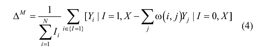
Δ^{M} = \frac{1}{\sum_{i = 1}^{N} I_{i}} \sum_{i \in {I = 1}} [Y_{i} | I = 1, X - \sum_{j} ω (i, j) Y_{j} | I = 0, X]

(4)

where $0 < ω (i, j) < 1$ denote the weight given to the jth case in making a comparison with the ith treated case, and {I = 1} is the set of treated individuals, and j is an element of the set of matched comparison units. The PSM assumes that $ω (i, j) = \frac{1}{N_{C, i}}$ , where $N_{C, i}$ is the number of cases in the comparison group for the ith treated case.

Practically, to estimate the ATET in Stata version 17.0, the study adopted the standard procedure, concisely presented by Harris and Horst (2016). Particularly, the logistic regression was used for calculating propensity scores (p-scores) while picking as many covariates to be used in the model as possible. The following self-selection equations were estimated:

F i n a n c e T y p e_{i} = β + ϑ X + ϵ_{i}

(5)

where $F i n a n c e T y p e_{i}$ is the type of finance under consideration (indicator variables for formal, informal, or both types of finance—each of which was estimated on its own. Particularly, the indicator variable for access to formal finance takes a value one if a household accessed formal finance [from a commercial bank, micro-finance institution, government agency, NGO, and employer, among others] in the 5 years preceding the interview and 0 otherwise; the dummy for informal finance takes a value 1 if a household accessed the finance in the 5 years preceding the interview [from a money lender, trader, farmer, relative/friend/neighbor, and osusu among others], and taking a value of 0 if it did not; while the dummy for both types takes 1 if a household accessed both types, and 0 if not); $X$ is a vector of continuous and dummy covariates (in terms of household head’s sex, age and its square, religion, marital status, education, rural residence; the household’s size, land ownership, disaster affectedness, irrigation farming, and fertilizer use; as well as community disaster affectedness and police availability); and $ϵ$ denotes the error term.

Having created the p-scores, balanced intervention and comparison groups were generated using nearest neighbor (NN) and random draw matching. Balancing is very important in this case because it ensures that each individual has a nonzero probability of participation in the intervention (Austin, 2011). A potential threat to validity to this strongly ignorable treatment assumption is when the balancing property is not attained between the groups for the variables. Given the importance of this assumption, both numerical and visual balance tests were adopted in this study to obtain the highest quality matches (Harris & Horst, 2016; Stuart, 2010). With this commonly used matching technique, computation of the ATT was then restricted to the region of common support.

However, although the PSM helped to deal with the sample selection bias, the approach has several drawbacks, including the fact that it considers only the observable characteristics of units (households) in the matching procedure, thereby ignoring non-observable characteristics. This means that the approach may not deal with the endogeneity problem coming from sample selection bias, where access to finance is not a random process. In this case, the Difference-in-Difference (DID) technique usually comes in handy as it ignores the unobserved individual household characteristics. Though, the technique requires the presence of both baseline and end line data sets, which were not available for these purposes. Therefore, to complement the PSM method, instrumental variables and the two-stage regression method was used. Of course, success of the IV approach heavily depends on the validity of chosen instruments. As such, a thorough search was conducted to identify instruments that are not only valid, but also available in the data set at hand. Consequently, the following econometric regression model was estimated to measure the impacts (each finance type in its own equation):

Y_{i} = α + φ F i n a n c e T y p e_{i} + Θ Z + ε_{i}

(6)

where $Y_{i}$ is the welfare for household i; $F i n a n c e T y p e$ is the dummy variable for the specific form of access to finance; and $Z$ is a vector of characteristics adopted from previous studies; including household-specific variables (such as household size, age of household head, dummy variables for urban or rural location; and household head gender, marital status, and education; Amendola et al., 2016; Quach, 2016). The Greek letters ( $α, φ, Θ$ ) are the parameters that will be estimated and $ε$ denotes a disturbance term which will be considered as heteroskedastic in the analysis.

Instrumental variables technique

Access to finance, both formal and informal, is not a random process, thereby bringing in the problem of endogeneity. According to Amendola et al. (2016), the endogeneity of access to credit could be due to a number of factors, namely: (i) unobserved area-level fixed effects that influence both demand for credit and household income and consumption, such as local prices, infrastructure quality, cultural norms, environmental conditions, and natural-disaster risks; and (ii) unmeasured household characteristics that affect both demand for credit and household income and consumption, such as the health, ability, and fecundity of household members, as well as preference heterogeneity. In the identification of possible instruments, it is worth keeping in mind the existence of credit rationing in the market as a solution to asymmetric information, as well as the high demand and limited supply of credit in rural areas (Akerlof, 1970; Quach, 2016; Stiglitz & Weiss, 1981). Agreeably, this makes the supply of credit to be the one factor that actually matters over all else. Quach (2016) points out in this case that the instrumental variables must, therefore, be those which describe well the characteristics of the lender. While these lender characteristics influence the supply of credit to a household, they do not directly affect the household’s welfare.

Access to formal finance in this study was instrumented based on the concept of the household isolation level (HIL), following after Amendola et al. (2016). For each vital infrastructure and facility (particularly the supply of drinking water, food market, public transportation, primary and secondary school, hospital, health clinic/dispensary, post office, police office, and all seasons road), the survey documented its distance by the most frequent means of transport. For each household, the HIL was then calculated by finding the average distance of the household from the vital infrastructure and facilities. While the HIL is not expected to be correlated with household welfare, it is closely correlated with the amount of formal credit borrowed, or even access to the funds. To ensure robustness of the results, the analysis was repeated by omitting some of the distances to check consistency.

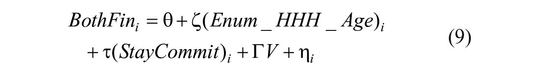
On the contrary, access to informal finance was instrumented by how long (in months) a member of a household lived in the Settlement/Town/Village since his/her last move, because longer stay periods can expand one’s network and increase chances of informal credit while not affecting the household’s welfare. According to Khandker (2003), the amount of credit not only depends on a household’s own characteristics, but also competitors’ characteristics, and hence community-level household characteristics can be used. As such, access to both types of finance was instrumented by the average age of household head in the enumeration area—which is not expected to affect welfare. The household’s intention to stay a year or longer in the community was also used, as it affects the household’s credit commitments but not welfare. Use of competitors’ characteristics as instruments has also been applied by Quach (2017). Using these instruments, the 2SLS econometric technique was used, as follows:

Step 1: Estimate predicted treatment assignments

F o r m a l F i n_{i} = φ + ϑ {(H I L)}_{i} + Ω X + υ_{i}

(7)

I n f o F i n_{i} = ϖ + ω {(S t a y P e r i o d)}_{i} + Λ W + μ_{i}

(8)

\begin{array}{l} B o t h F i n_{i} = θ + ζ (E n u m_H H H_A g e)_{i} \\ + τ (S t a y C o m m i t)_{i} + Γ V + η_{i} \end{array}

(9)

Step 2: Use predicted treatment assignments to evaluate their impacts on household welfare

\begin{array}{l} Y_{i} = α + \propto \hat{F o r m a l F i n_{i}} + Θ Z + ε_{i} \\ Y_{i} = α + φ \hat{I n f o F i n_{i}} + Θ Z + ε_{i} \\ Y_{i} = α + δ \hat{B o t h F i n_{i}} + Θ Z + ε_{i} \end{array}

(10)

where $\hat{F o r m a l F i n_{i}} = \hat{φ} + \hat{ϑ} {(H I L)}_{i} + \hat{Ω} X$ is the predicted access to formal finance; $\hat{B o t h F i n_{i}} = θ + ζ (E n u m_H H H_A g e)_{i} = \hat{I n f o F i n_{i}} = \hat{ϖ} + \hat{ω} {(S t a y P e r i o d)}_{i} + \hat{Λ} W$ is the predicted access to informal finance; $\hat{θ} + \hat{ζ} {(E n u m_H H H_A g e)}_{i} + \hat{τ} {(S t a y C o m m i t)}_{i} + \hat{Γ} Z$ is the predicted access to both types of finance; $Y_{i}$ is the welfare for household i; $υ$ , $μ$ , $η$ , and $ε$ are error terms for Formal finance, Informal finance, Both finance types, and Household welfare regression equations, respectively; HIL represents the calculated household isolation level; StayPeriod is the period in months that a member of a household lived in the Settlement/Town/Village since his/her last move; Enum_HHH_Age is the calculated community average age of household head; StayCommit is a dummy variable for whether the respondent intends to stay for a year or more in the settlement/village/town; the Greek letters ( $φ, ϑ, Ω, ϖ, ω, Λ, θ, ζ, τ, Γ, α, \propto, Θ, δ$ ) are parameters to be estimated; X, W, and V are empirically-backed exogenous variables while Z is a vector for household-specific characteristics. All continuous variables entering the models were logged; and those entering with some zeros were expressed as log $(1 + x)$ , to capture elasticities and to avoid losing observations. The log $(1 + x)$ transformation has been widely applied in the literature by, among others, Carter et al. (2021).

While Equations (7) to (9) define treatment assignment, Equation (10) is for household welfare as a function of the treatments. The two-stage process first involves regressing the three treatment variables on various sets of exogenous variables and instruments. This produces exogenous variation that is not correlated with the error term, so as to address the bias. Predicted values from these equations are then included as regressors in the second stage equation. In order to estimate the predicted values from the first stage, the linear probability model (LPM) was used, rather than the nonlinear discrete models (e.g., probit and logit models). In spite of its weaknesses, the LPM was used because when a nonlinear model is used in the first step, second step estimates are inconsistent unless the first stage model is correct. Predicted values that were greater than or equal to .5 were replaced by 1 and those less than .5 were replaced by 0, implying that these households are potentially beneficiaries and non-beneficiaries, respectively. The instruments were also tested for exogeneity (uncorrelated with the error term in the estimation equation, and correlated with the endogenous regressors) and relevance, using tests of over-identification restrictions, under-identification test, and the weakly identification test (Cameron & Trivedi, 2005). Worth noting is that over-identification tests were only valid for equations estimating the impact of access to both types of finance, because more than one instrument was used in those equations.

Discussion

Household Characteristics, Access to Finance, and Welfare

This section presents the descriptive statistics at household level based on the IHS3 data for the Gambia. Table 1 below summarizes the continuous variables in terms of means and ranges, among others.

Table 1.

Summary Statistics at Household Level.

Variable	Obs	M	SD	Minimum	Maximum
Continuous variables
Expenditures
Food consumption	13,281	85,657	58,792	0	1,445,600
Non-food consumption	13,281	65,436	1,754,109	0	116,000,000
Education	13,281	3,430	7,977	0	277,650
Durable assets	13,281	5,417	20,810	0	1,407,400
Per capita expenditures
Food consumption	13,281	14,235	13,720	0	277,004
Non-food consumption	13,281	13,371	539,134	0	57,800,000
Education	13,281	435	1,188	0	48,265
Durable assets	13,281	762	2,477	0	80,046
Age (years)	13,279	48	14	16	98
Household size	13,281	8	5	1	82
Number of adults	13,281	2	1	1	14
Number of children	13,281	5	4	0	45
Agricultural land (Ha)	13,281	4	23	0	1,400
HH isolation level (HIL, km)	13,281	8	6	0	163
Time taken to amenity (minutes)	13,281	22	14	0	240
Stay period (months)	13,279	491	239	0	1,176
Dummy/categorical variables
Subjective livelihood	13,280	2.19	0.78	1	5
Informal finance access	13,281	0.19	0.39	0	1
Formal finance access	13,281	0.06	0.24	0	1
Finance access	13,281	0.01	0.10	0	1
Sex—Male	13,281	0.85	0.36	0	1
Nationality	13,281	1.16	1.13	1	99
Religion	13,281	0.98	0.13	0	1
Marital status	13,281	2.20	0.95	1	6
Education	13,281	0.48	0.90	0	3
Area of residence	13,281	0.25	0.43	0	1
Disaster-affected community	13,281	0.75	0.43	0	1
Community police/neighborhood	13,281	0.59	0.49	0	1

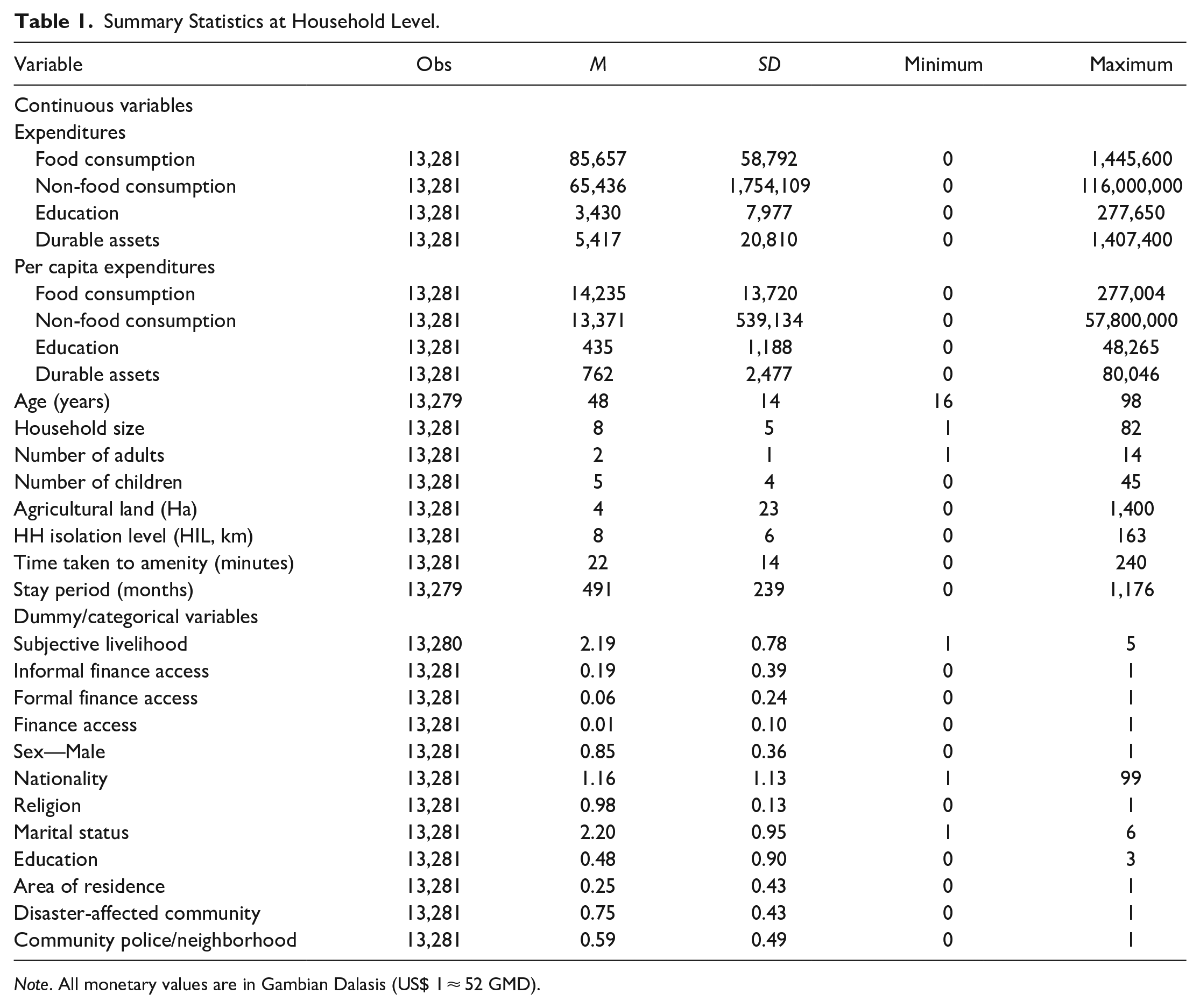
Note. All monetary values are in Gambian Dalasis (US$ 1 ≈ 52 GMD).

The summary statistics show that a typical household head in the Gambia is aged 48 years, has five children, and does agriculture on a 4-Ha piece of land. While the youngest head is aged 16, the oldest head is aged 98 and this head stayed in the village for the entire lifetime. On average, each household spends GMD 85,657 on food and GMD 3,430 on education for all members in a year, and the per capita food and education consumption expenditures are about GMD 14,235 and GMD 435 respectively. A typical home is 8 km away from the nearest social amenity, a distance that is travelled for 22 minutes (one-way). The statistics further show that, demographically, 85% of the heads are male, 98% are Muslims, and 25% live in urban areas. Of these, 75% reported that their community was affected by disasters while 59% reported having the community police or neighborhood. While up to 75% had no education at all (with only 4% receiving some post-secondary training/education), 90% were married, and the sampled population was mostly of Gambian nationality (94%), with other nationalities also living in the country, including the Senegalese (3%), and Guineans (2%) among others. Access to finance was rather low, with only 6%, 19% and 1% obtaining formal, informal, and any finance type respectively. In terms of welfare, Table 2 below decomposes the mean values of consumption and expenditures across credit access.

Table 2.

Mean Income, Consumption, and Expenditure Values Against Finance Access.

Exp./Income	Formal		Informal		Both
Exp./Income	Yes	No	Yes	No	Yes	No
Household level
Food	93,981	85,088	86,070	85,562	110,276	85,391
Non-food	186,225	57,177	35,398	72,388	48,833	65,615
Education	5,610	3,281	2,633	3,615	3,669	3,428
Assets	6,765	5,324	3,699	5,814	5,988	5,410
Per capita values
pc Food	15,262	14,165	12,162	14,715	17,628	14,198
pc Non-food	22,469	12,748	5,132	15,277	8,350	13,425
pc Education	702	417	303	465	522	434
pc Assets	888	753	462	831	1,230	757
Freq. (%)	850 (6.4)	12,431 (93.6)	2,496 (18.8)	10,785 (81.2)	142 (1.1)	13,139 (98.9)

These statistics show that the average food consumption among those who accessed formal finance is GMD 93,981 compared to GMD 86,070 for those who accessed informal finance. Food consumption expenditure, as a measure of welfare is observed to be higher among non-beneficiaries than beneficiaries across all forms of finance. On the contrary, for all the other measures of welfare, beneficiaries of formal finance tend to have higher averages than non-beneficiaries, yet beneficiaries of informal finance have lower welfare than non-beneficiaries. Table 3 below presents further statistics for access across gender against the education levels.

Table 3.

Access to Credit Among Different Sexes at Various Education Levels.

Education	Access to formal finance				Access to informal finance
	Male		Female		Male		Female
	No	Yes	No	Yes	No	Yes	No	Yes
None	8,064	356	1,501	83	6,606	1,814	1,346	238
	95.77	4.23	94.76	5.24	78.46	21.54	84.97	15.03
ECD—primary	628	40	127	11	536	132	119	19
	94.01	5.99	92.03	7.97	80.24	19.76	86.23	13.77
Secondary and non-tertiary	1,438	177	201	17	1,396	219	202	16
	89.04	10.96	92.20	7.80	86.44	13.56	92.66	7.34
Training, tertiary, and postgraduate	421	149	51	17	515	55	65	3
	73.86	26.14	75.00	25.00	90.35	9.65	95.59	4.41
Total	10,551	722	1,880	128	9,053	2,220	1,732	276
	93.60	6.40	93.63	6.37	80.31	19.69	86.25	13.75

Note. Figures are frequencies, with row percentages in decimals.

With 4.23% of male-headed household with no education accessing formal credit, 5.24% of female counterparts accessed the same. Though, the table shows that at higher levels of education the chances of credit are lower for females than males given same education background. The table shows that this gender inequality in access to finance is even worse for informal credit.

In terms of the relationship between finance access and household welfare, Table 4 below shows that access to informal finance declines both for males and females with increasing welfare; that is, less households that rate themselves better in terms of welfare are observed to access informal finance. For example, while 28% of male-headed households that ranked themselves as very poor attained informal finance, only 8% of male-headed rich counterparts accessed finance. The trend is quite different with formal finance, whereby access to finance increases with increasing welfare, though no households that rank themselves as rich actually access formal finance. Statistically, while 6.18% of female-headed very poor households access formal credit, 7.05% of moderately-ranked households accessed the finance. The statistics show that rich households typically prefer to borrow from informal sources to formal ones.

Table 4.

Access to Credit Among Different Sexes at Different Subjective Welfare Levels.

HH welfare	Sex and access to formal finance				Sex and access to informal finance
	Male		Female		Male		Female
	No	Yes	No	Yes	No	Yes	No	Yes
Very poor	2,114	104	349	23	1,592	626	293	79
	95.31	4.69	93.82	6.18	71.78	28.22	78.76	21.24
Poor	4,733	300	785	53	3,961	1,072	699	139
	94.04	5.96	93.68	6.32	78.7	21.3	83.41	16.59
Moderate	3,475	297	672	51	3,276	496	668	55
	92.13	7.87	92.95	7.05	86.85	13.15	92.39	7.61
Fairly rich	216	21	66	1	212	25	64	3
	91.14	8.86	98.51	1.49	89.45	10.55	95.52	4.48
Rich	12	0	8	0	11	1	8	0
	100	0.00	100	0.00	91.67	8.33	100	0.00

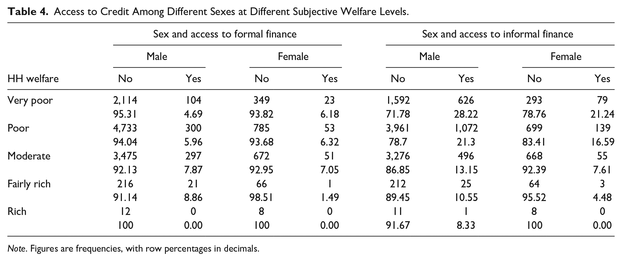
Note. Figures are frequencies, with row percentages in decimals.

Econometric Results

Propensity Score Matching (PSM) Results

Following the methodology and data exploration above, this section presents the econometric findings, starting with those from the PSM approach. As a key step after generating p-scores using the logistic regression in Stata, numerical, and visual balance tests were conducted to assess the quality of matches obtained, so as to check whether the propensity score adequately balances characteristics between the treatment and comparison group units. For formal finance, informal finance, and both finance types, Tables 5 to 7, respectively, present the balance tests between the groups.

Table 5.

Balance Tests Between Treatment and Comparison Groups for Formal Finance.

	Means before matching			Means after matching
	Without	With	Diff	Without	With	Diff
Sex	1.151	1.151	0.001	1.121	1.141	–0.020
Age (years)	3.825	3.824	0.001	3.871	3.864	0.007
Age—Sq	14.726	14.700	0.026	15.061	14.999	0.062
Household size	1.861	1.906	–0.045*	2.136	2.143	–0.007
Religion—Christianity	1.016	1.024	–0.007	1.012	1.012	0.000
Married	0.899	0.906	–0.007	0.921	0.925	–0.003
Divorced	0.011	0.014	–0.003	0.005	0.003	0.002
Separated	0.002	0.005	–0.003	0.005	0.003	0.002
Widowed	0.053	0.049	0.003	0.052	0.057	–0.005
Edu–ECD and primary	0.061	0.060	0.001	0.052	0.062	–0.010
Edu—secondary and non-tertiary	0.132	0.228	–0.096***	0.181	0.169	0.012
Edu— >training, tertiary	0.038	0.195	–0.157***	0.117	0.121	–0.003
Area—rural	1.753	1.684	0.070***	1.838	1.849	–0.012
Land size (Ha)	4.105	3.653	0.452	5.056	5.179	–0.123
Disaster affected	0.111	0.151	–0.039***	0.204	0.198	0.007
Community disaster	0.748	0.754	–0.007	0.888	0.864	0.023
Community police	0.582	0.656	–0.075***	0.564	0.588	–0.023
Irrigation farming	0.101	0.143	–0.043***	0.157	0.139	0.018

p < .10. **p < .05. ***p < .01.

Table 6.

Balance Tests Between Treatment and Comparison Groups for Informal Finance.

	Means before matching			Means after matching
	Without	With	Diff	Without	With	Diff
Sex	1.161	1.111	0.050***	1.139	1.079	0.060**
Age (years)	3.824	3.832	–0.008	3.872	3.839	0.033
Age—Sq	14.714	14.766	–0.052	15.065	14.807	0.258
Household size	1.828	2.017	–0.189***	2.125	2.232	–0.107**
Religion—Christianity	1.019	1.007	0.012***	1.012	1.012	–0.001
Married	0.891	0.934	–0.043***	0.919	0.945	–0.026
Divorced	0.012	0.006	0.006**	0.005	0.000	0.005
Separated	0.003	0.002	0.001	0.005	0.000	0.005
Widowed	0.055	0.039	0.017***	0.058	0.030	0.028
Edu—ECD and primary	0.061	0.060	0.000	0.061	0.030	0.031
Edu—secondary and non-tertiary	0.148	0.094	0.054***	0.180	0.146	0.033
Edu— >training, tertiary	0.054	0.023	0.031***	0.120	0.110	0.011
Area—rural	1.718	1.883	–0.165***	1.832	1.915	–0.083***
Land size (Ha)	3.816	5.200	–1.384***	5.068	5.427	–0.359
Disaster affected	0.101	0.170	–0.070***	0.187	0.287	–0.099***
Irrigation farming	0.110	0.080	0.030***	0.150	0.140	0.009

p < .10. **p < .05. ***p < .01.

Table 7.

Balance Tests Between Treatment and Comparison Groups for Both Types.

	Means before matching			Means after matching
	Without	With	Diff	Without	With	Diff
Sex	1.151	1.127	0.025	1.129	1.182	–0.053
Age (years)	3.825	3.810	0.015	3.868	3.853	0.015
Age—Sq	14.726	14.590	0.136	15.032	14.944	0.088
Household size	1.863	1.924	–0.061	2.140	2.138	0.001
Religion—Christianity	1.017	1.021	–0.004	1.012	1.000	0.012
Married	0.899	0.915	–0.016	0.924	0.879	0.045
Divorced	0.011	0.028	–0.017*	0.003	0.030	–0.027**
Separated	0.002	0.007	–0.005	0.004	0.000	0.004
Widowed	0.053	0.028	0.024	0.054	0.061	–0.006
Edu—ECD and primary	0.061	0.056	0.004	0.057	0.061	–0.004
Edu—secondary and non-tertiary	0.138	0.155	–0.017	0.174	0.212	–0.038
Edu— >training, tertiary	0.048	0.014	0.034*	0.121	0.030	0.091
Area—rural	1.749	1.782	–0.033	1.842	1.879	–0.036
Land size (Ha)	4.075	4.133	–0.057	5.147	4.086	1.060
Disaster affected	0.114	0.120	–0.006	0.205	0.061	0.144**
Community disaster	0.747	0.859	–0.112***	0.879	0.788	0.091
Community police	0.586	0.613	–0.026	0.574	0.667	–0.093
Irrigation farming	0.103	0.129	–0.026	0.147	0.182	–0.035
Fertilizer use	0.593	0.663	–0.070	0.665	0.727	–0.062

p < .10. **p < .05. ***p < .01.

These balance test results broadly show that the respective comparison groups have distributions of propensity scores similar to the respective intervention groups; that is, mean differences are generally no longer statistically significant after matching. Particularly, Table 5 shows that although statistical differences exist in the whole sample (before matching) for education, rural residence, disaster affectedness, irrigation farming, and presence of community police, the matched pairs show no statistical differences for these and the rest of the variables. Significant improvements are also observed for informal finance and both types of finance after matching. Overall, the test of balancing property of the propensity score is satisfied for all three types of finance. These findings are cemented by a visual diagnosis of balance as conducted using Kernel densities, depicted by Figure 2 below which captures each finance type per row.

Figure 2.

Distributions of propensity scores for different types of finance.

For all three rows in the figure above (respectively, capturing each finance type), it is evident that densities of the propensity scores are more similar after the matching as the second column has only limited (or no) overlap between the groups. By passing the balancing test, the matches can be used with confidence to estimate the impact of finance on welfare. PSM estimation results are presented in Table 8 below.

Table 8.

Propensity Score Matching Estimation Results.

Finance	Food		Non-food		Education		Income		Subjective
Finance	ATT	t-stat	ATT	t-stat	ATT	t-stat	ATT	t-stat	ATT	t-stat
Formal	0.062	1.674*	0.153	2.772***	0.350	1.581	0.352	4.463***	–0.029	–0.619
Informal	0.017	0.841	0.141	4.392***	–0.062	–0.475	0.071	1.530	–0.214	–8.424***
Both	0.222	2.602**	0.316	2.533**	0.930	1.705*	0.771	4.218***	0.109	0.938

Note. ATT is the Average Treatment Effect on the Treated, also abbreviated ATET.

p < .10. **p < .05. ***p < .01.

With the principal objective being to examine the impact of access to finance on household welfare, three treatment groups were employed: access to formal finance; access to informal finance; and access to both types of finance. Holding everything constant, Table 8 above shows that households were better off after accessing formal finance than before, in terms of expenditures on non-food items and improvements in income, yet formal finance has no impact on food consumption and education expenditures as well as subjective poverty at the 5% level of significance. Particularly, the ATT shows that if households that accessed formal finance did not access the finance they would have had 15% less non-food consumption and 35% less total incomes. Essentially, this means that access to formal finance improves household non-food consumption expenditure and income. This finding makes sense considering the restrictions that formal credit sources place on use of funds, in favor of investments rather than consumption. In fact, in order to ensure loan repayment, formal credit sources in the Gambia typically favor credit for income-generating activities over food consumption for most loans (Zeller et al., 1994).

In the same vein, the results in Table 8 show that access to informal finance improves welfare in terms of non-food consumption spending (14%), yet the ATT shows that if households that accessed informal finance did not access the finance they would have had a 21% higher rating for their subjective assessment. This means that informal finance has a negative effect on subjective livelihood. Given that this welfare measure is based on a household’s own comparison with other community members, it makes sense that access to informal loans makes households rate themselves lower. The effect of household access on both types of finance is significant and positive for food and non-food expenditures, total income, and subjective livelihood assessment. This huge magnitude serves to encourage financial inclusion as a way of improving household welfare as found by Mallick and Zhang (2019). Particularly, PSM results show that households are less likely to be poor if they have access to financial services, implying that if households are encouraged to access finance, they will improve on their spending patterns as well as have more avenues to create more wealth through an increase in income. However, the PSM may be faulted for increasing imbalance, inefficiency, model dependence, and bias (King & Nielsen, 2019). As such, the instrumental variables technique was also used, and its results are presented in the section below.

Instrumental Variables (IV) Regression Results

As described above, this approach involved a two-step procedure, as follows: (i) estimating predicted treatment assignments; and (ii) using predicted treatment assignments to evaluate their impacts on household welfare. Dependent variables in the first step were access to formal finance, access to informal finance, and access to both types of finance. These were regressed on the proposed instrumental variables (household isolation level for formal finance; number of months the household has stayed in community since last move for informal finance; and average age of household head in community as well as intention to stay for both types of finance) in the presence of some control variables as suggested by credit theory and practice, while attaining the right model specification. Table 9 below presents the results from this stage.

Table 9.

LPM Estimation of Access to Finance.

Variable	Formal finance	Informal finance	Both forms
Female	–0.009 (0.009)	–0.022* (0.013)	–0.007 (0.004)
Log (age, years)	0.543*** (0.133)	0.778*** (0.236)	0.092 (0.063)
Log (age) squared	–0.073*** (0.017)	–0.110*** (0.031)	–0.013 (0.008)
Christianity	0.014 (0.021)	–0.029 (0.023)	0.003 (0.009)
Log (number of adults)	–0.010 (0.008)	0.004 (0.013)	–0.004 (0.004)
Log (number of children)	0.013*** (0.004)	0.020*** (0.006)	0.002 (0.002)
Log (land size, Ha)	0.001 (0.003)	0.040*** (0.005)	0.000 (0.002)
Rural residence	–0.019*** (0.007)	0.067*** (0.010)	–0.001 (0.003)
Marital status
Married	0.008 (0.013)	–0.002 (0.019)	0.002 (0.006)
Divorced	–0.002 (0.025)	0.008 (0.034)	0.012 (0.014)
Separated	0.097 (0.074)	0.031 (0.080)	0.032 (0.041)
Widowed	0.004 (0.017)	–0.000 (0.025)	–0.003 (0.008)
Irrigation farming	0.027*** (0.009)	–0.042*** (0.013)	0.001 (0.004)
Log (HIL)	–0.010** (0.004)
Fertilizer use		–0.002 (0.008)	–0.001 (0.002)
Education
ECD—primary		0.004 (0.015)	–0.006* (0.004)
Secondary—non-tertiary		–0.031*** (0.010)	–0.001 (0.004)
Training-tertiary-postgraduate		–0.049*** (0.014)	–0.009** (0.004)
Average HH income in comm.		–0.004 (0.006)
Log (stay period [months])		0.014*** (0.004)
Log (HHH age in Enum)			0.035*** (0.009)
Intend to stay in comm			–0.007* (0.004)
_cons	–0.906*** (0.251)	–1.361*** (0.451)	–0.263** (0.120)
F	5.758	30.454	2.067
p-Value	.000	.000	.004
N	12,413	12,404	10,531

Note. Heteroskedasticity-robust standard errors in parentheses.

p < .10. **p < .05. ***p < .01.

In terms of the determinants of access to formal finance, the results show that age of the head of the household positively determines access to finance, at a decreasing rate. The number of children a household has and irrigation farming significantly influence a household’s access to formal credit positively. Though, rural residence and the average distance from key amenities negatively influence access to formal finance. These observations were also made by Amendola et al (2016) for Mauritania. Among the significant determinants of access to informal finance is the number of months a household stays in the community since its last move, and household’s area of residence, land size, irrigation farming, education level, and number of children, whereby rural households and those with more children and land are more likely to access informal finance, yet households that do irrigation farming and have more educated heads are less likely to access informal credit compared to their counterparts. This is in line with findings by Quach (2017). For access to both forms of finance, the results indicate as significant determinants education of the household head, as well as the average age of household head in the enumeration area. More broadly, the results show that there is a divide in credit access in the sample, whereby rural households rely mostly on informal credit, likely due to low supply of formal finance; yet, more commercial households that are involved in irrigation farming make recourse to formal finance. The rural-urban dichotomy was also recently observed by World Food Programme & Vulnerability Analysis and Mapping (2016).

With these first stage regression results, second stage results were then estimated. At this stage, three key diagnostic tests were conducted: test of endogeneity, test of weak identification, and instruments’ explanatory power, and the test of overidentifying restrictions (respectively’ using “estat endogenous,” “estat firststage, all,” and “estat overid” in Stata 17.0). In all models of formal and informal finance access, the robust score chi-square and robust regression F-statistics were all significant at 5% level of significance, indicating that the null of exogeneity is rejected, so that the finance access variables are indeed endogenous. In terms of the weak identification test which is aimed at checking whether the instruments are jointly significant (and to test instruments’ explanatory power), the rule of thumb states that a model is weakly identified if the first stage F-statistic is below a rule of thumb of 10 (Staiger & Stock, 1997; Stock & Yogo, 2005). In this case, weak instruments may cause instrumental-variables estimators to be biased, and hypothesis tests of parameters estimated by instrumental-variables estimators may suffer from severe size distortions (Stock & Yogo, 2005). For all the estimated models, statistically significant F-statistics were achieved, and hence it was concluded that the used instruments are not weak. Another important test that was conducted for models with more than one instrument is the test of overidentifying restrictions, which tests whether the instruments are uncorrelated with the error term, and whether the equation is mis-specified such that one or more of the excluded exogenous variables should in fact be included in the structural equation. A significant test statistic in this regard represents either an invalid instrument or an incorrectly specified structural equation. The estimated models in this study had statistically insignificant statistics, with the structural models specified to have various control variables.

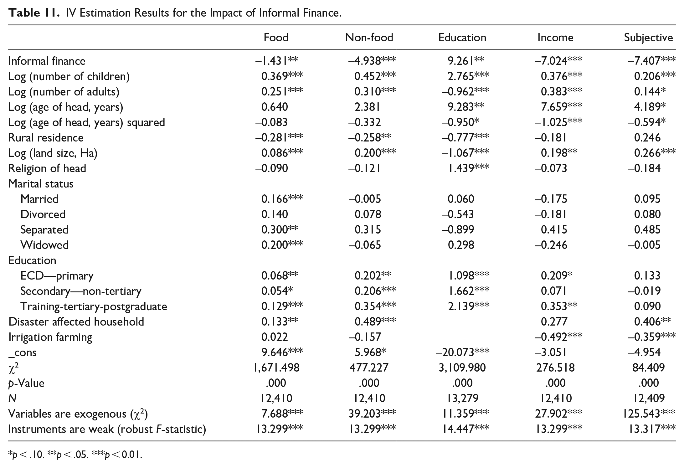
After checking all necessary diagnostic tests, the five welfare measures (food consumption expenditure, non-food consumption expenditure, education expenditure, total household income, and the subjective livelihood assessment measure) were then modeled using the IV approach to see the impact of access to the different types of finance (instrumented by household isolation level, stay period in the community as well as average age of household heads in the enumeration area, and intention to stay longer). Tables 10 to 12 below present the IV estimation results for formal finance, informal finance, and both types of finance, respectively, and their respective diagnostic test results.

Table 10.

IV Estimation Results for the Impact of Formal Finance.

	Food	Non-food	Education	Income	Subjective
Formal finance	4.670**	17.043***	63.105***	5.475*	–4.766**
Log (number of children)	0.268***	0.116	1.883***	0.168***	0.113***
Log (number of adults)	0.338***	0.409***	0.412	0.252***	0.081
Sex of head	0.133***	0.102	1.387**	–0.126*	0.064
Religion of head	–0.122	–0.188	0.069	0.164	0.200
Log (age of head, years)	–2.781**	–11.518***	–20.002	–1.671	1.031
Log (age of head, years) squared	0.378**	1.523***	2.847	0.229	–0.150
Rural residence	–0.214***	–0.049	1.743*	–0.453***	–0.436***
Log (land size, Ha)	0.033**	0.015	–0.706***	–0.084***	–0.048**
Irrigation farming	–0.036	–0.367*	–0.746	–0.315***	0.097
Disaster affected household	–0.085	–0.327	–1.281*	–0.369***	–0.025
Disaster affected community	–0.121***	–0.295**	–1.163**	–0.241***	0.056
_cons	15.674***	30.552***	29.338	13.792***	0.996
χ²	684.001	91.345	226.915	473.685	139.564
p-Value	.000	.000	.000	.000	.000
N	12,410	12,410	12,410	12,410	12,409
Variables are exogenous (χ²)	23.619***	140.410***	135.819***	4.775**	18.628***
Instruments are weak (robust F-statistic)	7.358***	7.358***	7.358***	7.358***	7.363***

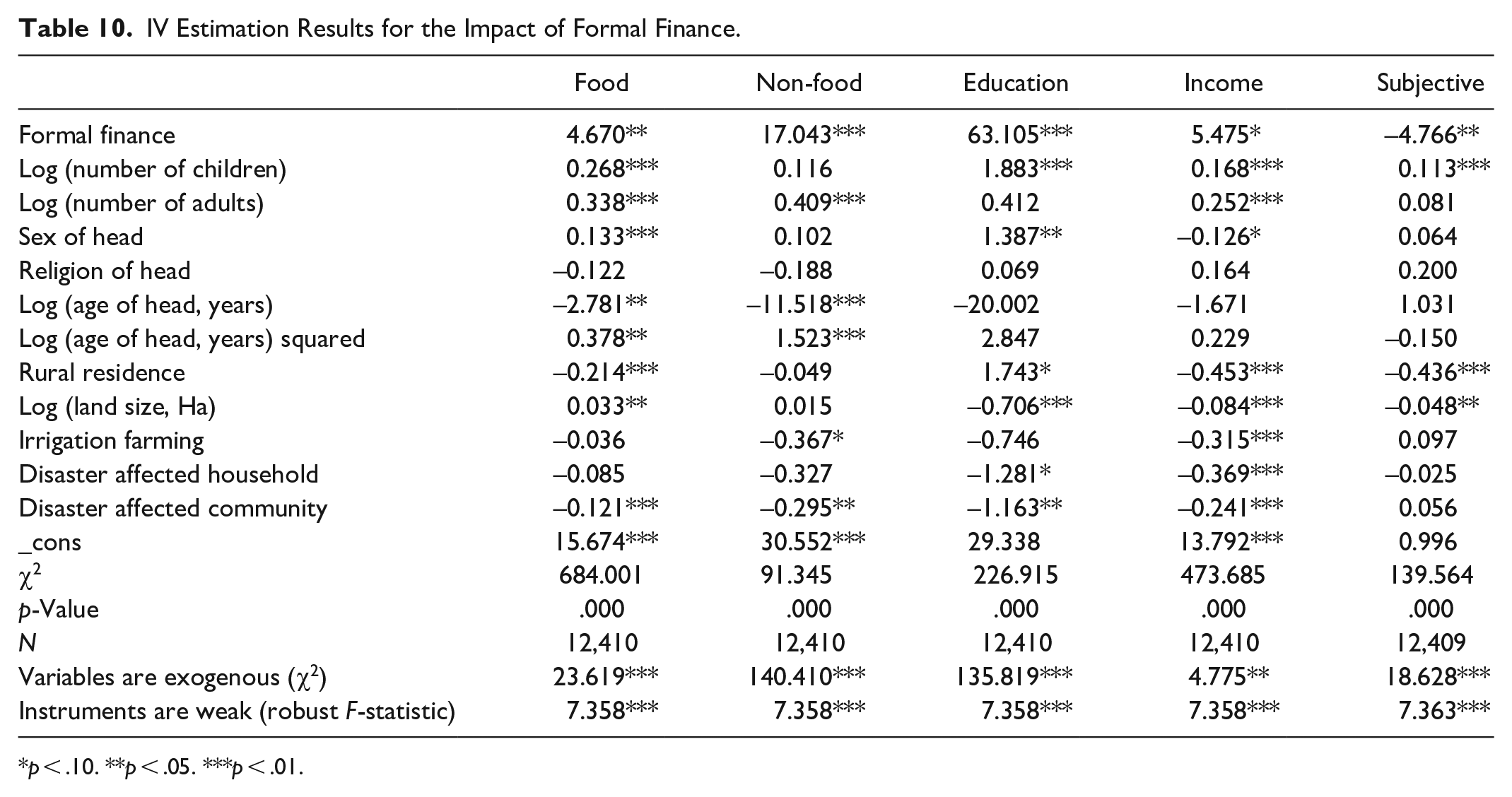
p < .10. **p < .05. ***p < .01.

Table 11.

IV Estimation Results for the Impact of Informal Finance.

	Food	Non-food	Education	Income	Subjective
Informal finance	–1.431**	–4.938***	9.261**	–7.024***	–7.407***
Log (number of children)	0.369***	0.452***	2.765***	0.376***	0.206***
Log (number of adults)	0.251***	0.310***	–0.962***	0.383***	0.144*
Log (age of head, years)	0.640	2.381	9.283**	7.659***	4.189*
Log (age of head, years) squared	–0.083	–0.332	–0.950*	–1.025***	–0.594*
Rural residence	–0.281***	–0.258**	–0.777***	–0.181	0.246
Log (land size, Ha)	0.086***	0.200***	–1.067***	0.198**	0.266***
Religion of head	–0.090	–0.121	1.439***	–0.073	–0.184
Marital status
Married	0.166***	–0.005	0.060	–0.175	0.095
Divorced	0.140	0.078	–0.543	–0.181	0.080
Separated	0.300**	0.315	–0.899	0.415	0.485
Widowed	0.200***	–0.065	0.298	–0.246	–0.005
Education
ECD—primary	0.068**	0.202**	1.098***	0.209*	0.133
Secondary—non-tertiary	0.054*	0.206***	1.662***	0.071	–0.019
Training-tertiary-postgraduate	0.129***	0.354***	2.139***	0.353**	0.090
Disaster affected household	0.133**	0.489***		0.277	0.406**
Irrigation farming	0.022	–0.157		–0.492***	–0.359***
_cons	9.646***	5.968*	–20.073***	–3.051	–4.954
χ²	1,671.498	477.227	3,109.980	276.518	84.409
p-Value	.000	.000	.000	.000	.000
N	12,410	12,410	13,279	12,410	12,409
Variables are exogenous (χ²)	7.688***	39.203***	11.359***	27.902***	125.543***
Instruments are weak (robust F-statistic)	13.299***	13.299***	14.447***	13.299***	13.317***

p < .10. **p < .05. ***p < 0.01.

For all the three tables above, the null hypotheses that variables are exogenous and that used instruments are weak are rejected at the 5% level. This implies that the treatment variables are indeed endogenous and hence the IV estimator is better than the OLS estimator, and the used instruments are good. For Table 12, the null hypothesis that overidentifying restrictions are valid is not rejected and hence the used instruments are valid and the models are correctly specified. The regression results in Table 10 above show that access to formal finance is welfare-depressing for the subjective measure, and welfare-enhancing for the remaining four measures. This is in line with the PSM results presented above, especially for non-food expenditure and total income. Also, the results corroborate those by Quach (2016), Addury (2018), and Song et al. (2020) who found a significant and positive effect of household access to formal finance on welfare, as well as Danquah et al. (2020) who found that households are less likely to be poor if they have access to financial services.

Table 12.

IV Estimation Results for the Impact of Both Types of Finance.

	Food	Non-food	Education	Income	Subjective
Both finance types	–6.745***	8.339**	69.582***	–23.396***	–12.560***
Log (number of children)	0.354***	0.336***	2.843***	0.267***	0.091***
Log (number of adults)	0.218***	0.262***	–0.729***	0.250***	0.022
Log (age of head, years)	0.258	–2.009**	8.050	4.574**	–0.263
Log (age of head, years) squared	–0.030	0.277**	–0.810	–0.595**	0.025
Rural residence	–0.400***	–0.659***	–0.453*	–0.652***	–0.250***
Christianity	–0.012	0.036	0.964	0.204	0.046
Marital status
Married	0.199***	–0.001	–0.057	–0.182	0.132
Divorced	0.311**	–0.001	–0.846	–0.017	0.177
Separated	0.506	0.084	–2.135	0.866	0.624
Widowed	0.181**	0.023	0.654	–0.438**	–0.018
Education
ECD—primary	0.022	0.251***	1.447***	0.057	0.060
Secondary—non-tertiary	0.090***	0.353***	1.287***	0.288***	0.222***
Training-tertiary-postgraduate	0.145***	0.701***	2.162***	0.532***	0.400***
Log (land size, Ha)	0.014	–0.023	–0.879***	–0.092*	–0.050*
Fertilizer use	0.120***	0.273***	0.817***	0.059	0.112***
Irrigation farming	0.086***	0.019	0.577**	–0.193*	–0.025
_cons	10.378***	13.780***	–17.727*	2.720	3.072
χ²	1,103.398	1,252.640	1,154.988	278.059	280.417
p-Value	.000	.000	.000	.000	.000
N	10,531	10,531	10,531	10,531	10,530
Variables are exogenous (χ²)	19.273***	6.222**	50.500***	38.075***	30.995***
Instruments are weak (robust F-statistic)	7.710***	7.710***	7.710***	7.710***	7.709***
Overidentifying restrictions are valid (χ²)	0.670	2.253	1.364	0.011	2.021

p < .10. **p < .05. ***p < .01.

Interestingly, access to informal finance has a negative impact on up to four household welfare measures (with the exception of education expenditure). This is especially worse when welfare is defined subjectively or by household income, in which case informal finance reduces household welfare by up to 700%, other things held constant. This welfare-depressing impact on households could be explained by the stringent collateral rules, and the non-accommodative trends in informal finance, which sometimes see households’ properties being confiscated due to delayed payments or default. Also cause for concern with the results could be the usurious interest rates in the Gambia, which reach as high as 30% on the formal market and more than 100% on the informal market (Zeller et al., 1994). These high interest rates are especially bad for households which mainly borrow for consumption. In fact, the negative coefficients found in this study could explain the low savings and investment propensities, whereby only 4% of the population save or invest as reportedly 51% and 42% of the population claim that they do not have income to spare or do not have any remaining money after spending for livelihood, respectively (Gambia FinScope, 2019).

In terms of access to both forms of finance, the IV estimation results find positive impacts on non-food and education expenditures, and negative impacts on food expenditure, total income, and the subjective measure. While the result for non-food expenditure is in line with PSM results in Table 8 above, the findings are different for the other measures pointing out to the probable bias that comes in with PSM, as pointed out by King and Nielsen (2019). More broadly, the results show that access to informal finance is more welfare-harming than access to formal finance, probably because interest rates are generally higher and conditions more unfavorable in informal than formal settings. Given the prominence of informal finance amidst a thin formal credit market, there is need to incentivize supply of formal loans across all areas.

Conclusion

This study examined the differential impacts of access to formal and informal finance for the Gambia using the IHS3 survey data. PSM and IV estimation techniques were employed on the 13,281 sampled households. Interestingly, access to both formal and informal finance was found to have some deleterious impacts on welfare, contrary to what was observed in other countries (such as Bocher et al., 2017 for Ethiopia and Quach, 2017 for Vietnam). Particularly, the study found that in spite of its ease of access and wide availability, informal finance is in fact far from being a panacea for welfare enhancement, causing harm on almost all welfare measures. This negative impact is much worse on household income where it leads to a 740% loss of income. The negative impacts from formal finance are generally lower than those by informal finance, signaling that the different forms of finance have near-varying repercussions on household welfare, with formal finance being the lesser evil. Various policy issues arise from the findings, both from the supply side and from the demand side. Most importantly, given that formal finance is less welfare-depressing (and of course welfare-enhancing in the PSM results), there is need to improve access to and conditions of formal finance by removing or making less stringent the requirements, most of which are hard for households to meet. Once this is done, households should be encouraged to access formal finance, which will result in improvements in their spending patterns, so as to have more avenues to create more wealth through an increase in income. To support the demand side, there is need to enhance the flow of information to the citizenry on the available formal finance services to improve uptake of the same. Possible regulation of the environment in which informal credit access occurs is also important, in order to ensure that households, which usually have little information, are not taken advantage of. Limitations with the use of quasi-experimental tools in this study call for further analyses using field experiments which can aid with precision on how, and under what conditions financial services benefit poor people. In fact, given the existing divide in access to finance across people of different demographic characteristics, impacts of the different forms of finance could differ between males and females, for example. Future research could unearth such heterogeneities. An interesting direction for further research could also be to establish whether the two forms of finance are actually substitutes or complements.

Footnotes

Availability of Data and Materials

The data used in this study is publicly available on the domain

Declaration of Conflicting Interests

The author(s) declared no potential conflicts of interest with respect to the research, authorship, and/or publication of this article.

Funding

The author(s) received no financial support for the research, authorship, and/or publication of this article.

Ethical Approval

This article does not contain any studies with human participants performed by any of the authors.

ORCID iD

Laston Petro Manja

References

Addury

M. G.

(2018). Impact of financial inclusion for welfare: Analyze to household level. Journal of Finance and Islamic Banking, 1(2), 90–104.

Akerlof

(1970). The market for lemons: Quality uncertainty and the market mechanism. Quarterly Journal of Economics, 84, 488–500.

Amendola

Boccia

Mele

Sensini

(2016). Financial access and household welfare: Evidence from Mauritannia (World Bank Group Policy Research Working Paper 7533). The World Bank.

Angelucci

Karlan

Zinm

(2015). Microcredit impacts: Evidence from a randomized microcredit program placement experiment by Compartamos Banco. American Economic Journal: Applied Economics, 7, 151–182.

Atamja

Yoo

(2021). Credit constraint and rural household welfare in the Mezam division of the north-west region of cameroon. Sustainability, 13(11), 5964. https://doi.org/10.3390/su13115964

Attanasio

Augsburg

De Haas

Fitzsimons

Heike

(2015). The impacts of microfinance: Evidence from joint-liability lending in Mongolia. American Economic Journal: Applied Economics, 7(1), 90–122.

Augsburg

De Haas

Harmgart

Meghir

(2015). The impacts of microcredit: Evidence from Bosnia and Herzegovina. American Economic Journal: Applied Economics, 7(1), 183–203.

Austin

P. C.

(2011). An introduction to propensity score methods for reducing the effects of confounding in observational studies. Multivariate Behavioral Research, 46, 399–424.

Awunyo-Vitor

(2018). Theoretical and conceptual framework of access to financial services by farmers in emerging economies: Implication for empirical analysis. Economics and Business, 6, 43–59. https://doi.org/10.1515/auseb-2018-0003

10.

Awunyo-Vitor

Al-Hassan

Sarpong

(2014). Impact of formal financial market participation on farm size and expenditure on variable farm inputs: The case of maize farmers in Ghana. ISRN Economics, 2014, 329674. https://doi.org/10.1155/2014/329674

11.

Banerjee

Karlan

Zinman

(2015). Six randomized evaluations of microcredit: Introduction and further steps. American Economic Journal: Applied Economics, 7, 1–21.

12.

Beck

de la Torre

(2006). The basic analytics of access to financial services. Mimeo, 16(2), 79–117. https://doi.org/10.1111/j.1468-0416.2007.00120.x

13.

Bocher

T. F.

Alemu

B. A.

Kelbore

Z. G.

(2017). Does access to credit improve household welfare? Evidence from Ethiopia using endogenous regime switching regression. African Journal of Economic and Management Studies, 8(1), 51–65.

14.

Breza

Kinnan

(2021). Measuring the equilibrium impacts of credit: Evidence from the Indian microfinance crisis. Quarterly Journal of Economics, 136(3), 1447–1497.

15.

Burke

Bergquist

L. F.

Miguel

(2018). Sell low and buy high: Arbitrage and local price effects in Kenyan markets (NBER Working Paper no. 24476). NBER.

16.

Cameron

C. A.

Trivedi

P. K.

(2005). Microeconometrics: Methods and applications. Cambridge University Press.

17.

Carter

Laajaj

Yang

(2021). Subsidies and the African green revolution: Direct effects and social network spillovers of randomized input subsidies in Mozambique. American Economic Journal: Applied Economics, 13(2), 206–229. https://doi.org/10.1257/app.20190396

18.

Chakrabarty

Mukherjee

(2021). Financial Inclusion and household welfare: An entropy based consumption diversification approach. The European Journal of Development Research, 1(136). https://doi.org/10.1057/s41287-021-00431-y

19.

Danquah

Iddrisu

A. M.

Ohemeng

Barimah

(2020). Rural financial intermediation and poverty reduction in Ghana: A micro-level analysis (WIDER Working Paper 2020/2). UNU-WIDER.

20.

Diagne

(1998). Impact of access to credit on income and food security in Malawi (IFPRI FCND Discussion Paper No. 46). International Food Policy Research Institute.

21.

Diamond

(1984). Financial intermediation and delegated monitoring. Review of Economic Studies, 51(3), 393–414.

22.

Fink

Jack

K. B.

Masiye

(2020). Seasonal liquidity, rural labor markets, and agricultural production. American Economic Review, 110, 3351–3392.

23.

Gambia FinScope. (2019). FinScope consumer survey highlights. Author.

24.

Gambia Bureau of Statistics. (2017). Integrated household survey 2015/16. Author.

25.

Gambia Bureau of Statistics. (2018). The Gambia Labour force survey 2018. Author.

26.

Gertler

P. J.

Martinez

Premand

Rawlings

L. B.

Vermeersch

C. M.

(2016). Impact evaluation in practice (2nd ed.). Inter-American Development Bank and World Bank.

27.

Gloede

Rungruxsirivorn

(2013). Local financial development and household welfare: Microevidence from Thai Households. Emerging Markets Finance and Trade, 49(4), 22–45. https://doi.org/10.2753/REE1540-496X490402

28.

Gupta

Chotia

Rao

N. M.

(2014). Financial inclusion and human development: A state-wise analysis from India. International Journal of Economics, Commerce and Management, 2(5), 1–23.

29.

Harris

Horst

J. S.

(2016). A brief guide to decisions at each step of the propensity score matching process. Practical Assessment, Research, and Evaluation, 21(4), 4. https://doi.org/10.7275/yq7r-4820

30.

Hidayat

Sari

R. L.

Hasanah Gurning

H. R.

(2021). The financial inclusion and its impact on society welfare in Indonesia [Conference session]. Proceedings of the 2nd Economics and Business International Conference (EBIC 2019)—Economics and business in industrial revolution 4.0 (pp. 531–536). https://doi.org/10.5220/0009314105310536

31.

Ibrahim

Aliero

(2020). Testing the impact of financial inclusion on income convergence: Empirical evidence from Nigeria. African Development Review, 32, 42–54. https://doi.org/10.1111.1467-8268.12413

32.

Jaabi

S. A.

(2017). Does financial inclusion matter in sub-saharan economies—The Gambia experience. Asia Pacific Journal of Research, 1(47).

33.

Kaboski

J. P.

Townsend

R. M.

(2011). A structural evaluation of a large-scale quasi-experimental microfinance initiative. Econometrica, 79, 1357–1406.

34.

Khandker

S. R.

(2003). Microfinance and poverty: Evidence using panel data from Bangladesh (World Bank Policy Research No. 2945). The World Bank.

35.

King

Nielsen

(2019). Why propensity scores should not be used for matching. Political Analysis, 27(4), 435–454. https://doi.org/10.1017/pan.2019.11

36.

Mallick

Zhang

(2019). The effect of financial inclusion on household welfare in China. MPRA.

37.

Meager

(2019). Understanding the average impact of microcredit expansions: A Bayesian hierarchical analysis of seven randomized experiments. American Economic Journal: Applied Economics, 11, 57–91.

38.

Mwansakilwa

Tembo

Zulu

M. M.

Wamulume

(2017). Village savings and loan associations and household welfare: Evidence from eastern and western Zambia. African Journal of Agricultural and Resource Economics, 12(1), 85–97.

39.

Nanziri

L. E.

(2018). The contribution of formal and non-formal finance to household welfare: Evidence from South Africa (CSAE Working Paper WPS/2018-06). Centre for the Study of African Economies, University of Oxford.

40.

Ndlovu

Toerien

(2020). The distributional impact of access to finance on poverty: Evidence from selected countries in Sub-Saharan Africa. Research in International Business and Finance, 52, 1–21.

41.

Ofori-Abebrese

Baidoo

S. T.

Essiam

(2020). Estimating the effects of financial inclusion on welfare in Sub-Saharan Africa. Cogent Business & Management, 7(1), 1839164. https://doi.org/10.1080/23311975.2020.1839164

42.

Petrick

(2005). Empirical measurement of credit rationing in agriculture: A methodological survey. Agricultural Economics, 33(2), 191–203.

43.

Quach

H. M.

(2016). Does access to finance improve household welfare? Investment Management and Financial Innovations, 13(2), 76–86. https://doi.org/10.21511/imfi.13(2).2016.08

44.

Quach

H. M.

(2017). Does access to finance improve household welfare in the long-run? The Journal of Developing Areas, 51(1), 129–142.

45.

Shetty

N. K.

(2008). The microfinance promise in financial inclusion and welfare of the poor: Evidence from Karnataka, India (Working Paper 205). Institute for Social And Economic Change.

46.

Song

Yin

(2020). Accessibility of financial services and household consumption in China: Evidence from micro data. North American Journal of Economics and Finance, 53, 1–12.

47.

Staiger

D. O.

Stock

J. H.

(1997). Instrumental variables regression with weak instruments. Econometrica, 65, 557–586.

48.

Stiglitz

Weiss

(1981). Credit rationing in markets with imperfect information. American Economic Review, 71, 393–410.

49.

Stock

J. H.

Yogo

(2005). Testing for weak instruments in linear IV regression. In Andrews

Stock

J. H.

(Eds.), Identification and inference for econometric models: Essays in honor of Thomas Rothenberg (pp. 80–108). Cambridge University Press.

50.

Stuart

E. A.

(2010). Matching methods for causal inference: A review and a look forward. Statistical Science, 25, 1–21.

51.

World Food Programme & Vulnerability Analysis and Mapping. (2016). The Gambia comprehensive and vulnerability analysis report July 2016. WFP, VAM.

52.

Zeller

Braun

Johm

Puetz

(1994). Sources and terms of credit for the rural poor in the Gambia. African Review of Money Finance and Banking, 1(2), 167–186.

The Welfare Effects of Formal and Informal Financial Access in the Gambia: A Comparative Assessment

Abstract

Keywords

Introduction

Background

Literature Review

Conceptual and Theoretical Framework for Access to Finance

Methodology

Data Description

Outcome Variables

Study Design

Analytical Approach

Propensity Score Matching (PSM)

Instrumental variables technique

Discussion

Household Characteristics, Access to Finance, and Welfare

Econometric Results

Propensity Score Matching (PSM) Results

Instrumental Variables (IV) Regression Results

Conclusion

Footnotes

Availability of Data and Materials

Declaration of Conflicting Interests

Funding

Ethical Approval

ORCID iD

References