Sage Journals: Discover world-class research

Abstract

Using aggregate data from 31 Organization for Economic Co-operation and Development (OECD) countries covering periods from 1982 to 2017, this study examines the notion that the level of product complexity is a good determinant of economic growth in the long run. We use the impulse-response function (IRF) computed from the consistent generalized method of moment panel vector autoregressive (GMM pVAR) model to estimate the response of the real output growth to a change in the economic complexity index. The IRF shows that the economic complexity index has a significant impact on economic growth; a 1 standard deviation shock to the economic complexity index at time 0 contributes around 2.34 percentage points to the average rate of growth of output within the first period. The point estimates are positive and significant up to the third period. The cumulative IRF shows that the aggregate impact on economic growth is about 4.4% in the long run. Compared to some widely used innovation proxies such as the gross expenditure on research and development and secondary school enrollment, the economic complexity index performs relatively better in our model in determining economic growth in the long run.

Keywords

capital accumulation economic complexity endogenous growth Granger causality panel vector autoregression

Introduction

The view that economic complexity is the main determinant of economic growth in the long run is undoubtedly the highlight of the debate started by the pioneers of economic development theories in the 1940s. Many of the seminal studies implied that the level of sophistication and diversity of a country’s produce/exports—á la economic complexity—is the primary reason why there are variations in living standards across countries (cf. Hirschman, 1958; Lewis, 1954; Rosenstein-Rodan, 1943; Singer, 1950). The consensus is that when economies move from high dependency on agriculture and extractive industrial products to technologically advanced manufacturing and services—a process often referred to as “structural transformation”—they tend to witness an acceleration of economic development in the long-term.

Interestingly, this view has also been echoed by both neoclassical and modern growth theorists who see economic complexity—in the form of “technological advancement” or “innovation”—as the main determinant of economic growth (see Aghion and Howitt, 1992, 1998a, 1998b; Lucas, 1988; Romer, 1986, 1990; Solow, 1956, 1957, for example). In particular, the “innovation-based” growth models of Romer (1990) and Aghion and Howitt (1992, 1998a, 1998b)—the main architects of the modern (endogenous) growth theory—suggest that long-run economic growth derives from innovations that come in the form of product complexity and variety, process, and organizational innovation.

The crucial difference between the neoclassical view and the modern view centers around the critical drivers of technological change/innovation or economic complexity. While the neoclassicals see exogenous shocks as driving technological change (cf. Solow, 1956, 1957), the modern growth theorists maintain that an increase in physical and human capital investments, investments in research and development, the level of factor endowments, geographical and demographic factors, institutional quality, the level of social capital and networks, including historical trajectories, determine the rate of technological change/innovation or the level of product complexity that affect economic growth in the long run (cf. Acemoglu et al., 2014, 2019; Acemoglu & Robinson, 2012; Aghion & Howitt 1992, 1998a, 1998b; Grossman and Helpman 1991a, 1991b, 1994; Levine et al., 2000; Lucas, 1988; Rebelo, 1991; Romer, 1986, 1987, 1990).

Despite the huge theoretical support for the modern growth hypothesis over the years, consistent empirical evidence, particularly in a panel context, seem to be in short supply. Indeed, a majority of the studies on this subject tend to be cross-sectional, with very few time-series studies. However, given the inconsistency of cross-sectional models to control for individual effects, the outcomes of most of these studies have been seen to produce inconsistent results and conclusions. For instance, while some studies (see Coe & Helpman, 1995; Griliches, 1998; Mohnen, 1990; Mohnen & Lépine, 1991; Zachariadis, 2003 for instance) appear to show a statistically large significant relationship between technical progress (proxied either by expenditure on R&D, patent count, number of researchers or scientists per capita or human capital indicators) and output growth (or productivity, in some cases), many have also tended to produce contradictory results (cf. Bilbao-Osorio & Rodríguez-Pose, 2004; Hall et al., 2010; Jones, 1995).

Remarkably, the inconsistencies in the results of studies examining the innovation–growth nexus have been remarked to stem from the widespread use of “unsatisfactory” innovation or technological progress proxies (cf. Griliches, 1994, 1998; Hall et al., 2010; Hidalgo & Hausmann, 2009). To be sure, many of the few leading empirical studies on the subject have tended to adopt traditional measures, such as the human capital index, gross expenditure on research and development, years of schooling, or the number of scientists per population (see, for example, Acemoglu et al., 2014, 2019; Aghion & Howitt, 1992; Barro, 1991, 1997, 2001; Griliches & Mairesse, 1990; Guellec & Potterie, 2003; Levine et al., 2000; Mankiw et al., 1992; Romer, 1990) to proxy technological change or economic complexity. These measures have however been shown to be inadequate because technological change or economic complexity involves a variety of factors, from an economy’s level of factor endowments, geography, institutional quality, level of social capital and networks, historical trajectories, changes in technology and return on capital, that are not properly captured by these simplistic traditional indicators (Hall et al., 2010; Hidalgo & Hausmann, 2009). So, the reduction of technological progress or innovation to a simple static aggregate that does not account for the complementary effects of several underlying factors is seen to result in the inconsistencies of these past results. The inadequacy of the simple ordinary least squares (OLS) estimators in the context of dynamic models with endogenous covariates and the use of cross-sectional data that do not control for both country and period effects could also be said to add to the inconsistencies of past results.

This article contributes to the growing literature on technological progress/innovation and growth by addressing some of the aforementioned gaps in the literature. To begin with, it uses a relatively new and robust index to proxy technological progress or innovation. The paper uses the recently developed economic complexity index (ECI) by Hidalgo and Hausmann (2009) in a dynamic panel setting to estimate economic growth in the long run. Second, it applies an efficient and consistent econometric technique that is robust to endogeneity bias that often arise from possible omission of relevant variables in the model, variables measurement errors, or simultaneous causality. To control for the effect of political and economic institutions that often change slowly over time, exogenous governance indicators were further employed as both control and instrumental variables in the model. Overall, the study offers a substantial quantitative improvement over past studies that have examined the technological progress/innovation–growth nexus.

The remainder of the paper is structured as follows. Section “Conceptual Framework” contains the discussion on the ECI and the theoretical framework. Section “Data sources, variables description, and empirical method” presents the data and methods used for the empirical analysis while the discussion of the empirical results is presented in section “Discussion of Results.” Section “Concluding Remarks” provides the concluding remarks and recommendations.

Conceptual Framework

The ECI developed by two prominent Harvard scholars, Ricardo Hausman and Cesar Hidalgo, has remarkably attracted huge attention in mainstream economics in recent years with more than 1700 citations according to Google Scholar. In the main, it is seen as a superior reflector of the level of technological advancement or innovation in an economy and a better determinant of economic growth cum development in the long run (cf. Abdon & Felipe, 2011; Caldarelli et al., 2012; Cristelli et al., 2015; Hartmann et al., 2017; Hausmann et al., 2014; Kemeny & Storper, 2014).

To begin with, the index is derived from a process called the method of reflections, which is basically interpreting trade data as a bipartite network in which the diversity and complexity of a country’s products (exports) is seen as reflecting the diversity of that country’s nontradable capabilities (the knowledge, know-how, social capital, institutions, etc.) and their interactions (cf. Hidalgo & Hausmann, 2009). Essentially, the level of complexity or uniqueness of the product a country exports is deemed as reflecting the level of available “capabilities” involved in the production process. Equally, the diversity of “capabilities” present in a country and their interactions is viewed as determining the complexity or the level of technology embodied in the goods and services produced in the country. In all, the ECI is viewed as measuring the relative knowledge intensity of an economy by considering the knowledge intensity of the products the country exports.

Capabilities, on the contrary, following the explanation by Hausmann et al. (2014), involve the set of human and physical capital—tacit and explicit knowledge, available tools and machines, and relevant infrastructure, including the domestic and international institutions that exist in a place and time, which encourage capital accumulation or affects individual firm’s capacity for continual capital accumulation. The institutions that support the process of capital accumulation, as Kotz et al. (1994) explained, includes political, socio-cultural, and economic institutions such as the state of labor—that is, management relations, the organization of work processes and the character of industrial organization—, the role of money and banking and their relation to industry, the role of the state in the economy, the line-up of political parties, the state of race and gender relations, and the character of the dominant culture and ideology.

Implicitly, it is assumed that low-productivity and low-wage activities (á la production of nontechnologically advanced commodities or agricultural produce) reflect the existence of small degree of tacit knowledge and less distributed knowledge, including the unavailability of effective and relevant institutions in that economy. On the contrary, high-productivity and high-wage activities is seen to reflect the presence of a large degree of tacit knowledge and more distributed knowledge, including the availability of effective and relevant institutions in the economy. The wider implication being that development or growth will be slow for countries with productive structures geared toward noncomplex (nontechnologically advanced) and competitive products and fast for countries with productive structures geared toward complex (technologically advanced) and quasi-monopolistic products (cf. Hartmann et al., 2017; Hausmann et al., 2014; Hidalgo & Hausmann, 2009).

Remarkably, several seminal studies on economic development have tacitly (or perhaps even explicitly) conveyed similar view that the level of economic complexity explains the development–underdevelopment dichotomy. For instance, several Marxian theories have argued that the prevalence of complex (or quasi-monopolistic) production that attracts higher rates of return (profit), which leads to increase in output/income for the exporting country, in “core” economies is the reason for the continued prosperity of these developed countries. While the prevalence of noncomplex (competitive) production, which often attract lower profits because of the presence of high-price competition in the world market that puts pressure on the price–cost margin, leading to a decrease or stagnation of output cum income for the exporting country, in “peripheries” explains the development of underdevelopment in these poor countries (cf. Dos Santos, 1970; Frank, 1967; Prebisch, 1963; Singer, 1950; Wallerstein, 2004; Williamson, 2013).

This theoretical characterization of the economic complexity–growth nexus could be illustrated schematically as follows (Figure 1).

Figure 1.

Theoretical Schemata of the complexity–growth nexus.

The positive relation between economic complexity and growth seem also to be reflected in available macroeconomic data. Indeed, available historical data shows that economies exporting complex and diverse products tend, in many cases, to be rich (developed) countries. Whereas countries exporting noncomplex and ubiquitous products unsurprisingly tend to be low-income (developing) countries (Tables 1 and 2).

Table 1.

Complexity of Economic Output of Countries in Different Income Groups.

Development category	Income group	Complexity level
Development category	Income group	Low-tech	Lower mid-tech	Mid-tech	Upper mid-tech	High-tech	Total
Developing	300–4,999	44	4	4	0	0	52
Emerging	5,000–19,999	3	12	6	4	1	26
Developed	20,000+	0	3	6	13	3	25

Note. Low-tech = ECI < 0, lower mid-tech = 0 ≤ ECI < 0.5, mid-tech = 0.5 ≤ ECI < 1, upper mid-tech = 1 ≤ ECI < 1.5, and high-tech = ECI ≥ 1.5. Authors’ own calculation based on data from The World Bank’s World Development Indicator (WDI) database and The Atlas of Economic Complexity database of the Center for International Development at Harvard University, http://www.atlas.cid.harvard.edu. ECI = economic complexity index.

Table 2.

Top and Bottom 10 Countries by Economic Complexity.

Top 10	Country	GDP per capita (cons 2010 US$)	ECI
1	Austria	44,445.30	1.76
2	Japan	43,797.71	1.63
3	Czech Republic	17,679.84	1.54
4	Singapore	40,243.15	1.51
5	Switzerland	70,795.72	1.45
6	Germany	40,219.52	1.39
7	Korea, Rep.	18,817.82	1.33
8	Sweden	48,501.92	1.29
9	Ireland	47,486.89	1.27
10	United Kingdom	37,901.37	1.27
Bottom 10
1	Nigeria	1,900	−2.07
2	Angola	2,964.89	−1.76
3	Sudan	1,317.25	−1.62
4	Guinea	616.89	−1.6
5	Cameroon	1,262.01	−1.44
6	Mauritania	1,131.44	−1.42
7	Republic of the Congo	2,548.67	−1.35
8	Democratic Rep. of the Congo	330.64	−1.22
9	Cote d’Ivoire	1,286.74	−1.22
10	Ghana	1,192.04	−1.2

Note. ECI & income average from 1996 to 2015. Authors’ own calculation based on data from The World Bank’s World Development Indicator (WDI) database and the “The Atlas of Economic Complexity,” Center for International Development at Harvard University, http://www.atlas.cid.harvard.edu. The data cover over 103 countries. GDP = gross domestic product; ECI = Economic Complexity Index.

To conclude, this study tests the hypothesis that the ECI is a good reflection of the level of technological advancement (capabilities) in an economy and a better predictor of economic growth in the future. In addition, we use an empirical framework that has been shown to be robust to the endogeneity bias problem that often arise from the omission of relevant variables from a model, an error in the measurement of the variable(s) or due to simultaneous causality. The use of exogenous control variables and instruments allow for the capturing of the quality of political and economic institutions available while the panel transformations allow for the control of unobservable country and period effects.

Data Sources, Variables Description, and Empirical Method

For the analysis, annual data from 1982 to 2017 was collected for 31 Organization for Economic Co-operation and Development (OECD) countries. The availability of data and the statistical requirement for the panel to be relatively homogeneous for a GMM panel VAR model restricted our choice of countries and time period. All the data used in the analysis comes from the OECD statistical database, The World Bank’s World Governance Indicators (WGI), and the Harvard University’s Center for International Development “Atlas of Economic Complexity” statistical databases. The governance indicators used as control variables were extracted from The World Bank Governance Indicator database, while the real gross domestic product (GDP), total gross investment (gross-fixed capital formation), and the employment figures were extracted from the OECD database. The data for the ECI (eci) was obtained from the Atlas of economic complexity database. See Table A1 in the Appendix for the long definition of these variables and further information about their sources.

This article follows the traditional production function approach of dividing the output (the real GDP) and the capital accumulation (real gross-fixed capital formation) variables by the total number of people employed (cf. Barro et al., 2017) to generate proportional indicators. The new variables generated are the real GDP per worker (rgdp) and the gross-fixed capital formation per worker (gfcf). To linearise the relationship in the model, the natural logarithms of these variables is estimated. Since the GMM estimator used in panel vector autoregressions suffer from weak instrument problems when the variable being modeled is near unit root (cf. Abrigo & Love, 2016), we sidestep the issue by specifying the reduced-form VAR model using variables in first differences (growth form). Using Stata’s built-in xtunitroot command, we run panel unit-root tests on the transformed variables to confirm their assumed stationarity. We also conducted some other preliminary analyses, to test for individual effects, cross-sectional independence, and slope homogeneity because these determine whether an ordinary OLS regression, instead of a far more sophisticated model, suffices. To save space, the results of these analyses are moved to the Appendix.

Finally, we converted all the variables into 3-yearly nonoverlapping averages to minimize the impact of short-term movements and ensure that the entities sampled are close as possible to their steady state throughout the study period. This is necessary because, as Roodman (2009) explained, the validity of the GMM technique depends on the assumption that changes in the instrumenting variables are uncorrelated with the fixed effects: that is, they require that throughout the study period, individuals sampled are not too far from their long-run means.

This latter transformation also controls for period effects. Table 3 below contains the summary statistics of the transformed variables.

Table 3.

Summary Statistics.

Variable	Panel section	M	SD	Minimum	Maximum	Observations
eci_g	Overall	0.88	13.40	−31.53	84.04	N = 328
	Between		3.40	−5.50	8.54	n = 31
	Within		12.99	−32.29	83.27	Avg. T = 10.58
lngfcf_g	Overall	10.86	12.29	−32.97	77.23	N = 294
	Between		4.76	3.07	28.26	n = 31
	Within		11.59	−41.17	69.03	Avg. T = 9.61
lngdp_g	Overall	11.83	5.25	−7.71	36.42	N = 294
	Between		3.15	6.29	20.38	n = 31
	Within		4.48	−9.38	28.69	Avg. T = 9.61

Source. Based on the authors’ own calculation.

Note. To analyze the long-run relationship between the economic complexity index (∆ eci), capital per worker (∆ gfcf), and real output per worker (∆ rgdp), the following standard vector autoregressive model of order 1 is specified:

\begin{array}{l} Δ r g d p_{i, t} = α_{i, 11} Δ r g d p_{i, t - 1} + α_{i, 12} Δ g f c f_{i, t - 1} \\ + α_{i, 13} Δ e c i_{i, t - 1} + Z_{i, 1 t} + μ_{i, 1 t} + v_{i, 1 t} \end{array}

(1)

\begin{array}{l} Δ g f c f_{i, t} = α_{i, 21} Δ g f c f_{i, t - 1} + α_{i, 22} Δ r g d p_{i, t - 1} \\ + α_{i, 23} Δ e c i_{i, t - 1} + Z_{i, 2 t} + μ_{i, 2 t} + v_{i, 2 t} \end{array}

(2)

\begin{array}{l} Δ e c i_{i, t} = α_{i, 31} Δ e c i_{i, t - 1} + α_{i, 32} Δ g f c f_{i, t - 1} \\ + α_{i, 33} Δ r g d p_{i, t - 1} + Z_{i, 3 t} + μ_{i, 3 t} + v_{i, 3 t} \end{array}

(3)

where i = (1,. . ., 31) and t = (1,. . ., 13). µ_i,kt and v_i,kt (k = 1,. . .,3) are the unobserved time-invariant individual effects (such as geography, climate, belief system, colonial history, etc.) and idiosyncratic errors, respectively. The Z_i,t are the exogenous control variables, which include the proxy for political stability (polstab), regulatory quality (regq), rule of law (rule), and corruption control (coc). These are not time invariant and do not change rapidly. Instead, they change slowly over time. Equations (1), (2), and (3) specify that ∆rgdp, ∆gfcf, and ∆eci are linear functions of their own lags and the lags of the other endogenous variables as well as a function of the contemporary exogenous and time-invariant factors, including the unobserved idiosyncratic errors. The maximum lag order of one is chosen based on the result of the consistent moment and model selection criteria (MMSC) proposed by Andrews and Lu (2001) for GMM models. Detailed discussion of the lag selection process is relegated to the Appendix to save space.

The specification of equations (1–3), which are a reduced form VAR(1), is shown to be consistent under the assumption that the projection errors are mean zero, uncorrelated with the lagged dependent and explanatory variables and are serially uncorrelated (cf. Hansen, 2018). These assumptions can be stated formally as:

E (v_{i, k t}) = 0; E (v_{i, k t} | y_{i, t - 1}) = 0; E (v_{i, k t - 1} | v_{i, k t}) = 0

(4)

Here, y is taken to include all the endogenous variables in the models.

Equations (4) infer that the projection errors are white noise processes and are seen to be strictly stationary and ergodic if y_i,t are also strictly stationary. This assumption can be tested by applying the techniques proposed by Hamilton (1994) and Lutkepohl (2005) that show the VAR(1) process y_i,t is strictly stationary and ergodic if the maximum value of the ith eigenvalues is less than 1. The result of this diagnostic is discussed in the next section.

As mentioned earlier, exogenous contemporaneous indicators are included in the panel VAR as control variables. These untransformed variables also serve as additional instrument for the model. We assume the contemporaneous conditioning variables, z_it = {z_i,₁,. . ., z_i,T}, to be appropriately strictly exogenous. The Hansen’s J test of over-identification with a null hypothesis of exogenous and valid instruments is used to test this exogeneity assumption as well as the overall validity of our specifications. The extended equation modeled in the study is summarized as follows:

Γ = (y_{i t} | y_{i, t - 1}, z_{i, k t}, μ_{i, k t}, v_{i, k t})

(5)

To properly identify the parameters of equation (5), it is also important to deal with the presence of the assumed individual (country) effects. Studies (see Acemoglu et al., 2014, 2019; Acemoglu & Robinson, 2012, for example) have shown that several time-invariant factors such as geography and colonial history) are key determinants of economic growth in the long run.

Traditionally, a fixed-effect model would have sufficed to deal with the panel effect. However, in the context of a dynamic model, which is characterized by the presence of a lagged dependent variable among the regressors, it has been shown that the traditional OLS and within-group models would be inconsistent and inefficient in estimating the unknown parameters in the dynamic context. In particular, the inconsistency with the fixed-effect model, especially in a small-T large-N panel like ours, is seen to arise because the demeaning process which subtracts the cross-sectional mean from each variable, to account for the individual fixed effects from all the variables, creates a correlation between the regressors and the idiosyncratic error term, which then renders the within-group estimator inconsistent (see Baltagi, 2013 for the proof).

To control for individual effects in a dynamic panel equation, the difference-GMM approach proposed by Anderson and Hsiao (1982) and Arellano and Bond (1991) that involves first-differencing the equations to eliminate the individual effects and subsequently instrumenting with lagged levels of the variables has often been used (see Acemoglu et al., 2014, 2019; Bond et al., 2010). However, the problem with this transformation is that it magnifies the gap in unbalanced panels and, by construction, introduces serial correlation in the model (cf. Abrigo & Love, 2016).

To reduce the potential bias and imprecision associated with the usual difference techniques in a dynamic context, the Arellano and Bover (1995) and Blundell and Bond (1998, 2000) proposed forward orthogonal deviation (FOD) approach is often adopted as an alternative transformation. The FOD, instead of using deviations from past realizations as with the first-difference approach, uses the average of all available future observations, which it subtracts from each preceding observation, thereby minimizing data loss. In essence, only the most recent observations are omitted in the estimation. Following Hansen (2018), if we denote the original variables as y_i,t, then the first difference transformation imply that y*_i,t = y_i,t − y_i,t-₁, while for the FOD y*_i,t = f_i,t, y_i,t − 1/T_i − t (y_i,t+₁ + + y_i,Ti), where T_i is the number of available future observations for panel i at time t and f_it = (T_i − t)/(T_i – t+1). This transformation can be applied to all but the final observation, which is lost. Essentially, y*_i,_t subtracts from y_i,t the average of the remaining values, and then rescales so that the variance is constant under the assumption of homoscedastic errors. At the level of the individual, this transformation can be written as y*_i = $Λ$ _iy_i. Where $Λ$ _i is the (T_i−1) x T_i orthogonal deviation operator. Roodman (2009) and Hansen (2018) contain an excellent discussion of the FOD GMM estimation in a dynamic panel setting. Abrigo and Love (2016) also contain a detailed explanation of the forward orthogonal transformation technique.

Applying the FOD transformation $Λ_{i}$ to equation (5), we obtain

y *_{i, t} = A_{o} + A_{1} y *_{i, t - 1} + β z *'_{i t} + v *_{i}

(6)

The orthogonality conditions of the transformed equation imply

Ε (v_{i} | y_{i, s}, z_{i}) = 0 (s < (t - 1))

(7)

Overall, the vector of GMM-style instrumental variables employed to identify the parameters of the transformed equation is then

Π = [y_{i, t - 4}, y_{i, t - 3}, y_{i, t - 2}, z_{i, t}]

(8)

The FOD transformation eliminates any time-invariant (country-specific effect) that might have been correlated with the explanatory variables. Furthermore, since the equations uses current values of the dependent variables against the past values of the endogenous explanatory variables, the simultaneity of the system is also eliminated. Potential problems with serial correlation in the errors of each equation are subsequently eliminated by the incorporation of appropriate number of lags for each variable.

The above outlined FOD GMM panel VAR method has been shown to be consistent and efficient (see proof in Abrigo & Love, 2016) and have been widely applied in different contexts (see Carpenter & Demiralp, 2012; Head et al., 2016; Mora & Logan, 2012; Neumann et al., 2010; for instance). Additional tests were nevertheless conducted to ensure our chosen model is appropriate and yields consistent and efficient estimates, given the true nature of the panel data set. Discussion of some of these additional tests, such as the test for stationarity of the variables, cross-sectional independence, and slope homogeneity are relegated to the Appendix to save space.

Discussion of Results

In this article, we use the GMM panel VAR technique to investigate the dynamic impact of product complexity and diversity on economic growth. In practice, the panel vector autoregression estimates are rarely interpreted. Instead, researchers are often interested in the impact of changes in each independent variable on the dependent variable in the panel VAR system. For this, the impulse-response function (IRF) is often used. In our case, we are mainly interested in the response of the change in real output per worker to a change in the ECI. We also computed the Granger causality test for the first-order GMM panel VAR, to confirm whether past values of the ECI are useful in predicting future values of output per worker, conditional on the past rate of output growth. The coefficient estimates and robust standard errors of the VAR(1) regression are reported in Table 4 while the Granger Causality Wald test, with the null hypothesis that the coefficients on all the lags of an endogenous variable are jointly equal to 0 are reported in Table 5. The IRFs are reported in Figure 3.

Table 4.

pVAR Coefficients.

Variables	Δlngfcf	Δlngdp	Δeci
Δlngfcf_i,t– ₁	0.019 (0.121)	−0.031 (0.039)	0.312* (0.161)
Δlngdp_i,t– ₁	0.470 (0.348)	0.366** (0.167)	1.071* (0.620)
Δeci_i,t– ₁	0.038 (0.109)	0.124*** (0.039)	−0.058 (0.197)
polstab	−5.489 (15.949)	16.765*** (5.920)	−58.293** (26.866)
regq	−0.660 (21.130)	7.973 (9.282)	78.446** (37.005)
rule	3.653 (30.822)	−16.260 (11.611)	−96.249* (51.777)
coc	13.093 (19.875)	5.497 (7.352)	−92.182** (38.703)
Observations	235	235	235

Note. Based on the authors’ estimates. Results are from the stata pVAR code developed by Abrigo and Love (2016). pVAR = panel vector autoregressive.

Standard errors in parentheses.

p < .1. **p < .05. ***p < .01.

Instruments: L(1/3).(lngfcf_g lngdp_g eci_g) polstab regq rule coc.

Hansen’s J chi-square (18) = 13.883 (p = .737) .

Table 5.

Granger Causality Test.

Equation	Excluded	Chi-square	df	prob
∆ lngfcf
	∆ lngdp	1.822	1	0.177
	∆ eci	0.123	1	0.726
	ALL	2.217	2	0.330
∆ lngdp
	∆ lngfcf	0.656	1	0.418
	∆ eci	9.857	1	0.002
	ALL	9.908	2	0.007
∆ eci
	∆ lngfcf	3.745	1	0.053
	∆ lngdp	2.988	1	0.084
	ALL	7.729	2	0.021

Note. Based on the authors’ estimates. pVAR Granger stata code used. H₀ = excluded variable does not Granger-cause equation variable; H₁ = excluded variable Granger-causes equation variable.

According to the Granger causality test results in Table 5 above, changes in economic complexity and diversity can be said to Granger-cause real GDP per capita growth at the usual confidence levels (row two). The results also confirm that the coefficients of the two independent variables are jointly different from 0, as such cannot be excluded in the equation of economic growth. Likewise, we find that growth in output per worker and growth in capital per worker Granger-causes changes in economic complexity, at the 90% confidence interval (row 3).

Given that the coefficients on the reduced-form panel VARs cannot be interpreted as causal influences without imposing identifying restrictions on the parameter, we resort to the use of IRFs, which have been shown to have known interpretation when the panel VAR model is stable. Stability of the VAR allows it to be reformulated as an infinite-order vector moving average (VMA), on which assumptions about the error covariance matrix may be imposed (cf. Abrigo & Love, 2016; Hansen, 2018)

The result of the stability test, presented in Figure 2 and Table 6 below, expectedly confirm that our panel VAR is invertible (consistent) and has an infinite-order VMA representation, given that the moduli of the companion matrix are all less than one.

Figure 2.

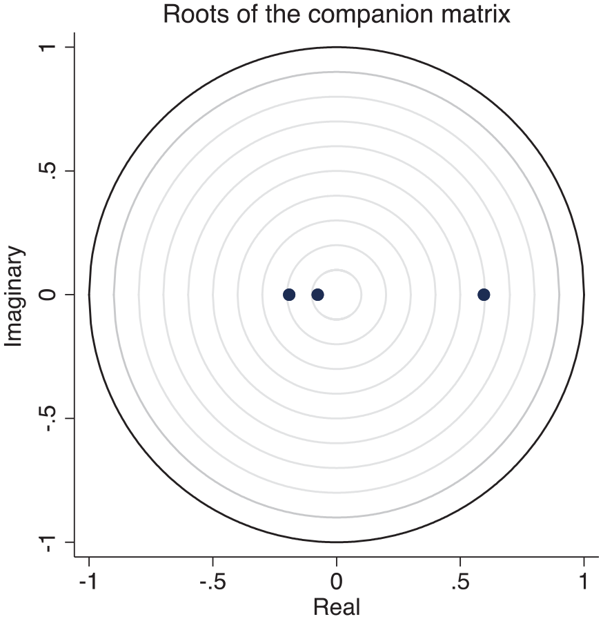
Stability test plot.

Table 6.

Eigenvalue Stability Condition Table.

Eigenvalue		Modulus
Real	Imaginary	Modulus
.595189	0.0000	0.595189
−.1916031	0.0000	0.1916031
−.0761707	0.0000	0.0761707

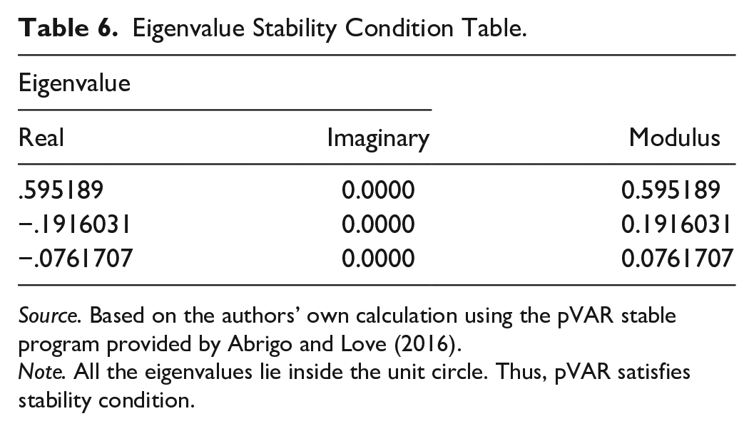
Source. Based on the authors’ own calculation using the pVAR stable program provided by Abrigo and Love (2016).

Note. All the eigenvalues lie inside the unit circle. Thus, pVAR satisfies stability condition.

For the IRFs, we compute the orthogonalised IRF and the cumulative IRF based on Cholesky decomposition. Confidence intervals are computed using 200 Monte Carlo draws on the estimated model. Since the GMM panel VAR is stable, the shocks are expected to converge to zero in the long run. That is, the shocks are anticipated to be temporary, and over the long run, the series are forecasted to return to their deterministic (long-run) trend.

As mentioned, the endogenous variables are ordered as per the Cholesky decomposition. Specifically, we contend, based on intuition, that increase in capital per worker affects output growth contemporaneously, while shocks on the ECI affect output growth with a lag. The result of the Cholesky forecast-error variance decomposition (FEVD) lends support to this ordering, as it shows the impact of the complexity index to be noncontemporaneous while the impact from economic growth on eci is relatively contemporaneous. The result also shows a relatively contemporaneous impact of capital accumulation (investment) on output growth.

Furthermore, given that the contributions of the exogenous variables included in the panel VAR model are disregarded when computing the forecast-error variance, we will only be focusing on the impact of the ECI and the capital accumulation variable on output growth in the rest of the discussion.

The result of the IRF (Figure 3) show the response of economic (output per worker) growth to a shock in eci. The IRF suggest that the eci has a significant impact on economic growth; a 1 standard deviation shock to the ECI at time 0 contributes around 2.34% to the average rate of growth of real GDP per worker within the first period. The point estimates are positive and significant for most horizons up to the 6th period. These results confirm the hypothesis that the ECI is a good predictor of economic growth. The cumulative IRF shows the long-run impact of a standard deviation shock to the ECI on the real output per worker. The result shows that the cumulative increase in the rate of economic growth would be circa 4.4% by the 10th period (Figure 4).

Figure 3.

Response of GDP growth to a shock to economic complexity.

Figure 4.

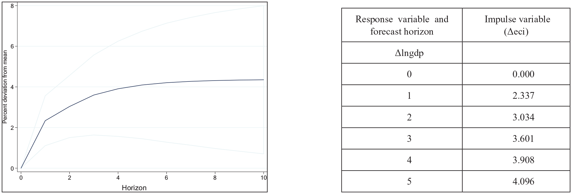
Cumulative response of output growth to a shock to economic complexity.

The effect of capital accumulation on economic growth was also examined. The response of economic growth to a shock in capital per worker is contemporaneous; economic growth reaches a level approximately 1.8 percentage points from the mean in the same period and stays nearly 0.14 percentage points higher up to the fifth period if there is a 1 standard deviation shock to capital per worker (Figure 5).

Figure 5.

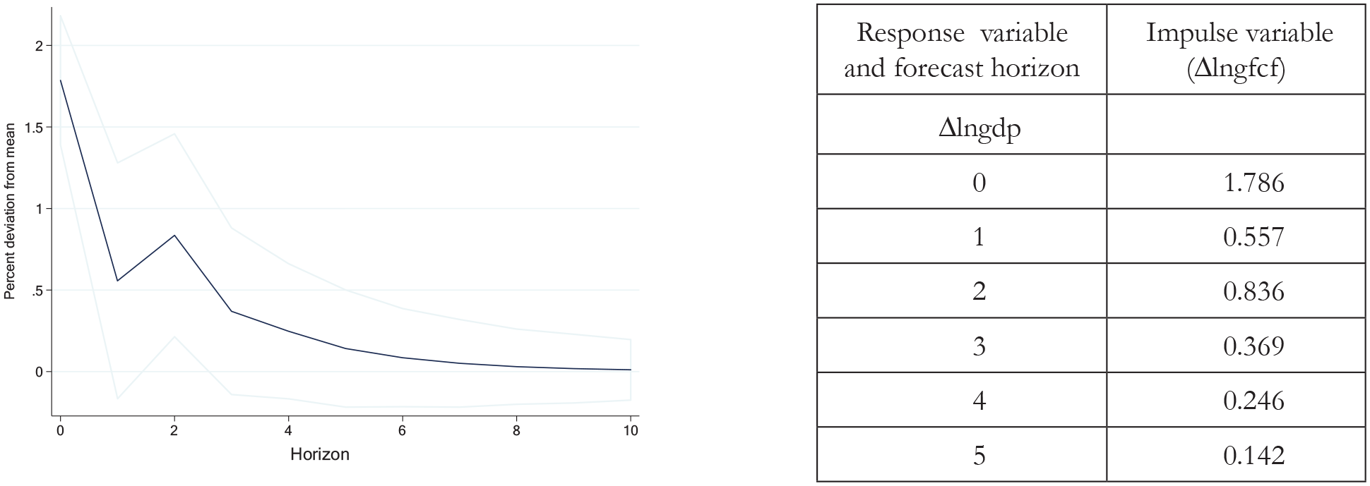
Response of GDP growth to a shock to capital per worker.

Finally, we compared the performance of the ECI to those of the two widely used technical change proxies—the rate of increase in the gross expenditure on research and development (gerd) and the secondary school enrollment (sec) rate. The Granger causality test results for the sec and gerd equations are reported in Tables 7 and 8, respectively. The VAR coefficients are not reported, to save space. From Table 7, we find that the sec term is not statistically different from zero, suggesting that the rate of secondary school enrollment does not Granger cause growth in output per worker. Similarly, results in Table 8 indicate that the rate of gross expenditure on research and development does not Granger cause growth in economic output. These results are undoubtedly plausible, given that not all expenditure on research and development produce significant outputs and likewise increasing secondary school enrollment does not necessarily translate into increasing productivity and output, especially when the quality of the education is not properly accounted for in the enrollment figures.

Table 7.

Granger Test (sec).

Equation	Excluded	Chi-square	df	Prob
∆ lnsec
	∆ lngfcf	0.059	1	.809
	∆ lngdp	4.161	1	.041
	ALL	5.908	2	.052
∆ lngfcf
	∆ lnsec	2.026	1	.155
	∆ lngdp	3.55	1	.06
	ALL	4.657	2	.097
∆ lngdp
	∆ lnsec	0.508	1	.476
	∆ lngfcf	2.821	1	.093
	ALL	2.914	2	.233

Table 8.

Granger Test (Gerd).

Equation	Excluded	Chi-square	df	Prob
∆ lngerd
	∆ lngfcf	0.331	1	.565
	∆ lngdp	1.381	1	.24
	ALL	2.42	2	.298
∆ lngfcf
	∆ lngerd	1.897	1	.168
	∆ lngdp	6.447	1	.011
	ALL	6.784	2	.034
∆ lngdp
	∆ lngerd	0.258	1	.611
	∆ lngfcf	3.982	1	.046
	ALL	4.132	2	.127

Note. Authors’ own estimate. H₀ = excluded variable does not Granger-cause equation variable; H₁ = excluded variable Granger-causes equation variable.

Concluding Remarks

Using data from over 31 OECD countries, covering periods from 1982 to 2017, this study tests the hypothesis that the level of product complexity is a good determinant of economic growth in the long run. The regression is estimated using the generalized method of moment panel vector autoregressive method, which has been shown to be consistent and efficient when endogeneity bias—caused by the omission of relevant variables from a model or an error in the measurement of the variable or due to simultaneous causality between the dependent and independent variable—is present in a model. The paper uses 3-yearly nonoverlapping averages, instead of the annual series, to minimize the impact of short-term shocks. The forward orthogonal transformation is used to control the country effects, and exogenous governance indicators are used to control the effect of factors that change slowly over time, such as the role of law, political stability, regulatory quality, and corruption control.

The results of the empirical analyses show that changes in the level of product complexity and diversity, as measured by the ECI, does indeed determine economic growth in the long run. The IRF shows that a 1 standard deviation shock to the ECI at time 0 contributes around 2.34% to the average rate of growth of real output per worker within the first period. The point estimates are positive and significant for most horizons up to the sixth period. Furthermore, the cumulative IRF shows that the cumulative increase in the rate of economic growth would be around 4.4% by the fifth period.

Compared to traditional technical change proxies such as the gross expenditure on research and development and secondary school enrollment, the ECI performs relatively better in determining economic growth in the long run. The coefficients on both the secondary school enrollment variable and the expenditure on research and development variable appear statistically indifferent from 0 in the empirical result.

Overall, this study offers a substantial quantitative improvement over past studies that have examined the innovation/complexity–growth nexus. The model developed in this article generates dynamics quantitively consistent with several development theories and observations that indicate product complexity and diversity or innovation determines the pace of economic growth cum development in the long run.

The results of this study also contain some policy implications that are certainly noteworthy. The finding is particularly significant for economies both in the OECD and other regions looking for effective ways to stimulate meaningful growth in their economies. The results confirm that by restructuring the economy, particularly by mobilizing resources toward knowledge-intensive manufacturing as well as diversifying exports, countries can stimulate the prerequisite output growth capable of instigating sustainable economic development in the long run. Perhaps the most telling is the confirmation that improving the set of human capital—both the tacit and explicit knowledge, which can be achieved through quality education, nutrition and health care, and investing in physical capital, which includes improvement in available tools and machines and relevant infrastructure (roads, railways, sea and air ports, electricity, internet, etc.), including the enhancement of institutions (economic, political, and social) that exist in a place and time and encourages capital accumulation as well as accelerates economic complexity, are the key engines of growth. This finding helps to take the guesswork away from effective industrial policy design.

Footnotes

Appendix A

Table A1.

Variables Definition and Sources.

Variables	Indicator name	Long definition	Sources
rgdp	GDP (constant 2010 US$)	GDP at purchaser’s prices is the sum of gross value added by all resident producers in the economy plus any product taxes and minus any subsidies not included in the value of the products. It is calculated without making deductions for depreciation of fabricated assets or for depletion and degradation of natural resources. Data are in constant 2010 U.S. dollars. Dollar figures for GDP are converted from domestic currencies using 2010 official exchange rates. For a few countries where the official exchange rate does not reflect the rate effectively applied to actual foreign exchange transactions, an alternative conversion factor is used.	OECD National Accounts data files, https://data.oecd.org
gfcf	Gross-fixed capital formation (constant 2010 US$)	Gross-fixed capital formation (formerly gross domestic investment) consists of outlays on additions to the fixed assets of the economy plus net changes in the level of inventories. Fixed assets include land improvements (fences, ditches, drains, and so on); plant, machinery, and equipment purchase; and the construction of roads, railways, and the like, including schools, offices, hospitals, private residential dwellings, and commercial and industrial buildings. Inventories are stocks of goods held by firms to meet temporary or unexpected fluctuations in production or sales, and “work in progress.” This is according to the 1993 SNA; net acquisitions of valuables are also considered capital formation. Data are in constant 2010 U.S. dollars.	OECD National Accounts data files, https://data.oecd.org
eci	Economic complexity index	ECI is derived from the method of reflections of Hidalgo and Hausmann (2009). The index combines information on the diversity of a country (the number of products it exports), and the ubiquity of its products (the number of countries that export that product) to reflect the diversity and complexity of capabilities (that is, the knowledge, know-how, social capital, institutions, etc.) available in a country and their interactions.	“The Atlas of Economic Complexity,” Center for International Development at Harvard University, http://www.atlas.cid.harvard.edu.
polstab	Political stability and absence of violence/terrorism: estimate	Political stability and absence of violence/terrorism measures perceptions of the likelihood of political instability and/or politically motivated violence, including terrorism. Estimate gives the country’s score on the aggregate indicator, in units of a standard normal distribution, that is, ranging from approximately −2.5 to 2.5.	The World Bank’s WGI database, https://databank.worldbank.org/source/worldwide-governance-indicators
regq	Regulatory quality: estimate	Regulatory quality captures perceptions of the ability of the government to formulate and implement sound policies and regulations that permit and promote private sector development. Estimate gives the country’s score on the aggregate indicator, in units of a standard normal distribution, that is, ranging from approximately −2.5 to 2.5.	The World Bank’s WGI database, https://databank.worldbank.org/source/worldwide-governance-indicators
rule	Rule of law	Rule of law captures perceptions of the extent to which agents have confidence in and abide by the rules of society, and in particular the quality of contract enforcement, property rights, the police, and the courts, as well as the likelihood of crime and violence. Estimate gives the country’s score on the aggregate indicator, in units of a standard normal distribution, that is ranging from approximately −2.5 to 2.5.	The World Bank’s WGI database, https://databank.worldbank.org/source/worldwide-governance-indicators
Coc	Control of corruption	Control of corruption captures perceptions of the extent to which public power is exercised for private gain, including both petty and grand forms of corruption, as well as “capture” of the state by elites and private interests. Estimate gives the country’s score on the aggregate indicator, in units of a standard normal distribution, that is ranging from approximately −2.5 to 2.5.	World Bank’s WGI database, https://databank.worldbank.org/source/worldwide-governance-indicators

Note. GDP = gross domestic product; OECD = Organization for Economic Co-operation and Development; ECI = Economic Complexity Index; WGI = World Governance Indicator.

Appendix B

Appendix C

The Breusch and Pagan (1980) proposed that Lagrange multiplier (LM) test is used to test the presence of panel effect in the model—that is, whether there is significant differences across the units. The null hypothesis of the LM test is that variances across the entities is zero. So, the failure to reject the null hypothesis means the OLS would be a more appropriate estimator to use. The Pesaran (2007) test is used to assess whether there is a contemporaneous correlation among the residuals. One of the assumptions of the GMM model is that there is no cross-sectional dependence. The null of the Pesaran cross-section dependence (CD) test is that residuals are not correlated. To be consistent, we would expect to accept the null of the Pesaran CD test. To test for homoskedasticity or constant variance, we applied the modified Wald test for groupwise heteroskedasticity. In a fixed-effect regression model, the test has a null of homoskedasticity or constant variance. Results of these preliminary tests show that the use of the GMM pVAR is relevant and appropriate in this context, given the presence of individual effects and cross-sectional independence. The presence of heteroskedasticity in the model requires the use of robust standard errors, which we applied in the main model accordingly.

Appendix D

Appendix E

Availability of Data and Material

The datasets used and/or analyzed during the current study are available from the corresponding author on reasonable request.

Declaration of Conflicting Interests

The author(s) declared no potential conflicts of interest with respect to the research, authorship, and/or publication of this article.

Funding

The author(s) received no financial support for the research, authorship, and/or publication of this article.

ORCID iDs

Ejike Udeogu

Uzochukwu Amakom

References

Abdon

Felipe

(2011). The product space: What does it say about the opportunities for growth and structural transformation of Sub-saharan Africa? (Levy Economics Institute Working Paper Archive No, wp_670). https://ideas.repec.org/p/lev/wrkpap/wp_670.html

Abrigo

M. R. M.

Love

(2016). Estimation of panel vector autoregression in stata. Stata Journal, 16(3), 778–804.

Acemoglu

Gallego

F. A.

Robinson

J. A.

(2014). Institutions, human capital, and development. Annual Review of Economics, 6(1), 875–912.

Acemoglu

Naidu

Restrepo

Robinson

J. A.

(2019). Democracy does cause growth. Journal of Political Economy, 127(1), 47–100.

Acemoglu

Robinson

(2012). Why nations fail: The origins of power, prosperity, and poverty. Crown.

Aghion

Howitt

(1992). A model of growth through creative destruction. Econometrica, 60, 323–351.

Aghion

Howitt

(1998a). Capital accumulation and innovation as complementary factors in long-run growth. Journal of Economic Growth, 3, 111–130.

Aghion

Howitt

(1998b). Endogenous growth theory. MIT Press.

Akaike

(1969). Fitting Autoregressive Models for Prediction. Annals of the Institute of Statistical Mathematics, 21, 243–247. https://doi.org/10.1007/BF02532251

10.

Akaike

(1977). Likelihood of a model and information criteria, Journal of Econometrics, 16(1), 3–14.

11.

Anderson

T. W.

Hsiao

(1982). Formulation and estimation of dynamic models using panel data. Journal of Econometrics, 18(1), 47–82.

12.

Andrews

D. W. K.

(2001). Consistent model and moment selection procedures for GMM estimation with application to dynamic panel data models. Journal of Econometrics, 101(1), 123–164.

13.

Arellano

Bond

(1991). Some tests of specification for panel data: Monte Carlo evidence and an application to employment equations. Review of Economic Studies, 58, 277–297.

14.

Arellano

Bover

(1995). Another look at the instrumental variable estimation of error-components models. Journal of Econometrics, 68, 29–51.

15.

Baltagi

B. H.

(2013). Econometric analysis of panel data. John Wiley.

16.

Barro

(1991). Economic growth in a cross section of countries. Quarterly Journal of Economics, 106(2), 407–443.

17.

Barro

(1997). Determinants of economic growth: A cross-country empirical study. MIT Press.

18.

Barro

(2001). Human capital and growth. American Economic Review, 91(2), 12–17.

19.

Barro

Chu

Cozzi

(2017). Intermediate macroeconomics. Cengage.

20.

Bilbao-Osorio

Rodríguez-Pose

(2004). From R&D to innovation and economic growth in the EU. Growth and Change, 35, 434–455.

21.

Blomquist

WesterLund

(2013). Testing slope homogeneity in large panels with serial correlation. Economic Letters, 121(3), 374–378.

22.

Blundell

Bond

(1998). Initial conditions and moment restrictions in dynamic panel data models. Journal of Econometrics, 87, 115–143.

23.

Blundell

Bond

(2000). GMM estimation with persistent panel data: An application to production functions. Econometric Reviews, 19(3), 321–340.

24.

Bond

Leblebicioglu

Schiantarelli

(2010). Capital accumulation and growth: A new look at the empirical evidence. Journal of Applied Econometrics, 25(7), 1073–1099.

25.

Breusch

T. S.

Pagan

A. R.

(1980). The lagrange multiplier test and its applications to model specification in econometrics. The Review of Economic Studies, 47(1), 239–253.

26.

Caldarelli

Cristelli

Gabrielli

Pietronero

Scala

Tacchella

(2012). A network analysis of countries’ export flows: Firm grounds for the building blocks of the economy. PLoS ONE, 7(10), Article e47278.

27.

Carpenter

Demiralp

(2012). Money, reserves, and the transmission of monetary policy: Does the money multiplier exist? Journal of Macroeconomics, 34, 59–75.

28.

Coe

D. T.

Helpman

(1995). International R&D spillovers. European Economic Review, 39(5), 859–887.

29.

Cristelli

Tacchella

Pietronero

(2015). The heterogenous dynamics of economic complexity. PLoS ONE, 10(2), Article e0117174.

30.

Dos Santos

. (1970). The structure of dependence. American Economic Review, 60(2), 231–236.

31.

Frank

(1967). Capitalism and underdevelopment in Latin America. Monthly Review Press.

32.

Griliches

(1994). Productivity, R&D, and the data constraint. American Economic Review, 84, 1–23.

33.

Griliches

(1998). R&D and productivity: The econometric evidence. University of Chicago Press.

34.

Griliches

Mairesse

. (1990). R&D and productivity growth: Comparing Japanese and U.S. manufacturing firms. In Hulten

C. R.

(Ed.), Productivity growth in Japan and the United States (pp. 317–348). Chicago University Press. https://doi.org/10.7208/9780226360607-014

35.

Grossman

G. M.

Helpman

(1991a). Innovation and growth in the global economy. MIT Press.

36.

Grossman

G. M.

Helpman

(1991b). Trade, knowledge spillovers, and growth. European Economic Review, 35, 517–526.

37.

Grossman

G. M.

Helpman

(1994). Endogenous innovation in the theory of growth. Journal of Economic Perspectives, 8(1), 23–44.

38.

Guellec

Potterie

(2003). The impact of public R&D expenditure on business R&D. Economics of Innovation and New Technology, 12, 225–243.

39.

Hall

B. H.

Mairesse

Mohnen

(2010). Measuring the returns to R&D. In Hall

H. B.

Rosenberg

(Eds.), Handbook of the economics of innovation (Vol. 2., pp. 1033–1082). Elsevier.

40.

Hannan

E. J.

Ouinn

B. G.

(1979). The determination of the order of an autoregression. Journal of the Royal Statistical Society: Series B (Methodological), 41(2), 190–195.

41.

Hansen

E. B.

(2018). Econometrics. University of Wisconsin.

42.

Hamilton

J. D.

(1994). Time series analysis. Princeton University Press.

43.

Hartmann

Guevara

R. M.

Jara-Figueroa

Aristaran

Hidalgo

A. C.

(2017). Linking economic complexity, institutions, and income inequality. World Development, 93, 75–93.

44.

Hausmann

Hidalgo

C. A.

Bustos

Coscia

Chung

Jimenez

Simoes

Yildirim

(2014). The atlas of economic complexity. Puritan Press.

45.

Head

Lloyd-Ellis

Sun

(2016). Search, liquidity, and the dynamics of house prices and construction. American Economic Review, 106, 1214–1219.

46.

Hidalgo

C. A.

Hausmann

(2009). The building blocks of economic complexity. Proceedings of the National Academy of Sciences, 106(26), 10570–10575.

47.

Hirschman

A. O.

(1958). The strategy of economic development. Yale University Press.

48.

Jones

(1995). Time series tests of endogenous growth models. The Quarterly Journal of Economics, 110, 495–525.

49.

Kemeny

Storper

(2014). Is specialization good for regional economic development? Regional Studies, 49(6), 1003–1018.

50.

Kotz

D. M.

McDonough

Reich

(1994). Social structures of accumulation: The political economy of growth and crisis. Cambridge University Press.

51.

Levine

Loayza

Beck

(2000). Financial intermediation and growth: Causality and causes. Journal of Monetary Economics, 46(1), 31–77.

52.

Lewis

W. A.

(1954). Economic development with unlimited supplies of labour. The Manchester School, 22(2), 139–191.

53.

Lucas

R. E.

(1988). On the mechanics of economic development. Journal of Monetary Economics, 22, 3–42.

54.

Lutkepohl

(2005). New introduction to multiple time series analysis. Springer.

55.

Mankiw

N. G.

Romer

Weil

D. N.

(1992). A contribution to the empirics of economic growth. The Quarterly Journal of Economics, 107(2), 407–437.

56.

Mohnen

(1990). New technologies and inter-industry spillovers. STI Review, (OECD), 131–147.

57.

Mohnen

Lépine

(1991). R&D, R&D spillovers and payments for technology: Canadian evidence. Structural Change and Economic Dynamics, 2, 213–228.

58.

Mora

Logan

(2012). Shocks to Bank Capital: Evidence from UK Banks at Home and Away. Applied Economics, 44, 1103–1119.

59.

Neumann

T. C.

Fishback

P. V.

Kantor

(2010). The dynamics of relief spending and the private urban labour market during the new deal. Journal of Economic History, 70, 195–220.

60.

Pesaran

M. H.

(2007). A simple panel unit root test in the presence of cross-section dependence. Journal of Applied Econometrics, 22(2), 265–312.

61.

Pesaran

M. H.

Smith

(1995). Estimating long-run relationships from dynamic heterogenous panels. Journal of Econometrics, 68(1), 79–113.

62.

Pesaran

M. H.

Yamagata

(2008). Testing slope homogeneity in large panels. Journal of Econometrics, 142(1), 50–93.

63.

Prebisch

(1963). Towards a dynamic development policy for Latin America. United Nations.

64.

Rebelo

(1991). Long-run policy analysis and long-run growth. Journal of Political Economy, 99, 500–521.

65.

Romer

P. M.

(1986). Increasing returns and long-run growth. Journal of Political Economy, 94, 1002–1037.

66.

Romer

P. M.

(1987). Growth based on increasing returns due to specialization. American Economic Review, 77, 56–62.

67.

Romer

P. M.

(1990). Endogenous technological change. Journal of Political Economy, 98, 71–102.

68.

Roodman

(2009). How to do xtabond2: An introduction to difference and system GMM in Stata. Stata Journal, 9(1), 86–136.

69.

Rosenstein-Rodan

P. N.

(1943). Problems of industrialisation of eastern and south-eastern europe. The Economic Journal, 53(210/211), 202–211.

70.

Schwarz

(1978). The Annals of Statistics, 6(2), 461–464.

71.

Singer

H. W.

(1950). The distribution of gains between investing and borrowing countries. American Economic Review, 40(2), 473–485.

72.

Solow

R. M.

(1956). A contribution to the theory of economic growth. The Quarterly Journal of Economics, 70(1), 65–94.

73.

Solow

R. M.

(1957). Technical change and the aggregate production function. The Review of Economics and Statistics, 39, 312–320.

74.

Wallerstein

(2004). World-systems analysis: An introduction. Duke University Press.

75.

Williamson

J. G.

(2013). Trade and poverty: When the third world fell behind. MIT Press.

76.

Zachariadis

(2003). R&D, innovation, and technological progress: A test of the schumpeterian framework without scale effects. Canadian Journal of Economics, 36(3), 566–586.

Does Increasing Product Complexity and Diversity Cause Economic Growth in the Long-Run? A GMM Panel VAR Evidence

Abstract

Keywords

Introduction

Conceptual Framework

Data Sources, Variables Description, and Empirical Method

Discussion of Results

Concluding Remarks

Footnotes

Appendix A

Appendix B

Appendix C

Appendix D

Appendix E

Availability of Data and Material

Declaration of Conflicting Interests

Funding

ORCID iDs

References