Displacement Effect and Ratchet Effect: Testing of Two Alternative Hypotheses

Abstract

This article empirically tests the displacement effect of Peacock and Wiseman (PW) and the ratchet effect of Bird, both of which are alternatives to Wagner’s law on the growth of public expenditure. The displacement effect explains why the (horizontal) trend line moves upward in discrete steps over time, whereas the ratchet effect affirms that public expenditure “ratchets” during drops in the economy and remains at a higher level after the economy stabilizes. The following innovations are introduced in the present study: (a) empirical testing was conducted for Spain and an extensive time period, 1880–2016; (b) the relationship between PR and expenditure was considered, introducing Gross Domestic Product (GDP) as a control variable; and (c) testing was performed using two differentiated methodologies. More specifically, the two methodologies employed were unit roots and cointegration with structural breakpoints and the more recent wavelet methodology. Given that PW refer to situations of social upheaval and its consequences, this study places its focus on analyzing the changes produced in Spain’s public expenditure with respect to the Spanish Civil War of 1936–1939 and to other disruptions both before and after this date. It was concluded that the displacement effect explains the development of Spanish public expenditure for the crises of 1982 and 1998. Meanwhile, wavelet methodology explains growth that took place in 1920 and 1980. In contrast, the ratchet effect does not explain the development of Spanish public expenditure over the study period.

Introduction

The displacement effect hypothesis was presented by Peacock and Wiseman (PW) in their 1961 monograph “The Growth of Public Expenditure in the United Kingdom.” According to this hypothesis, government spending tends to increase in a staggered manner, coinciding with social disturbances, particularly wars.

In addition to analyzing the displacement effect, the present work studies the ratchet effect as applied to public expenditure. This theory was formulated by Bird (1972), who considered PW’s theory to be unconvincing, prompting the author to create his own alternative.

The ratchet effect, as applied to government growth, maintains the hypothesis that temporary crises cause public expenditure to rise and permanently remain higher than it would have been had said crises not occurred.

As for the displacement effect, its scope will be greater if there is a ratchet effect as well. The displacement effect results from divergent opinions regarding the size of the public sector: Whereas bureaucrats and politicians are in favor of a larger public sector, citizens/taxpayers are not willing to finance greater levels of public expenditure. While the public sector grows consistently in periods of normality, resistance to taxes decreases, yet the size of the public sector tends to increase during wars or economic crises. During such periods, public expenditure tends to exceed what would have been normal previously. Wars and depressions have a displacement effect on the size of the public sector. Consequently, political leaders use national crises to increase the equilibrium level between public revenue (PR) and spending.

Both hypotheses are proposed as alternatives to Wagner’s law. PW found Wagner’s law to be an unconvincing explanation for growth in public expenditure (PE), which led them to formulate the displacement effect hypothesis. PW did not find Wagner’s historical determinism appropriate and believed it necessary to reject the corresponding predictive arguments. Meanwhile, Bird adapted the ratchet effect hypothesis as an alternative to the displacement effect and, in turn, as an alternative to Wagner’s law.

The present study empirically tests the two theories using public expenditure data from Spain for the period 1880–2016. Compared with prior works, the following innovations are introduced: (a) empirical testing was conducted for Spain and an extensive time period, 1880–2016; (b) the relationship between PR and spending was considered, introducing Gross Domestic Product (GDP) as a control variable; and (c) testing was performed using two differentiated methodologies. More specifically, the two methodologies employed were unit roots and cointegration with structural breakpoints and the more recent wavelet methodology.

Initially, the Spanish Civil War will be considered in the first section, along with other social disturbances that occurred both before and after. “Displacement Effect and Ratchet Effect” section briefly analyzes both theories. “Literature Review” section reviews the empirical works that test both theories. “Empirical Testing of the Spanish Case” and “An Alternative Explanation of the Displacement Effect Using Wavelet Methodology” sections test these theories specifically with respect to Spain, using unit root and cointegration methodology and wavelet methodology, respectively. “Conclusion” section summarizes this work and presents the conclusions.

Displacement Effect and Ratchet Effect

PW demonstrated that while PE grew over time relative to the rest of the economy, the growth pattern was not as uniform as was required by Wagner’s law. This law states that public expenditure growth is absolute and relative within the national economy, in particular for government services destined for public purposes, at the expense of the private sector. The growth path may be different for the various branches of government but would always include the traditional services, such as defense, law and order, and the development of new functions associated with expansion of education, health care services, and structural changes in the economy (Adil et al., 2017; Forte & Magazzino, 2018; Magazzino, 2012a, 2012b; Magazzino et al., 2015; Peacock & Scott, 2000).

For PW, foreign wars and other social disturbances abruptly resulted in increased PE in Great Britain. As permanent factors could not support the model of PE, which graphically took the form of a ladder, Wagner’s law became obsolete. The displacement effect theory arose when PW sought to explain irregular growth in PE in Great Britain. They distanced themselves from Wagner’s law on two points: (a) rather than analyze the long-term increase of PE, they focused on the more immediate pattern of that growth; and (b) unlike Wagner, they did not adopt any general theory of the State, although they did have to make three politically oriented assumptions: (a) rulers always want to spend more money; (b) taxpayers never want to pay more taxes; and (c) to some degree, rulers must depend on the wishes of their citizens (Comín, 1985; Henrekson, 1990, 1993; Peacock & Wiseman, 1961/1967).

PW’s analysis focuses on explaining the temporary behavior of PE growth, rather than on considering the absolute magnitude of said value. In other words, it addresses how public expenditure can vary according to given behavioral hypotheses. In their study of the period 1890–1955, they observed that government expenditure grew not at a steady rate, but rather in a staggered manner. PW found that so-called permanent impacts on growth, such as population and employment trends, were not useful for explaining the observed short-term behavior; thus, they considered other influences to be more relevant. The explanation that these authors propose rests on rudimentary theories of political process and social disturbance (in the introduction, Peacock & Wiseman, 1961/1967). As there is no direct mechanism of choice in the political marketplace as there is in the social market, citizens who vote for goods to be supplied to their community have different ideas relating to the desirable level of spending and the “tolerable” tax burden that must be imposed on them or on particular social groups. As a result of this political struggle, the views of voters can differ significantly regarding who will or should bear the burden of providing public services and who will benefit at the expense of others, at least partially.

During “normal” times, the existence of a general notion of “tolerable burden” is likely to restrict the pattern of practical implementation of public expenditure plans. However, if this restriction is weakened or destroyed during periods of social disturbance, which is when these notions of taxation are most easily dismantled, then the gap between desirable growth of public expenditure and a “tolerable” tax burden may narrow. The process is complex, although it seems to have some permanent characteristics. After a disturbance, the tolerable rates of taxation do not return to their original levels, allowing the government to implement spending programs that it had been previously desired, but which could not be financed. However, once the displacement effect raises spending above its previous level, the new tolerable tax burden remains unchanged, preventing a growth in public expenditure until there is a new social disturbance (Peacock & Wiseman, 1961/1967).

Therefore, PW proceeded to examine the extent to which spending growth could be explained simply as the direct and inevitable consequence of war. This led them to formulate the hypothesis of the “displacement effect.” They affirm that their theory is not ordered or carefully planned, nor can it be expressed as a set of equations that forms a system that can be used for predictive or empirically testable purposes.

In addition to the displacement effect, they highlight the “inspection effect” of wars. During periods of war, the allocation of human resources to certain purposes may incidentally reveal previously unavailable information regarding social or other conditions; this new knowledge may move public opinion in favor of new and increased public expenditure of certain types after a return to normality. At the same time, governments consider themselves capable of implementing new policies with relative ease, as the disturbance itself makes it possible to broaden the tax base, which temporarily weakens the “tolerable burden” restriction, accustoming citizens to a new and higher level of taxes. This process explains the short-term trajectory of public expenditure that occurs after the social disturbance recedes.

PW identify a third influence called the “concentration process” (Rowley & Tollison, 1994), which is related to the changes in accountability regarding public expenditure. They state that periods of displacement lower the barriers that protect local authorities and create pressure to concentrate power over public expenditure within the central government. This concept is distinct from the displacement effect in that the forces favoring centralization operate during both normal and disruptive times. However, periods of displacement are considered particularly important when considering the process of centralizing public expenditure.

To summarize, the displacement effect explains why the (horizontal) trend line moves upward in discrete steps over time. In this sense, it serves as a theory of long-term government spending behavior comparable with Wagner’s law (Rosenfeld, 1973). PW propose that “the tolerable tax burden” is the driving force behind the displacement effect. Unfortunately, it is not clear how this concept can be defined, although most authors understand it to be a tolerable or reasonable tax rate (Henrekson, 1990, 1993; Rowley & Tollison, 1994). On the contrary, there is also evidence that the absolute levels of per capita spending are sometimes considered in the literature.

Based on the previous review of the original hypothesis, the following two testable versions of the displacement effect hypothesis can be deduced:

• Hypothesis 1: Absolute real public expenditure per capita evolves in a stepwise manner, featuring steps coinciding with important social disturbances, such as wars.

• Hypothesis 2: The ratio of PE to GDP (PE/GDP) evolves in the same manner.

A third version can be attributed to Gupta (1967), who was the first to econometrically test the hypothesis, expanding on PW’s concept in the sense that it should examine whether a disturbance is associated with a change in the rate of growth of government spending with respect to economic growth.

The ratchet effect in this context originated with Duesenberry (1949), who used it to explain short-term changes in the ratio between consumption and income over time. Bird (1972) shows that it can be used as a displacement effect alternative, in line with the study of the consumption function. Bird provides the following figures to explain his theory.

In Figure 1A, the ratio of government expenditure to GDP, G/Y, moves along the trajectory represented by OB in the long term, indicating the applicability of Wagner’s law. The “pure” displacement effect describes upward displacement in tax burden over time, produced by the crisis that causes a movement along OB, from R to S. Alternatively, the ratchet effect posits that the ratio G/Y increases over time along OB, but that it does not decrease along that trajectory. During crises, if per capita income drops, G also falls, but less quickly due to administrative inertia in adjusting spending plans; therefore, the ratio G/Y increases along the length of the curve in the short-term GG (Figure 1B). The pure ratchet effect describes cyclic movements in the ratio G/Y around an upward tendency over the long term. Given that the displacement effect describes displacement as always increasing the spending ratio, the increase in the ratio G/Y described by the function in the short term is eventually reconciled with the function OB in the long term via upward displacements in taxation as the result of a crisis, in other words, displacements from the short-term function GG to G′G′.

Figure 1.

(A) Displacement effect (B) Ratchet effect.

According to Bird (1972), the current ratio G/Y can fall over the length of a line such as OB. OB illustrates Wagner’s law, with time as a third, implicit dimension in the figure. The pure displacement hypothesis is that the tolerable tax burden displaces upward over time as the result of a crisis (e.g., from TT to T′T′). In addition, given that revenue in the long term should be equal to expenditure, it is the change that allows movement along OB from R to S. Essentially, without a crisis that enables increased taxes, this movement would not be produced. The ratchet hypothesis is illustrated in the second figure, in which OB is the new public expenditure function over the long term. The course of public expenditure in the long term can be described in the following manner: Under normal conditions, when income per capita increases, the ratio of public expenditure (G/Y) moves along OB, specifically, from R to S. If there is a crisis and income per capita decreases, such as in a depression, G decreases as well, but less quickly, meaning that G/Y increases, but over the length of the curve GG instead of that of OB. These short-term curves are drawn to reflect the fact that spending does not fall as rapidly as income, meaning that the ratio G/Y increases. If income does not fall, but rather increases during a crisis, then the spending ratio will also increase, but more slowly at the beginning, given that it takes time to adjust spending (e.g., over the length of G′). Afterward, the value increases more rapidly, more precisely, when spending and the political realities move the economy again to OB, the curve which describes the desired level of spending at each level of income (and, in this analysis, when there is no restriction on revenue in the long term, achieved level of spending). The speed at which this adjustment takes place is reflected in the income elasticity of public expenditure, which, as expected, varies considerably depending on how much time has passed since the last crisis. However, it is likely statistically impossible to distinguish this factor, given the confusion inherent in the slope of OB and the influence of the other two factors (income elasticity and budget process).

The true virtue of the ratchet effect is the fact that it is firmly based on the common belief regarding the way in which PE enters the function of individual preference on consumer behavior theory regarding the relative permanence of variables that determine individuals’ tastes during a temporary crisis.

Certainly, what Bird postulates is an asymmetric response on the part of public-sector expansion to changes in income. In accordance with the ratchet hypothesis, the change in the expected value of public expenditure in response to a unitary increase in income per capita is different in absolute value from a unitary decrease in income per capita (that is to say, public expenditure will hardly decrease). The displacement effect only considers the temporary trajectory of public expenditure and does not concern itself with the reasons why there is constant pressure (assuming there is), which causes the ratio of public expenditure to increase over time.

In an operational and empirically testable way, the ratchet effect affirms that for an economy in recession, public expenditure decreases more slowly than per capita income, thereby increasing the ratio of public expenditure to GDP. Inversely, in periods of growth, public expenditure increases more slowly than per capita income and, consequently, the ratio of public expenditure to income decreases. Public expenditure “ratchets” during drops in the economy and remains at a higher level after the economy stabilizes.

Literature Review

Unlike Wagner’s law, which has received significant empirical attention, the displacement effect and the ratchet effect have been tested sporadically.

After formulating their theoretical model to run counter to Wagner’s law, Peacock and Wiseman performed their analysis based on figures of the total expenditure of the government of Great Britain and those components corresponding to defense and war; these were set in absolute terms, with respect to GDP and per capita, using the national currency adjusted for inflation to its value in 1900. Their goal was to confirm that the resulting profile would continue to evolve in a stepwise manner once the factors that act permanently on PE were removed. With this correction, the displacement effect in Great Britain remained so evident through the two world wars that the use of econometric testing for the same purpose was deemed a waste of time.

As PW affirm, their theory is not ordered or carefully planned, nor can it be expressed as a set of equations that forms a given system that can be used for predictive or empirically testable purposes. It is precisely this nature of the theory that has allowed the numerous and various interpretations that have been produced over time. For example, Gupta (1967) considers not just the displacement produced on the level of government spending with respect to economic growth but also the change in “income elasticity” of government spending (using the term to express the rate of growth of government spending per capita with respect to that of income per capita). Meanwhile, Pryor (1968) adapts a dummy variable technique, considering a relation between public expenditure and time. Bonin et al. (1969) try to include a displacement effect, arguing that displacements in public expenditure produced by war persist after hostilities end, given the need to use them to cover peace-time expenditures, such that 100% of the nonmilitary sacrifices during war time are replaced in the immediate postwar years. Furthermore, Diamond (1977) reinterpreted the displacement effect as a theory of structural breakpoints. Peacock and Wiseman (1979) subscribe to this reinterpretation in an article reviewing different approaches to analyzing growth in government spending. Andre and Delorme (1978) consider that a rigorous testing of the displacement effect, which they call the threshold effect, requires empirical analysis of the tax burden, the stability of the ratio of PE/GDP, and the jumps, based on clear theoretical specifications. According to O’Hagan (1980), Irish public expenditure is related to that of Great Britain, which leads to the inclusion of what is called a demonstration effect to present the association of spending tendencies between both countries.

Henrekson (1990, 1993) considers three possible versions of the displacement hypothesis:

• Hypothesis 1: The strong version: Absolute real government spending per capita evolves in a stepwise manner, with steps coinciding with important social disturbances, such as wars.

• Hypothesis 2: The semi-strong version: Government spending as a proportion of national income evolves in the same manner.

• Hypothesis 3: The weak version: The ratio of government spending to GDP trends upward under normal circumstances. This tendency shifts permanently upward after a social disturbance.

Through empirical testing, these three versions were rejected for both Great Britain and Sweden.

Nomura (1995) examines the displacement effect resulting from the first and second petroleum crises on government expenditure in Japan. Goff (1998) interprets the displacement effect as an impulse response in an autoregressive–moving-average model of the first difference in the series of public expenditure in absolute terms and with respect to GDP. Legrenzi (2004), following Ashworth (1995), estimates an error correction model that includes as independent variables tax revenues, both in absolute terms and with respect to GDP, the population, and both GDP and PE. The two world wars are considered dummy variables. Durevall and Henrekson (2011) interpret the displacement effect in such a way that public expenditure resembles a series of plateaus separated by peaks; these peaks coincide with periods of war and preparation for war. The displacement effect affirms that the (horizontal) trend line moves upward in discrete steps over time, such that any temporary shock to public expenditure can have a permanent or highly persistent effect. These changes are infrequent but very large. Henry and Olekalns (2010) claim that they tested the displacement effect, although, in fact, they limited themselves to confirming that there are structural breaks in public expenditure, using a Bai–Perron structural breakpoint test. Carter (2012) interprets the displacement effect in the context of war between states. This analysis considers the increase in tax revenue and military and social spending in 52 states and analyzes whether these variations are produced by a displacement effect. Ageli (2013) tests what is called the PW version of the displacement effect hypothesis for Saudi Arabia. Funashima (2017) tests the displacement effect in a wavelet context. According to this study, when a significant region of the public expenditure variable spectrum coincides with the region of coherence between public expenditure and GDP, long-term growth of PE/GDP is due to Wagner’s law. Alternatively, when frequencies in the significant region of the public expenditure variable spectrum are lower than those for which Wagner’s law is valid, the displacement effect can explain a large part of the growth in PE/GDP.

Comín (1985) and Jaén-García (1998) have conducted testing in the case of Spain. The former applies the procedure proposed by Gupta to estimation by ordinary least squares (OLS), finding that none of the three social disturbances (both world wars and the stock market crash of 1929) encompass PW’s theory. The dummy variable method (Bonin et al., 1969; Pryor, 1968) also yields unfavorable results for PW’s theory. Upon using the Chow test, precisely as Diamond did, it is shown that all tested Spanish disturbances resulted in structural breakpoints in the function of spending by the State, specifically total and nonmilitary spending. Jaén-García considers the displacement effect over the period of 1901–1992, during which the Spanish Civil War is the event that could have provoked a displacement in public expenditure. Using Henrekson’s three versions, it was concluded that there is an upward displacement in the ordinate at the origin in the third version. As the coefficient corresponding to the PW dummy variable is negative (PW = 1 from 1940 onward and 0 otherwise), the Spanish Civil War is shown to have decreased both the PE/GDP ratio and spending per capita.

As for the ratchet effect, very limited testing has been conducted with this theory. Diamond (1977) considers that the change in the expected value of public expenditure in response to a unitary change in income per capita is different in absolute value from a unitary decrease in income per capita (meaning public expenditure will hardly decrease). Goff (1998) tested the displacement effect in a manner that Durevall and Henrekson considered a test of the ratchet effect. Hercowitz and Strawczynski (2004) consider the role of business cycles in the increasing ratios of PE/GDP in Organisation for Economic Co-operation and Development (OECD) countries for the period of 1975–1998. Durevall and Henrekson (2011) analyze the ratchet effect considering that economic recessions tend to affect the ratio PE/GDP, leading to a ratchet effect. Grenade and Wright (2014) aim to determine the asymmetric nature of public expenditure in response to economic cycles when testing the ratchet hypothesis.

Empirical Testing of the Spanish Case

As has been discussed in the previous sections, PW originally considered the theoretical explanation of the displacement effect in terms of a simple fiscal decision-making process. This perception considered that the influences of supply—the ease with which the government can increase revenues—exercise as much influence on the growth of public expenditure as the demand for public services. Their presentation focuses on the forces that push for increasing public services and the restrictions they face in obtaining the necessary revenue. In particular, they highlight the idea that the government views the electorate as having some level of imposition that is seen as “tolerable.” Although the displacement effect should be explained in terms of the fiscal decision-making process, econometric testing has tended to ignore the supply side. In econometric studies, causal interpretations represent the dominant method used by authors. First, an exogenous factor disrupts the normal relationship between public expenditure and national income causing it to move upward; tests have considered the significance of these shifts. Second, the displacement effect has been interpreted as a change in the behavior that dictates the size of the public sector before and after exogenous shocks such as wars. In all studies, income per capita is chosen as a strategic variable and a coefficient of elasticity is calculated; as such, there is a tendency to minimize supply influences.

In our interpretation of the displacement effect, we consider these supply factors as represented by the level of tolerable tax burden, along with the influence of economic growth. In other words, we consider fiscal revenue to be an independent variable. We take the econometric properties of the selected time series as variables: Public expenditure and revenue, as well as economic growth, represented by GDP per capita. We analyze whether the variables are stationary and, in the event that it is not, whether its order of integration is I(1) or higher. If it is I(1), we know that estimating the corresponding equation or equations via OLS would be invalid, meaning we determine whether the set is cointegrated. In the event that it is, we estimate the corresponding cointegration equation using Fully Modified OLS (FMOLS).

We begin the analysis by studying the evolution of the three variables mentioned: PE, PR, and GDP.

Tables 1 and 2 and Figure 2 display the descriptive statistics, the correlation between the variables, and their evolution. Table 1 shows the difference between the maximum and the minimum of the variables. The skewness, kurtosis, and Jarque–Bera statistics show that the variables do not have normal distribution. The variables revenue and expenditure have a distribution mesokurtic and GDP platykurtic.

Table 1.

Descriptive Statistics.

Descriptive statistics	Revenues	Expenditures	GDP
M	92,392.15	101,721.0	359,304.0
Median	22,075.85	23,228.43	172,583.8
Maximum	422,505.9	451,661.0	1,027,140
Minimum	8,625.706	9,036.981	103,244.7
SD	126,574.9	140,394.2	303,806.3
Skewness	1.437476	1.419832	0.980543
Kurtosis	3.447959	3.418123	2.455092
Jarque–Bera	46.91582	45.65514	23.64837
p	.000000	.000000	.000007
Sum	12288156	13528899	49224642
Sum sq. dev.	2.11E+12	2.60E+12	1.26E+13
Observations	133	133	133

Source. Own elaboration using different data sources.

Note. PE = public expenditure; PR = public revenue; GDP = gross domestic product.

Table 2.

Correlation Between Variables.

Variables	Expenditures	Revenues	GDP
Expenditures	1	.99	.95
Revenues	.99	1	.95
GDP	.95	.95	1

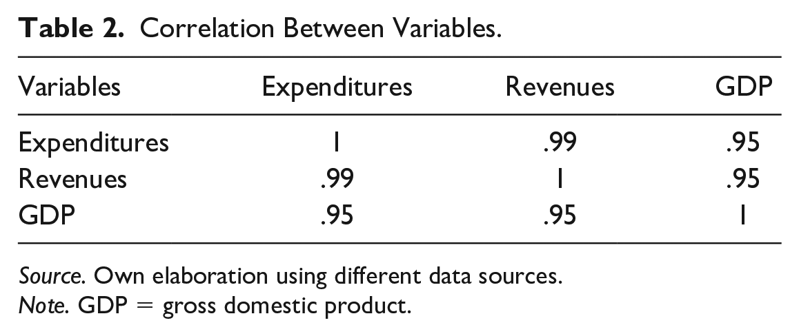
Source. Own elaboration using different data sources.

Note. GDP = gross domestic product.

Figure 2.

(A) Expenditure; (B) revenue; (C) GDP; (D) PE, PR, and GDP for Spain over the period 1880–2016; and (E) PE and PR as a percentage of GDP.

Table 2 displays the high correlation between the variables with a value of .99 between revenues and expenditures and .95 between GDP and expenditures or revenues.

The figures show the individual and joint evolution of the variables.

The individual figures (Figure 2A–2C) represent the evolution of expenditure, revenue, and GDP in the period 1880–2016.

Figure 2D provides PE, PR, and GDP for Spain over the period 1880–2016, whereas Figure 2E represents PE and PR as a percentage of GDP. The PE and PR data until 2011 are taken from Mauro et al. (2013), whereas data from later years are taken from Eurostat (2016b). As for GDP, data are taken from Barro and Ursua (2008) until 2008 and from Eurostat (2016a) for 2016. The values in Figure 2D are in millions of real Euros, adjusted for inflation to the corresponding 2006 value.

Until 1920, PE, PR and GDP remained relatively stable and slowly increased thereafter. In 1940, PE slightly increased with respect to 1935, but oscillated up and down in the following years, coinciding with the events of World War II. Spain remained neutral in this conflict, although it sent troops (the Blue Division) to fight alongside the Nazis. When the conflict ended, it resulted in a significant drop in PE due to a decrease in defense spending; the spending levels of 1935 were not reached again until 1958. PR developed similarly. After World War II, in 1946, PR decreased and the 1935 values were reached 12 years later, in 1958. GDP reached a maximum in 1935, a value which was not reached again until 1952. In per capita terms, PE developed in the same manner; the value increased in 1940 with respect to 1935 and was maintained after the Spanish Civil War and throughout World War II. However, once this period had ended, it dropped below 1935 values and did not recover until 1962.

In later periods, there was a possible structural breakpoint with the advent of democracy (1976). In 1976, the PR/GDP ratio was 11.92%, whereas in 1983, it was 21.18%. However, this value did not proceed to drop; the ratio was either maintained or grew slowly in the subsequent years. PE/GDP developed similarly, moving from 11.48% to 25.86% (indeed, for the first time in history, Spain had been showing fiscal deficits). However, as opposed to what was proposed by PW, none of the variables studied decreased in later years, although values stabilized at the end of the 1980s. Whether or not this period constituted a displacement effect consistent with PW will later be tested.

PR/GDP increased again in the middle of the 1990s. After Expo ’92 in Seville and the 1992 Summer Olympics in Barcelona, there was stagnation in the Spanish economy, given a corresponding drop in public and private construction. During this period of contraction, PE decreased, whereas both PR and PR/GDP increased.

Finally, the most recent period of contraction in Spain, corresponding to the Great Recession of 2008, resulted in significant repercussions in 2010, with a strong drop in all three variables. However, both PE/GDP and PR/GDP remained constant.

Upon interpreting the displacement effect, we considered tolerable tax burden from the perspective of both direct and indirect tax increases, in absolute and relative terms. Tax increases allow governments to increase PE; for PW, this corresponds specifically to war expenditures. This increase in taxes does not subsequently revert to its initial level, but instead is maintained, meaning that while PE can decrease slightly, it never returns to its initial values. This interpretation of the displacement effect is associated with the relationship between PR and PE, known in the literature as the Revenues–Expenditures Nexus; however, this connection only applies in periods of structural break. We propose testing the displacement effect, considering the relationship between PR and PE and using GDP as a control variable. In addition, dummy variables must be introduced for the period of structural break.

The following equations are presented:

$$\begin{array}{l}{\mathrm{LnPE}}_{{\mathrm{cap}}_t}={\alpha }_0+{\alpha }_1{\mathrm{LnPR}}_t+{\alpha }_2{\mathrm{LnGDP}}_t\\ +{\beta }_1{D}_1+{\beta }_2{D}_2+{\beta }_3{D}_3+{\beta }_4{D}_4+{\epsilon }_t,\end{array}$$

(1)

$$\begin{array}{l}\frac{\mathrm{LnPE}}{{\mathrm{GDP}}_t}={\alpha }_0+{\alpha }_1\frac{\mathrm{LnPR}}{{\mathrm{GDP}}_t}+{\alpha }_2{\mathrm{LnGDP}}_{{\mathrm{cap}}_t}\\ +{\beta }_1{D}_1+{\beta }_2{D}_2+{\beta }_3{D}_3+{\beta }_4{D}_4+{\epsilon }_t,\end{array}$$

(2)

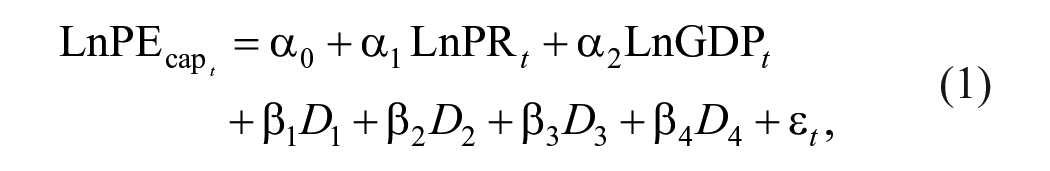
where dummy variables D_i refer to the breakpoints obtained, taking a value of 0 for periods before the breakpoint and 1 for periods afterward. If any of the coefficients are significant, it could indicate the existence of a possible displacement in PE in line with PW.

Figure 3 presents the variables to be used in the empirical analysis.

Figure 3.

(A) PE/GDP; (B) PE_cap; (C) PR/GDP; and (D) GDP_cap.

Given the nature of the series, we must consider its possible nonstationarity. To do so, unit root tests were conducted, specifically augmented Dickey–Fuller (ADF), Phillips–Perron (PP), and Kwiatkowski, Phillips, Schmidt, and Shin (KPSS) tests. In the first two, the null hypothesis is the existence of a unit root, whereas in the last, it corresponds to the stationarity of the series.

Table 3 shows that the series are I(1) but not I(2).

Table 3.

Series Unit Root Tests.

Variables	ADF (5% critical value)	PP (5% critical value)	KPSS (5% critical value)
LnPEcap	1.06 (−2.88)	0.56 (−2.88)	1.28 (0.46)
LnPR	1.27 (−2.88)	0.73 (−2.88)	1.29 (0.46)
LnGDP	0.65 (−2.88)	0.70 (−2.88)	1.34 (0.46)
LnPE/GDP	−1.95 (−3.44)	−2.48 (−3.44)	0.21 (0.14)
LnPR/GDP	−1.71 (−3.44)	−2.55 (−3.44)	0.24 (0.14)
LnGDPcap	−2.74 (−3.44)	−2.50 (−3.44)	0.28 (0.14)
∆LnPEcap	−7.34 (−1.94)	−15.57 (−1.94)	0.25 (0.46)
∆LnPR	−19.46 (−1.94)	−17.91 (−1.94)	0.31 (0.46)
∆LnGDP	−8.55 (−1.94)	−8.55 (−1.94)	0.32 (0.46)
∆LnPE/GDP	−18.64 (−1.94)	−17.58 (−1.94)	0.13 (0.46)
∆LnPR/GDP	−5.73 (−1.94)	−9.16 (−1.94)	0.36 (0.46)
∆LnGDPcap	−21.52 (−1.94)	−21.13 (−1.94)	0.16 (0.46)

Source. Own elaboration using different data sources.

Note. In parentheses, 5% critical value is given. ADF = augmented Dickey–Fuller; PP = Phillips–Perron; KPSS = Kwiatkowski, Phillips, Schmidt, and Shin.

Given that all the series demonstrate structural breaks, it is appropriate to test for unit roots with respect to the corresponding points. We have employed the standard tests for structural breakpoints, namely, those of Perron (P), Zivot–Andrews (ZA), Lumsdaine–Papell (LP), and ADF. The first two and the fourth tests detect a breakpoint endogenously, whereas the third detects two breakpoints.

Table 4 presents the obtained results.

Table 4.

Series Unit Root Tests With Structural Breaks.

Variables	P (5% critical value) (Date of structural breakpoint)	ZA (5% critical value) (Date of structural breakpoint)	LP (5% critical value) (Date of structural breakpoint)	ADF Unit roots with structural breaks
LnPEcap	−4.40 (−5.23) (1960)	−4.41 (−4.93) (1961)	−6.04 (−6.16) (1935,1960)	−4.13 (−4.44) (1977)
LnPR	−2.80 (−5.23) (1979)	−2.89 (−4.93) (1980)	−4.61 (−6.16) (1960,1982)	−2.68 (−4.44) (1957)
LnGDP	−4.32 (−5.23) (1960)	−4.34 (−4.93) (1961)	−5.88 (−6.16) (1929,1960)	−3.56 (−4.44) (1950)
LnPE/GDP	−5.15 (−5.23) (1982)	−5.17 (−4.93) (1983)	−6.83 (−6.16) (1945,1980)	−5.15 (−4.44) (1982)
LnPR/GD	−5.15 (−5.23) (1982)	−5.17 (−4.93) (1983)	−7.13 (−6.16) (1945,1982)	−4.35 (−4.44) (1980)
LnGDPcap	−4.33 (−5.23) (1960)	−4.34 (−4.93) (1961)	−5.81 (−6.16) (1929,1960)	−3.57 (−4.44) (1950)
∆LnPEcap	−11.21 (−5.23)	−9.71 (−4.93)	−6.77 (−6.16)	−11.23 (−4.44)
∆LnPR	−9.35 (−5.23)	−8.26 (−4.93)	−6.86 (−6.16)	−20.81 (−4.44)
∆LnGDP	−10.96 (−5.23)	−9.51 (−4.93)	−6.64 (−6.16)	−11.00 (−4.44)
∆LnPE/GDP	−7.82 (−5.23)	−5.17 (−4.93)	−6.84 (−6.16)	−5.35 (−4.44)
∆LnPR/GDP	−10.15 (−5.23)	−8.09 (−4.93)	−7.07 (−6.16)	−22.59 (−4.44)
∆LnGDPcap	−10.93 (−5.23)	−9.49 (−4.93)	−6.64 (−6.16)	−10.88 (−4.44)

Source. Own elaboration using different data sources.

Note. In parentheses, 5% critical value and date of structural breakpoint are given. P = Perron; ZA = Zivot–Andrews; LP = Lumsdaine–Papell; ADF = augmented Dickey–Fuller.

Table 4 shows that the series are I(1) and the breakpoints for each series.

However, as we are interested in the set of breakpoints in the two equations, we have performed a Bai–Perron test. The results are displayed in Table 5.

Table 5.

Bai–Perron Breakpoint Test.

Equations	Breakpoint test	F-statistic	Scaled F-statistic	Critical value
Equation 1	0 vs. 1*	531.67	1,595.03	13.98
	1 vs. 2*	75.90	227.70	15.72
	2 vs. 3*	89.66	268.98	16.83
	3 vs. 4*	7.14	21.43	17.61
	4 vs. 5	1.10	3.31	18.14
			Sequence	Partition
		1	1963	1911
		2	1988	1944
		3	1921	1963
		4	1944	1988
Equation 2	0 vs. 1*	15.45584
	1 vs. 2*	14.47058
	2 vs. 3*	10.08536
	3 vs. 4*	11.27182
	4 vs. 5	3.413178
			Sequence	Partition
		1	1978	1912
		2	1909	1952
		3	1997	1978
		4	1952	1997

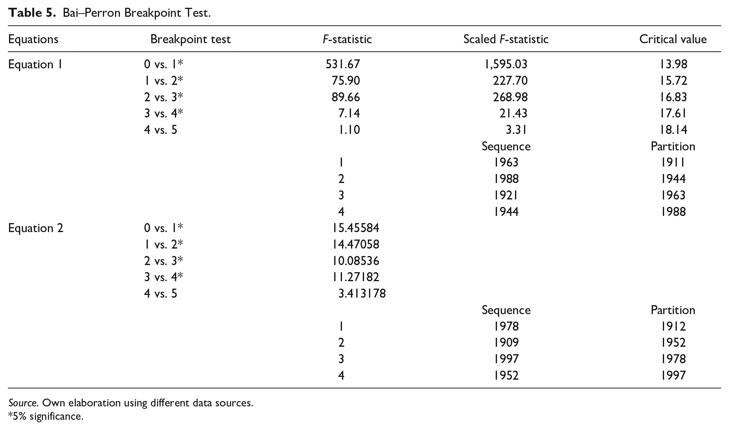
Source. Own elaboration using different data sources.

*

5% significance.

The Bai–Perron test is sequential; it tests the existence of L + 1 breakpoints against L breakpoints. Neither the number of breakpoints nor their times are known beforehand. Breakpoints were observed in 1911, 1944, 1963, and 1988 for the first equation, whereas they were observed in 1912, 1952, 1978, and 1997 for the second. The breakpoints in the first equation correspond to the two world wars, the beginning of the opening of the Spanish economy and the beginning of the period of economic expansion in Spain. Those of the second equation correspond more so with the periods observed in the figures. The year 1912 corresponds to World War I, 1952 corresponds to a recovery of 1935 values, 1978 corresponds to the beginning of democracy, and 1997 coincides with preparation to enter the Economic and Monetary Union of the European Union.

Given this instability and the presence of structural breakpoints in the equations, it is appropriate to analyze possible cointegration in each of the equations, performing tests that take into account these structural breakpoints.

Initially, different tests were considered without taking the structural breakpoints into account. These included tests for only one equation, specifically the Engle–Granger (EG) and Phillips–Ouliaris (PO) tests, as well as a multi-equation test, namely, the Johansen–Juselius (JJ) test. Tables 6 and 7 present the results for both sets.

Table 6.

EG and PO Tests.

	EG test		PO test
Models	τ-statistics	p	τ-statistics	p
Model 1	−4.62	.00	4.57	.00
Model 2	−4.62	.00	−4.58	.00

Source. Own elaboration using different data sources.

Note. EG = Engle–Granger; PO = Phillips–Ouliaris.

Table 7.

JJ Cointegration Test.

Models	Null hypothesis	Eigenvalue	Trace statistic	Critical value 0.05	Maximum eigenvalue statistic	Critical value 0.05
Model 1	r = 0	0.14	35.81	35.19	29.90	22.29
	r ≤ 1	0.08	15.90	20.26	11.63	15.89
	r ≤ 2	0.03	4.27	9.16	4.27	9.16
Model 2	r = 0	0.15	35.91	29.79	21.84	21.13
	r ≤ 1	0.10	14.07	15.49	14.06	14.26
	r ≤ 2	5.16E−0.5	0.006	3.84	5.16E−0.5	3.84

Source. Own elaboration using different data sources.

Note. JJ = Johansen–Juselius.

The EG and PO tests reject the null hypothesis of no cointegration for both equations, whereas the JJ test rejects r = 0 and accepts r ≤ 1 in both equations. As such, cointegration is confirmed in both equations, without considering breakpoints.

Considering breakpoints, we performed Gregory–Hansen (GH) tests for one equation, which endogenously detected a breakpoint. We also performed a Johansen–Mosconi–Nielsen (JMN) test, in which one or two breakpoints can be considered in the variables by level (In JMN1, none of the time series show a trend, but the cointegration relationships exhibit a drift that may differ between subsamples (corresponds to H_c(r) in JMN, 2000). In JMN2, some or all of the series show a trend in each subsample, and the cointegration ratios show a stationary trend in all subsamples; breaks in the trend in the cointegration ratios and in nonstationary series are allowed (corresponds to H_l(r) in JMN, 2000) (Table 8).

Table 8.

Cointegration Tests With Structural Breakpoints.

Cointegration tests	Model 1	Breakpoint	Model 2	Breakpoint
GH (critical value)	−3.06 (−4.92)	1914	−3.94 (−4.92)	1990
JMN1	77.15 (76.97)46.14 (54.08)	1911,1944	35.49 (34.80)15.05 (28.58)	1912,1952
JMN2	93.63 (88.80)53.44 (63.78)	1911,1944	69.10 (88.80)40.41 (63.87)	1912,1952
JMN1	84.55 (76.97)50.14 (54.07)	1963,1988	83.02 (76.92)52.90 (54.07)	1978,1997
JMN2	71.71 (69.81)41.35 (47.85)	1963,1988	70.43 (69.82)43.99 (47.85)	1978,1997

Source. Own elaboration using different data sources.

Note. GH = Gregory–Hansen.

The GH test holds the absence of cointegration as a null hypothesis and uses the ADF as a test statistic. In our case, we determine that the series are not cointegrated. However, the JMN tests indicate cointegration (r ≤ 1) in the first equation for 1911 and 1944 as breakpoint dates, as well as for 1963 and 1988. The second equation shows cointegration (r ≤ 1) for 1912 and 1952, whereas JMN1 shows cointegration for 1978 and 1997 even while JMN2 does not.

The cointegration equations are obtained based on the previous results. In this case, FMOLS were used. For the first equation, the following dummy variables were utilized: D₁ for 1911, D₂ for 1944, D₃ for 1963, and D₄ for 1988. Each variable took a value of 0 before the considered date and a value of 1 after that date. These dummy variables as used with the variables LnPR and LnGDP. The significant values of the first dummy variables indicate drift of the origin ordinate, whereas those of the second indicate changes in the slope or, equivalently, in the elasticity of PE with respect to PR or PE (Table 9).

Table 9.

Cointegration Equations for Model 1.

Variable	Equation 1	Equation 2	Equation 3
	Coefficient (t-statistic)	Coefficient (t-statistic)	Coefficient (t-statistic)
LnPR	1.29 (15.88)	1.35 (13.14)	1.43 (17.53)
LnGDP	−1.37 (−13.29)	−0.46 (−4.25)	−0.52 (−5.24)
C	6.17 (10.39)	2.17 (3.69)	2.04 (4.31)
D 1	0.02 (0.62)
D 2	−0.10 (−1.31)
D 3	−0.18 (−3.04)		−3.48 (−0.46)
D 4	0.16 (2.39)		0.10 (1.59)
D1PR		0.19 (1.29)
D2PR		−0.66 (−3.73)	−0.32 (−2.21)
D3PR		−1.73 (−1.89)	−1.86 (−2.32)
D4PR		0.67 (1.35)
D1GDP		−0.15 (−1.29)
D2GDP		0.57 (3.72)	0.28 (2.14)
D3GDP		1.61 (1.83)	1.98 (1.97)
D4GDP		−0.61 (−0.36)
R 2	.97	.99	.996

Source. Own elaboration using different data sources.

For the second equation, the following dummy variables were used: D₁ for 1912, D₂ for 1952, D₃ for 1978, and D₄ for 1997. These dummy variables were combined with the variables LnPR/GDP and LnGDP_cap. The significance is the same as in the preceding paragraph (Table 10).

Table 10.

Cointegration Equations for Model 2.

Variable	Equation 1	Equation 2	Equation 3
	Coefficient (t-statistic)	Coefficient (t-statistic)	Coefficient (t-statistic)
LnPR/GDP	1.30 (15.89)	1.37 (13.82)	1.43 (17.53)
LnGDPcap	−0.07 (−1.65)	−0.12 (−2.28)	−0.08 (−2.89)
C	5.89 (13.42)	6.45 (14.19)	6.32 (17.07)
D 1	0.02 (0.62)
D 2	−0.10 (−1.31)
D 3	−0.18 (−3.04)		−3.12 (−0.57)
D 4	0.16 (2.39)		0.10 (1.60)
D1*LnPR/GDP		0.20 (1.45)
D2*LnPR/GDP		−0.67 (−3.89)	−0.31 (−2.19)
D3*LnPR/GDP		−1.70 (−1.82)	−1.87 (−2.33)
D4*LnPR/GDP		0.54 (0.29)
D1*LnGDPcap		0.05 (1.40)
D2*LnGDPcap		−0.12 (−3.81)	−0.06 (−2.66)
D3*LnGDPcap		−0.16 (−1.82)	0.12 (1.60)
D4*LnGDPcap		0.06 (0.35)
R 2	.97	.98	.98

Source. Own elaboration using different data sources.

We obtain the following results.

We analyzed the results for Model 1 that were obtained in the third equation, which summarizes the two previous equations given it only retains the significant variables. A measurable displacement effect was observed at breakpoints corresponding to 1963 and 1988. However, in this equation, the dummy variables corresponding to a displacement in the drift are not significant; as such, we have limited ourselves to those corresponding to the combined variables. For D₂, revenue elasticity decreases from 1.43 to 1.11, whereas GDP elasticity increases from −0.52 to −0.24. In other words, in a period of crisis, an increase in PR corresponds to an increase in PE, but to a lesser extent than what would have existed without a crisis. The opposite occurs with respect to GDP; if this value decreases, PE increases, such that PE exhibits countercyclical behavior. The same reasoning can be applied with respect to the second breakpoint, corresponding to 1988. Revenue elasticity is −0.43, which indicates that PR is developing over this period in a manner contrary to that of PE. Meanwhile, GDP elasticity is positive, at 1.46, meaning that PE is changing in the same direction as GDP for this period. As such, we can affirm that the displacement effect explains the development of PE in Spain in the crises in 1963 and 1988, even while it is not a valid explanation for the other two.

Model 2 also takes Equation 3 into account. The coefficients of the independent variables are significant in the three equations. Revenue elasticity is greater than 1, whereas GDP elasticity is negative. The dummy variables that affect the constant are not significant, such that there is no displacement in the drift. With respect to revenue, the dummy variables correspond to Periods 2 and 3, both recessive, are negative, which indicates a decrease in revenue elasticity in both periods. This negative elasticity could transform in the third period, which would indicate that PE develops in a manner contrary to PR. When considering GDP_cap, only the coefficient corresponding to the second period is significant, although it is minimal, which indicates that no variation is produced in the elasticity of PE with respect to GDP_cap. A degree of displacement can only be observed close to the year 1978, in which the ratio increased notably and did not return to the initial value in subsequent years.

To test the ratchet effect, we based our approach on that of Hercowitz and Strawczynski (2004), Durevall and Henrekson (2011), and Grenade and Wright (2014). The following equation was formulated:

$$\begin{array}{c}\frac{\Delta \mathrm{LnPE}}{{\mathrm{GDP}}_t}={\alpha }_0+{\alpha }_1\frac{\Delta \mathrm{LnPE}}{{\mathrm{GDP}}_{t-1}}+{\alpha }_2\frac{\Delta \mathrm{LnPE}}{{\mathrm{GDP}}_{t-2}}\\ +{\beta }_{1p}{\left({\mathrm{LnGDP}}_{\mathrm{cap}}-\tau \right)}_t^p+{\beta }_{2p}{\left({\mathrm{LnGDP}}_{\mathrm{cap}}-\tau \right)}_{t-1}^p\\ +{\beta }_{1N}{\left({\mathrm{LnGDP}}_{\mathrm{cap}}-\tau \right)}_t^N\\ +{\beta }_{2N}{\left({\mathrm{LnGDP}}_{\mathrm{cap}}-\tau \right)}_{t-1}^N+{\epsilon }_t.\end{array}$$

(3)

From the above equation, the long-term solution was calculated, obtaining

$$\begin{array}{l}\frac{\Delta \mathrm{LnPE}}{{\mathrm{GDP}}_t}=\alpha +{\beta }_p{\left({\mathrm{LnGDP}}_{\mathrm{cap}}-\tau \right)}^P\\ +{\beta }_N{\left({\mathrm{LnGDP}}_{\mathrm{cap}}-\tau \right)}^N,\end{array}$$

(4)

where ${\beta }_P=[({\beta }_{1p}+{\beta }_{2P})/(1-{\alpha }_1+{\alpha }_2)]$ and likewise for β _N , τ is the trend of GDP_cap or business cycle; P and N represent positive and negative deviations from the trend, corresponding to expansive and recessive periods, respectively. The hypothesis states that, given ${\mathrm{Ln(PE/GDP)}}_{t-1}$ , PE/GDP grows over time because recessions increase Ln(PE/GDP) more than expansions reduce it, due to asymmetry. For the hypothesis to hold, the long-term coefficient that corresponds to expansive periods must be greater than its recessive counterpart, as long as the fiscal policy undertaken is procyclical (that is to say, β _p > β _N ). When the policies are countercyclical, the relationship will hold between the absolute values of both variables, and in that case, the long-term coefficient of the recessive periods will be greater than its expansive counterpart during expansive periods|β _N | >|β _P | This analysis considers the complete sample and the subsample corresponding to the period after the Spanish Civil War. The following results are obtained (Table 11).

Table 11.

Equations for the Ratchet Effect.

Coefficients	Complete sample (1880–2016)		Sample after the Spanish Civil War (1940–2016)
${\alpha }_0$	0.002 (0.11)
${\alpha }_1$	−0.35 (−3.97)	−0.43 (−5.57)	−0.33 (−2.88)	−0.32 (−2.93)
${\alpha }_2$	0.12 (1.44)		−0.008 (−0.28)
${\beta }_{1p}$	0.24 (0.38)	−0.02 (−0.04)	0.38 (0.37)	0.17 (0.19)
${\beta }_{2p}$	0.01 (0.02)	0.34 (0.51)	0.58 (0.56)	0.51 (0.56)
${\beta }_{1N}$	−1.68 (−2.19)	−1.76 (−2.41)	−2.47 (−2.08)	−2.30 (−2.16)
${\beta }_{2N}$	1.10 (1.39)	0.99 (1.35)	1.60 (1.30)	1.69 (1.61)
${\beta }_p$	0.21		0.72
${\beta }_N$	−0.47		−0.64
R 2	.24		.15
χ2	0.95 (0.32)		1.40 (0.23)

Source. Own elaboration using different data sources.

Only the coefficient corresponding to the recessive portion is significant; the fiscal policy is countercyclical. In other words, in a recessive period, PE/GDP increases, which can be attributed to an increase in PE, a decrease in GDP, or to both simultaneously. The coefficient for the initial and delayed variable was not significant in the expansive part but it is positive, which would indicate that the fiscal policy is procyclical. In other words, increases in GDP provoke an increase in PE. As for the long-term coefficients, the sign is the same as for the short-term coefficients, whereas chi-square indicates that said coefficients cannot be differentiated. As such, the ratchet effect is not supported.

An Alternative Explanation of the Displacement Effect Using Wavelet Methodology

Wavelet analysis has emerged as an alternative to Fourier analysis (Aguiar-Conraira & Soares, 2014).

Using Fourier analysis, it is possible to study time series in the frequency domain. However, using a Fourier transform, the temporal information is lost, making it difficult to distinguish transient relations or to identify structural changes. Therefore, the technique is only appropriate for stationary time series. On the contrary, wavelet analysis estimates the spectral characteristics of a time series as a function of time, revealing how its different periodic components change over time. In addition, wavelet analysis allows for the identification of possible breakpoints in each period of time and frequency.

Wavelet methodology is based on a “mother” function, ψ; the square of this function is integrable and it fulfills a technical condition known as admissibility. In most applications, the wavelet function must be well localized, both in the time and frequency domains. In such a case, the admissibility condition is reduced to requiring ψ to have a mean of zero, in other terms, ${\int }_{-\infty }^{\infty }\psi (t)dt=0$ . This means that the ψ function has an upward and downward ripple along the t-axis, meaning that it behaves like a wave; this, together with the property of gradual drop-off, justifies the choice of the term wavelet for ψ.

Beginning with a mother wavelet ψ, a family ψ_τ,s of “wavelet children” can be obtained by taking a scaling factor and translating ψ:

$${\psi }_{\tau ,s}=\frac{1}{\sqrt{s}}\psi \left(\frac{t-\tau }{s}\right),$$

(5)

where s, τ Є R and s ≠ 0, in which s is a scaling or dilation factor that controls the wave width (the factor $1/\sqrt{s}$ is introduced to guarantee that energy ║ψ_τ,s║ = 1) and τ is the translation parameter that controls the location of the wavelet in time. Increasing s decreases the frequency of the wavelet, allowing it to measure long-term cycles, whereas decreasing it increases the frequency, allowing for the measurement of short-term cycles. Meanwhile, translation simply refers to changing the position in time.

The continuous wavelet transform of a given time series x(t), with respect to the wavelet ψ, is a function of two variables, W_x(τ,s):

$$W_{x;\psi }\left(\tau ,s\right)=\underset{-\infty }{\overset{\infty }{\int }}x\left(t\right)\frac{1}{\sqrt{\left|s\right|}}\overline{\psi }\left(\frac{t-\tau }{s}\right)dt\mathrm{,}$$

(6)

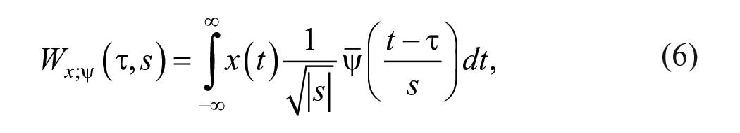
where the top bar denotes the complex conjugate. The transform is considered complex because ψ is assumed to be complex. The wavelet transform projects the variable in the time–scale domain. It is said that wavelet analysis is performed in the time–frequency domain because there is a one-to-one relationship between scales and frequencies and both terms can be used interchangeably.

As with the terminology used in the case of Fourier transform, the wavelet power spectrum, sometimes called the wavelet scalogram or periodogram, is defined as follows:

$${\left(\mathrm{WPS}\right)}_x\left(\tau ,s\right)={\left|W_x\left(\tau ,s\right)\right|}^2.$$

(7)

This provides a measure of the distribution of variance of the time series in the time–frequency plane. As opposed to the classical power spectrum based on Fourier transform, (WPS) _x (τ,s) indicates how the concentration of time series x(t) is distributed in both the frequency and time domains.

If quantitative information is needed on the phase interactions between two time series, it is best to choose continuous and complex wavelets. When we choose a complex wavelet, the wavelet transform is also complex. In this case, the transform can be separated into its real part $\Re$ (W_x) and its imaginary part $\Im$ (W_x) or its amplitude $\left|W_x\mathrm{(}\tau ,s)\right|\mathrm{and}\mathrm{phase}\Phi x\mathrm{(}\tau ,s\mathrm{)}$ , whereby

$$W_x\left(\tau ,s\right)=\left|W_x\left(\tau ,s\right)\right|e^i{\Phi }_x^{\left(\tau ,s\right)}.$$

(8)

The phase angle $\Phi x\mathrm{(}\tau ,s\mathrm{)}$ of the complex number W_x $\mathrm{(}\tau ,s)$ can be obtained from the formula

$$\Phi \left(\tau ,s\right)=\mathrm{Arctan}{\left(\frac{\Im \left\{W_x\left(\tau ,s\right)\right\}}{\Re \left\{W_x\left(\tau ,s\right)\right\}}\right)}^2,$$

(9)

using the signs of the denominator and numerator to determine the quadrant in which the angle belongs. For functions with real values, the imaginary part is 0 and the phase is not defined. Therefore, to separate the phase and amplitude information from a time series, it is necessary to use complex wavelets. In these cases, it is convenient to choose ψ(t) so that it is progressive or analytic—in other words, so that $\widehat{\psi }=0$ for f < 0. In fact, when $\psi$ is analytic and x(t) is real, it is possible to reconstruct x(t) considering only positive values of the scaling parameter s. Analytic wavelets are ideal for the analysis of oscillatory signals given that the analytic wavelet transform continues to provide an estimate of the instantaneous amplitude and of the instantaneous signals in the vicinity of each time–scale localization $\mathrm{(}\tau ,s)$ .

There are various kinds of available wavelet functions with different characteristics, such as Morlet, Mexican hat, Haar and Daubichies. Given that the coefficients of W_x $\mathrm{(}\tau ,s)$ contain a combination of information on $x\psi \mathrm{(}t\mathrm{)}$ , selecting the appropriate wavelet is crucial—the purpose of its application must be taken into consideration.

For economic applications, the Morlet wavelet is normally used; it has an optimal time–frequency concentration.

The concepts of cross-wavelet transform, wavelet coherence (WC), and phase difference are natural generalizations of wavelet analysis instruments that permit us to work with time–frequency dependencies between two time series.

The cross-wavelet transform of two series x(t) and y(t) is defined as follows:

$$W_{xy}\left(\tau ,s\right)=W_x\left(\tau ,s\right)\overline{W_y\left(\tau ,s\right),}$$

(10)

where W_x and W_y are the wavelet transforms of x and y, respectively. Cross-wavelet power is defined as $\left|W_{xy}(\tau ,s)\right|$ . The cross-wavelet power describes the local covariance between two series for every value of time and frequency. Therefore, the cross-wavelet power gives us a quantified indication of the similarity of power between the two time series.

Analogous to the concept of coherence used in Fourier analysis, given two time series x(t) and y(t), their WC is defined as follows:

$$R_{xy}\left(\tau ,s\right)=\frac{\left|S\left(W_{xy}\left(\tau ,s\right)\right)\right|}{\sqrt{S\left(\left|W_{xx}\left(\tau ,s\right)\right|\right)S\left(\left|W_{yy}\left(\tau ,s\right)\right|\right)}},$$

(11)

where S denotes a smoothing operator in time and frequency. It ranges from 0 (no coherence) to 1 (strong coherence). This quantity can be interpreted as the coefficient of local correlation in the time–frequency space. When compared with cross-wavelet power, WC has the advantage of being normalized by the power spectrum of the two time series.

As has been seen previously, one of the main advantages of using a complex wavelet is that we can calculate the phase of the wavelet transform of each series, thereby obtaining information relating to the possible oscillation lag of the two series as a function of time and scale/frequency, ultimately yielding the phase difference. The phase difference can be calculated via the cross-wavelet transform using the following formula:

$${\phi }_{xy}\left(\tau ,s\right)=\mathrm{Arctan}\left(\frac{\Im \left\{S\left(W_{xy}\left(\tau ,s\right)\right)\right\}}{\Re \left\{S\left(W_{xy}\left(\tau ,s\right)\right)\right\}}\right).$$

(12)

The sign information of each part completely determines the value of φ _xy Є (−п, п). A phase difference of 0 indicated that the series move together at the specified frequency; if φ _xy Є (0, п/2), the series move in phase, but series x leads series y; if φ _xy Є (−п/2, 0), y leads x. A phase difference of п (0, −п) indicates an antiphase relationship; if φ _xy Є (п/2, п), y leads x, whereas x leads y if φ _xy Є (−п, −п/2).

With the phase difference, it is possible to calculate the instant delay time between the two time series $\Delta T={\phi }_{xy}/\omega (s)$ .

Wavelet analysis was performed for the relationship between LnPE/GDP and LnGDP. Two analysis instruments were used: WC and the phase difference and time delay between the variables.

WC can be considered a correlation coefficient over time and frequency. Therefore, it can be used to detect common oscillations localized in time in nonstationary signals (time series). In situations where it is natural to see that a time series is influencing another, we can use the cross-spectrum phases to identify the relative delay between the two series.

Figures are provided containing both the Wavelet Power Spectrum (WPS) of LnPE/GDP and the WC between LnPE/GDP and LnGDP. These make it possible to determine whether Wagner’s law or the displacement effect allows us to explain PE growth over the long term. If Wagner’s law is relevant for the growth in PE/GDP, then significant regions of wavelet coherence with GDP leading will coincide with those of the WPS in time–frequency space. Alternatively, if the displacement effect plays a significant role in explaining the growth, these agreements will not be observed and the long-term rise in crisis periods must show an upward change in WPS at lower frequencies.

Figure 4 plots the number of years considered (1880–2016) along the x-axis, whereas the y-axis contains the frequencies or periods of time in years. It displays the WPS of LnPE/GDP. WPS indicates how the concentration of the time series is distributed in the frequency domain and in the time domain. The black lines indicate the cone of influence; the results are not reliable outside of these lines. Meanwhile, Figure 5 shows the WC.

Figure 4.

WPS of LnPE/GDP.

Figure 5.

Wavelet coherency LnPE/GDP LnGDPcap.

In the WPS, a highly significant region of power was observed in the period between 1920 and 2000 at low frequencies between 16 and 32 years.

Figure 6 shows phase differences. Phase differences corresponding to periodicity cycles between 1 and 4, 4 and 8, 8 and 16, and 16 and 32 years in length were considered.

Figure 6.

Phase differences.

As has been analyzed previously, the phase difference can have a range of φ _xy Є (−п, п). A phase difference of 0, φ _xy = 0, indicates that the series move together at the specified frequency, meaning they are completely and positively correlated; if φ _xy Є (0, п/2), the series move in phase, but series x leads series y; if φ _xy Є (−п/2, 0), y leads x. A phase difference of п (0–п) indicates an antiphase relationship; if φ _xy Є (п/2, п), y leads x, whereas x leads y if φ _xy Є (−п, −п/2).

The phase difference figures show, in general, that LnPE/GDP leads LnGDP. The inverse is only true in the initial period, with a structural breakpoint around 1900 and a second between 1940 and 1970 for the 4- to 8-year frequency band. However, the 16- to 32-year frequency band shows LnGDP leading LnPE/GDP between roughly 1985 and 2016. Thus, in none of the frequency bands does LnGDP lead LnPE/GDP, meaning that Wagner’s law is rejected for the considered period of 1880–2016.

On the contrary, a region of strong coherence is observed on the WPS between approximately 1920 and 1980 at low frequencies for periods between 16 and 32 years. This does not coincide with the significant region in WC that extends from 1900 to 1920 and then from 1980 to 2000. Therefore, we can affirm that the displacement effect can explain a large part of the growth in Spanish PE over the considered period.

Conclusion

In the previous sections, we have studied two alternative explanations of Wagner’s law of growth in PE. The displacement hypothesis was formulated as a response to the inability of Wagner’s law to explain the long-term evolution of PE in Great Britain. Meanwhile, the ratchet effect seeks to explain theoretical and empirical inconsistencies in the displacement effect. These explanations have not received the same empirical attention as Wagner’s law; more specifically, in the case of Spain, the former has only been tested by Comín (1985) and Jaén-García (1998), whereas the latter has not been addressed at all. Recently, Funashima (2017) has studied the displacement effect, whereas Durevall and Henrekson (2011) have studied both the displacement effect and the ratchet effect.

This article has reviewed the different empirical approaches in the literature review and attempted to provide original contributions. Both effects were tested, considering PR as an independent variable. In addition, the displacement effect was tested using wavelet analysis, which allowed for the results to be compared with those obtained using the other methodology.

The displacement effect explains the development of PE in Spain in the crises of 1963 and 1988. Wavelet analysis affirmed that a displacement effect was produced in the crises between 1920 and 1980, fundamentally the crises after the Spanish Civil War and the opening of the Franco’s regime at the end of the 1960s, ultimately leading to the conversion of the Spanish dictatorship to a democratic regime.

Meanwhile, no support was observed for the ratchet effect.

In summary, the data and equations that were employed indicate that the development of PE in Spain can be partially explained using the displacement effect, but not with the ratchet effect.

The events that have occurred in the Spanish economy make it possible to understand how the displacement effect helps to explain the evolution of public expenditure in Spain. Initially, we consider the structural breakpoints detected by the analysis using unit roots and cointegration.

Considering the order presented, the break in 1963 would be explained by the decline of Franco’s dictatorship. The years between 1960 and 1975 witnessed the last period of said dictatorship. In 1959, the Stability Plan began, which eventually drove economic growth–GDP increased, in real terms, at an annual rate above 7% over the course of the following 15 years. This growth was made possible, thanks to the return of Spain to the international economic scene, after 20 years of autocratic isolation, which allowed the country to take advantage of the expansion of developed countries, which were also experiencing unprecedented growth. However, public expenditure was very low. The Spanish economy had an extensive range of regulations, yet revenue service intervention was very limited. Public expenditure, in real terms, was lower than 25% GDP. During the first period, it remained below 20% GDP (19.5% in 1965), unlike the rest of the countries in the European Union 15 (33.1%) and the OECD (26.9%). However, spending rose slightly in the final period (24.1% in 1975), albeit, at that time this percentage was 40.9% in the Euro zone and 34.4% for the OECD. Despite this slow growth, there were notable changes in the composition of spending with respect to previous periods; what is more, the economy recovered its levels from before the Civil War. Spending decreased on general services, defense, and public debt, whereas greater attention was devoted to economic and social services.

The displacement that took place in 1988 is also explained by political and social events that transpired. In 1986, Spain entered the European Economic Community. Increased spending was the result of the policies instated by the new government controlled by the Spanish Socialist Worker Party (PSOE, in Spanish) to establish a welfare state in Spain. The universalization of public health care and the increase in the number of pensioners through noncontributive pensions, in addition to the amount received by beneficiaries, contributed to greater public expenditure. Similarly, education was made obligatory until 16 years of age and agreements were made with the private education system by which the latter would receive subventions from the state to guarantee that education would be free for those between the ages of 6 and 16.

The wavelet analysis identifies structural breaks in 1920 and 1980. In 1919, World War I came to an end. Until 1920, spending, revenue, and GDP had remained quite stable in the Spanish Economy, at values near 10% GDP. A period of slight growth ensued from that point forward. Between 1895 and 1902, spending grew with respect to the previous period and a decrease took place between 1902 and 1912. However, at the beginning of the World War I, public expenditure grew by over 10% GDP. Subsequently, an upward trend began, which would last until 1920, during which time Spain enjoyed exceptional circumstances that drove significant economic growth, which was eventually followed by a period of economic stagnation in 1921–1923.

The structural break in 1980 is explained by events that occurred years prior. Following the establishment of democracy in Spain in 1976, a rapid expansion of public expenditure ensued. Said spending increased from 23.19% GDP to 42.5%, in line with OECD countries, whose spending averaged 47% GDP. Between 1976 and 1982, intense growth in public expenditure took place, with an accumulative annual rate, in nominal terms, of 25.5.%, which can be attributed to three factors: the political transition, the manifestation of the most severe consequences of the economic crisis and the existence of weak governments formed by the Union of the Democratic Center (UCD, in Spanish) and the strong opposition of the Spanish Socialist Worker Party (PSOE).