Sage Journals: Discover world-class research

Abstract

Contextualizing research on entrepreneurial team decisions (ETDs) is closely related to elaborating the influence of several team members (TMs) on group decisions. Therefore, this study shows how the metricized limit conjoint analysis (MLCA) provides a method to more accurately determine TMs’ influences. For doing so, this study introduces a new approach as a suitable alternative to directly ask for TMs’ influences by utilizing a detailed step-by-step instruction for further research. Moreover, this study theoretically underlines the usability and preferableness of this new approach and validates it with a simulation of 45,000 assessments nested within 5,000 artificial respondents. The results indicate a diverse application potential for researching ETDs in several contexts. In addition, an illustrative example shows how this conjoint approach can be of value in subsequent research projects. Therefore, the MLCA is of increased interest for both researchers and practitioners when focusing on ETDs in several contexts.

Keywords

Entrepreneurial team decisions team members’ influences metricized limit conjoint analysis simulation tutorial

Introduction

“the ‘entrepreneur’ in entrepreneurship is more likely

to be plural, rather than singular” (Gartner, Shaver, Gatewood, & Katz, 1994, p. 6)

Research on entrepreneurial team decisions (ETDs) has manifold facets. In fact, research on entrepreneurial teams (ETs) has attracted increasing interest from both a scientific and a practical perspective (confer, for example, Cooney, 2005; Schjoedt, Monsen, Pearson, Barnett, & Chrisman, 2013). Interestingly, research on team composition and its consequences is exceptional. Talaulicar, Grundei, and von Werder (2005), as one of these rare examples, focus on two distinct models on how ETs are organized. Based on findings of an empirical study, they identify an urgent need to distinguish between a departmental model (i.e., a horizontal division of labor) and a CEO model (i.e., a hierarchical relationship among team members [TMs]). Although this study is of huge benefit in terms of decision comprehensiveness and decision speed in ETDs, it remains open how to adequately measure these two types of team composition. In fact, the authors used two single-item questions for elaborating the departmental model or the CEO model (Talaulicar et al., 2005). As with any self-reported direct evaluation, indirect measures lead to more sophisticated results (confer, for example, Louviere & Islam, 2008; Srinivasan, 1988). Using such a procedure enables the researcher to elaborate consequences of a “hidden” CEO model (i.e., an unequal power distribution between TMs).

In a similar vein, Kocher, Strauß, and Sutter (2006) distinguish between two different ways of decision-making: individual or in a team. Although they identify causes and consequences of self-selection, consequences of a “hidden” individual decision (i.e., a team decision that is objectively made by a single individual) remain open. Even more specific, de Mol, Khapova, and Elfring (2015) highlight that “the way in which ET members work together plays an important role in determining venture outcomes” (p. 232). In addition, researchers frequently highlight the importance of ET composition (Muñoz-Bullon, Sanchez-Bueno, & Vos-Saz, 2015) that includes TM selection, addition, and exit (de Mol et al., 2015). Based on an extensive literature review, Klotz, Hmieleski, Bradley, and Busenitz (2014) identify TM changes and TM conflicts as important antecedents of firm outcomes (such as sales growth, profitability, or innovativeness). Similarly, West (2007) explains consequences of changes in ET composition; however, antecedents of changes in ET composition remain unclear.

All these examples clearly underline the goal of this study: there is an urgent need to develop a suitable and accurate measurement of TMs’ influences. In fact, this study argues that the self-reported and indirect measured influences of several TMs and their accordance (or even more important, their discrepancy) with an overall aggregation represent suitable indicators for team conflicts that may result in team changes. In doing so, I acknowledge the highly dynamic perspective of ET composition (Klotz et al., 2014; West, 2007).

Without such a valid instrument for measuring TMs’ influences, researchers and practitioners cannot really understand ETs in several contexts. Even more concrete, some research focuses on the most powerful TM; however, the research question how a TM’s influence on an ETD should be measured is still unanswered. Besides measurements that directly ask for evaluating TMs’ influences (e.g., Bao, Fern, & Sheng, 2007; Smith, Houghton, Hood, & Ryman, 2006), indirect measurements earn too little attention. Because ETDs are of a very complex nature, conjoint analyses are especially suitable in that context (Hair, Black, Babin, & Anderson, 2009; Lohrke, Holloway, & Woolley, 2010). Therefore, this study supports a more stringent utilization of conjoint methods as an indirect measurement.

Although the results of direct assessments are valuable in their own right, this study argues that research on ETDs and the composition of ETs from a contextual perspective will benefit from access to more accurate data. From a methodological point of view, this study follows Oppewal, Louviere, and Timmermans (2000) and develops an alternative to directly asking for TMs’ influences on ETDs by adapting a traditional conjoint approach (TCA). The basic assumption is that direct and indirect methods produce significantly different results (Louviere & Islam, 2008). Specifically, Srinivasan (1988) finds indirect measures to be superior compared with a direct measurement. In a similar vein, Louviere and Islam (2008) expect indirect measures to generate richer insights into trade-off decisions. In fact, ETDs are such trade-off decisions as TMs typically do not decide independently. This argument is based on the compensatory relationship between TMs that are fundamental characteristics of ETDs. In other words, the research presented here is about ETDs beyond the technocratic question of formal voting rights.¹ Therefore, conjoint analyses should be used when researching influences of TMs. Thus, this study offers a methodological foothold to improve the scope of available methods (Schade, 2005; Short, Ketchen, Combs, & Ireland, 2010). This study broadens the application area of conjoint analyses in general (Oppewal et al., 2000) and introduces a modified conjoint approach to research ETDs in several context in specific. Thus, this study follows the call of de Mol and colleagues (2015) to develop solid measurements in the context of ETs and to explore innovative ways for collecting data.

For doing so, this study develops a new conjoint approach to benefit from the advantages of traditional conjoint analyses (TCAs) while mitigating well-known statistical problems. Specifically, the new method follows the initial idea of Ding, Park, and Bradlow (2009) to collect more data from each individual while avoiding demanding too much additional work from each participant. Going that route allows for significant results with small sample sizes. Actually, this small amount of potential survey participants is one of the most pestering problems of research on ETs in general and on ETDs in particular. Thereby, the development of the new approach explicitly addresses the call of Ozer (2007) for increasing the accuracy of conjoint methods. The new conjoint approach enables researchers to obtain real metric data in a comfortable way by adequately addressing limitations of traditional approaches (Ulgado & Lee, 2004). The initial idea of the metricized limit conjoint analysis (MLCA) focuses on adequately measuring the dependent variable on the individual level (Darmon & Rouziès, 1999). In addition, the new conjoint approach leads to a better general applicability and contributes to methodological improvement (Dean, Shook, & Payne, 2007; Dimitratos & Jones, 2005). To verify my theoretical arguments, this study includes a simulation part for validating the newly introduced conjoint approach. Therefore, the MLCA is preferable for researching ETDs in several contexts.

To sum up, this study delivers contributions in two dimensions. First, I show how to modify TCAs to measure TMs’ influences on ETDs. This is essential because resulting influences are an important antecedent when researching ETDs in several contexts. Moreover, directly asking for a TM’s influence is unsatisfying and inaccurate. Second, I develop a new conjoint approach to obtain more accurate results. This is fundamental for researching ETDs because of small sample sizes in that field. The validity of that new approach is tested with a simulation study. Moreover, by adding an illustrative example and a detailed tutorial, researchers and practitioners are enabled to utilize the new approach for their specific research questions. Therefore, research on ETs in several contexts will benefit from the new approach. Figure 1 summarizes the positioning of that study.

Figure 1.

Graphical abstract.

Theoretical Background

ETDs

In line with prior research, I utilize the term “entrepreneurial team” (ET) as a synonym to founding team, start-up team, and new venture top management team. Therefore, an ET refers to a group of individuals who is responsible for the decision-making in a new venture (Klotz et al., 2014). Consequently, an ETD is a decision made by an ET. Researchers widely acknowledge that teams combine their members’ knowledge and, thus, typically produce high(er) quality decisions. The basic idea behind that finding is relatively straightforward: heterogeneous teams improve their decision-making due to their ability to leverage multiple perspectives (Amason, Shrader, & Tompson, 2006; Miller, Burke, & Glick, 1998; Simons, Pelled, & Smith, 1999; Srivastava & Lee, 2005). In other words, teams produce assembly bonus effects (Collins & Guetzkow, 1964). Herewith, the degree of concordance plays a crucial role. This is why Healey, Vuori, and Hodgkinson (2015) advocate for accurate statistical procedures to measure this concordance. In the understanding of this study, concordance refers to the question of if an ET generates one single ETD or if single decision makers make a decision that is subsequently labelled as a team decision (please confer my “hiddenness” arguments above). In other words, influence as the power to achieve a targeted outcome needs closer attention. Within that study, influence is a result of a reciprocal exchange on an individual level between several TMs (Sprey, 1975). Based on that definition, Flurry and Burns (2005) argue that measuring the influence of TMs requires the inclusion of all perspectives of all TMs involved (Olson, Cromwell, & Klein, 1975). Thus, this article focuses on how to measure the influences of TMs on an ETD.

Smith and colleagues (2006) assess influences by directly asking all TMs for their perception on their own and other TMs’ influences. Besides rich insights from this study, researchers widely acknowledge that direct and indirect assessment methods produce results that differ dramatically (Louviere & Islam, 2008). When the question arises about which method produces the most valid and most adequate results, Srinivasan (1988) clearly advocates for an indirect measurement. This statement is especially true in trade-off decisions (Louviere & Islam, 2008). As conjoint analyses are methods for accessing an underlying reality (Cochran, Curry, Kannan, & Camm, 2006), conjoint analyses are highly suitable for researching ETDs. Currently, there is not an indirect and accurate measurement available of TMs’ influences on an ETD. Thus, the modification and enhancement of existing methods are required to accurately measure the influences of TMs within ETDs. The results by such a measurement can be used to test concrete research questions on ETDs in several contexts. For example, CTO’s role can be regarded as more important in a decision around the development of a prototype, whereas the CFO might have a stronger influence when the ET decides regarding investor addition.² Therefore, a solid development of a measurement approach is needed.

Appropriateness of Conjoint Analyses for Researching ETDs

Applying conjoint analyses generally offers three main advantages (Oppewal et al., 2000), which are specifically of increased importance for researching ETDs. First, conjoint analyses allow investigations on an individual level and on an aggregated level (Lohrke et al., 2010; Shepherd & Zacharakis, 1997). This advantage is tremendously important for researching ETDs. Conjoint analysis allows individual statistical inference and significant conclusions toward an overall judgment. Researchers are enabled to compare a TM’s self-evaluated influence (i.e., the individual level) with the influence resulting from surveying all TMs (i.e., the aggregated level; Garcia, Rummel, & Hauser, 2007). Such a comparison is of vast benefit from a scientific and a practical perspective. From a scientific perspective, large disagreements between individual and aggregated levels can be interpreted as a team conflict. Therefore, statistically calculating these differences enables researchers to determine a metric measurement for conflicts in ETs. Practically spoken, upcoming disagreements can be mitigated with the help of consultants and mediators.

Second, one central assumption of conjoint analyses is that respondents do not have direct information or they are not able or willing to articulate this information (Green & Srinivasan, 1978; Hair et al., 2009; Lohrke et al., 2010; Vag, 2007). As participants of conjoint analyses evaluate scenarios, the attribution bias is diminished (Ng & Ang, 1999; Tetlock & Levi, 1982). Again, this advantage is very important for researching ETDs. Due to the evaluation of scenarios, participants do not realize that they are evaluating the influences of TMs (i.e., the factors) and, thus, provide more information due to the indirect way of surveying. Even more important, respondents are frequently not able to reliably express a single TM’s influence on the ETD in a direct way. In fact, this was the starting point for conjoint analyses in marketing research as consumers were found to be unable (or unwilling) to evaluate the importance of several attributes (such as the importance of price, brand, or the number of toppings in the example explained below). In fact, directly asking for a TM’s influence is a challenging (up to impossible) task for the respondent.

Third, conjoint analyses achieve the same or even a superior statistical power with a smaller sample size (Shepherd & Zacharakis, 1997). Actually, small sample sizes are an elementary problem calling for innovative methods (Short et al., 2010). In particular, this is fundamental for researching ETD because these team sizes are typically very restrictive in terms of the amount of TMs involved. Thus, the number of potential respondents is very limited. In fact, only the TMs can evaluate the inner structure of their ET. Utilizing such a small number of respondents in traditional analyses is insufficient and unconvincing. Consequently, researchers need to survey only a small number of TMs in a conjoint analysis for significant results.

To sum up, a conjoint analysis is a suitable tool for researching ETDs because of (a) its possibility to analyze on an individual level and on an aggregated level, (b) its advantages due to the indirect way of asking, and (c) its superior statistical power when utilizing small samples. Depending on the concrete research question, results of such a conjoint analysis for researching ETDs in several contexts are of increased interest.

Developing a More Accurate Methodological Approach

Modifying TCAs for Researching ETDs

Within conjoint analyses, respondents evaluate scenarios. These scenarios present a specific combination of factors and factor levels. The overall judgment (i.e., the preferableness of scenarios) represents the dependent variable; the underlying factors are the independent variables. The regression method produces coefficients for each factor while maximizing the total model fit (Green & Srinivasan, 1978; Hays, 1973). As one main result, the importance of each factor emerges (Vag, 2007). The left side of Figure 2 summarizes the initial idea of conjoint analyses in general: respondents evaluate scenarios (instead of the importance of each factor in a direct way). Although the factors typically remain consistent, the concrete specifications of each factor (i.e., the factor level) vary from scenario to scenario. The indication of each scenario’s preferableness can be measured by ranking, rating, or choosing (Vag, 2007). The ongoing calculations—that can be done by ordinary statistical software packages—result in the importance of each factor. These importance values indicate how much influence each factor has on the respondent’s decision. As these importance values do not result from a direct evaluation of each factor’s importance, conjoint analysis belongs to indirect and decomposing statistical methods: the importance of each factor is indirectly measured by decomposing the value based on the overall judgment of scenarios (i.e., a specific combination of factors and factor levels; confer Vag, 2007, for an introduction to conjoint analysis in general).

Figure 2.

Designing scenarios for ETDs (example from Louviere & Islam, 2008).

Conferring to a general example enlightens the procedure of conjoint analysis (example from Louviere & Islam, 2008). In the middle of Figure 2 respondents evaluate specific pizzas (i.e., the scenarios). Although brand, price, and the number of toppings represent the factors of each pizza, the concrete specification of each factor (i.e., the factor level) varies from pizza to pizza. One shown pizza is from Pizza Hut, costs $15 and consists of three toppings. Another pizza is from Domino’s, costs $10 and offers five toppings. An additional pizza is from Gino’s, costs $12 and consists of two toppings.³ As described above, respondents evaluate the preferableness of each pizza, for example, by indicating the probability of purchase. This measurement represents the dependent variable in ongoing calculations, which results in the importance of each factor. These importance values indicate how much influence each factor has on each respondent’s decision. One possible result could be a respondent whose decision to buy a pizza is affected by the price to 45%, by the number of toppings to 30%, and by the pizza’s brand to 25%.⁴ Researchers decompose the importance of each factor due to the evaluation of specific scenarios presenting combinations of factors and factor levels.

Adapting conjoint analyses to the research of ETs in several contexts (right side of Figure 2) demands for scenarios that represent combinations of TMs (i.e., the factors) and their attitude toward a decisive situation (i.e., the factor levels). Therefore, each scenario describes a specific decision situation, including a specific attitude of each TM.⁵ To do so, researchers must identify TMs representing the factors of a conjoint analysis for ETDs. In an additional step, researchers need to develop the factor levels describing possible specifications of utilized factors. Following the initial idea of Brinkmann and Voeth (2007), I entitle these factor levels “the respective person is for proceeding,” “the respective person is against proceeding,” and “the respective person is undecided” (Brinkmann & Voeth, 2007; Voeth, 2004).

To design the scenarios, researchers need to select one of the two approaches (Green & Srinivasan, 1978). Although the two-factor-at-a-time approach offers a subset of factors, the full-profile concept presents a factor level for each factor. I advocate for the latter for several reasons. First, the statistical limitations of the two-factor-at-a-time approach in general (Green & Srinivasan, 1978) are consistently valid for ETDs in particular. Second, information overload because of too many factors is the major driver for choosing the first concept (Franke & von Hippel, 2003) but unlikely in ETDs due to limited team sizes. In turn, the full-profile concept accepts only a relatively small number of factors. In fact, the amount of TMs in ETDs is tentatively low. Third and finally, this approach delivers a more realistic description of the decision scenarios (Ulgado & Lee, 2004).

As the dependent variable, participants indicate the preferableness of the respective scenario. In other words, the scenarios are ranked by the probability of acceptance. The resulting importance of each factor represents the importance of the respective TM on that ETD (confer Brinkmann & Voeth, 2007). In the context of ETDs, I refer to this importance as “influence” due to linguistic appropriateness. Running such a conjoint analysis allows for determining the power distribution among entrepreneurial TMs in an indirect way.

Developing the MLCA

In general, two alternatives for the measurement of the dependent variable are available: nonmetric ones and metric ones. On one hand, metric scales result from rating scales if they assume interval-scaled properties (Green & Srinivasan, 1978). For surveying increased information content as one of the most important advantages of metric conjoint analyses, researchers must use “higher-than-the-amount-of-scenarios-point scales”. De Bruyn, Liechty, Huizingh, and Lilien (2008) as one of the seldom examples for this purpose, use a 100-point scale to rate 21 scenarios. In fact, participants tend to use only a minor amount of points (e.g., they use 10 or five steps) reducing the allocated scale. On the other hand, nonmetric scales emerge, for example, from rank order positioning, which produces ordinal data. The main advantage of this measurement is an increased manageability. Due to the following metric calculations, researchers need to impose ordinal data into metric data with the assumption of equal distances (Ulgado & Lee, 2004). Naturally, the information content in real metric data is higher than that of nonmetric data.

However, the essential decision on how to measure the dependent variable (i.e., metric vs. nonmetric) finds little attention. Darmon and Rouziès (1999) show that this decision has a significant impact on results. Therefore, the MLCA delivers metric data based upon a nonmetric measurement to combine the advantages of both methods. In fact, this combination represents the core idea of the new conjoint approach: delivering metric data with improved information content by utilizing a participant-friendly procedure.

Figure 3 illustrates the TCA using full profile method and rank order positioning in the upper part. Hereby, participants rank the scenarios toward their perceived preferableness from high to low. In a second step, the new approach also includes the idea of the limit conjoint analysis (LCA, middle part of Figure 3, see Voeth, 1998, 2004; Voeth & Hahn, 1998). Within this concept, an additional limit distinguishes acceptable and unacceptable scenarios. In the context of ETDs, participants include a limit behind the last situation that leads to proceeding. Especially in ETDs, this dissociation from acceptable to unacceptable scenarios is indispensable (confer Rese, 2006). Moreover, Backhaus, Hillig, and Wilken (2007) show that the LCA offers a better goodness of fit compared with traditional approaches.

Figure 3.

Procedural method of the MLCA.

The lower part of Figure 3 shows the initial idea of the new approach (MLCA). In an additional third step, participants adjust distances between previously ranked scenarios. Herewith, that approach focuses on the assumption of equal distances by utilizing spacers. These spacers can be imagined as blank cards for converting ordinal-scaled data into metric-scaled data based on participants’ responses. Finally, this level of measurement improvement elucidates the name of that new approach: MLCA. As the inclusion of spacers is an additional option, the MLCA integrates a no-choice option, which is more realistic and leads to better results in terms of accuracy (Vermeulen, Goos, & Vandebroek, 2008). If a participant is not willing to include any spacer, researchers are allowed to interpret the distances as equal. Hence, translating this answer into regular TCA/LCA values is meaningful. In difference, this transformation is not an allegation; it is based on participant’s nonwillingness to include spacers. As the MLCA’s base is a TCA with rank-order positioning, the resulting scale will always be a “higher-than-the-amount-of-scenarios-point scale” necessary for an increased information content as discussed above.

In summary, MLCA combines the advantages of TCA/LCA with the main advantage of metric conjoint variants—an increased information content. In addition, MLCA’s stepwise integration of (a) ranking information, (b) limit’s position, and (c) adjustments of distances mitigates the risk of information overload from the participant’s point of view. Calculating the resulting metricized utility values is the fourth and final step before running regular procedures with statistical software packages. However, before utilizing the newly developed MLCA in research and practice, a solid check for the absence of method-caused biases should be carried out. Therefore, this study includes a simulation for reliably evaluating MLCA’s advantages.

Simulation Study for Validating the MLCA

Benefits of Artificial Data and Settings

Although simulation studies appear frequently in other research areas (e.g., Hong & Liu, 2009; Stevenson, Muzyka, & Timmons, 1987), only few studies compare different conjoint methods (e.g., Andrews, Ansari, & Currim, 2002; Backhaus et al., 2007). One of the advantages of simulated data is that it does not depend on situational specifics as empirical studies do. Hence, “simulation analyses are much better suited in order to derive a general statement” (Backhaus et al., 2007, p. 346). Thus, simulation studies allow systematic analyses of competing approaches (Backhaus, Wilken, Voeth, & Sichtmann, 2005; Sichtmann & Stingel, 2007; Vermeulen et al., 2008). Consequently, the use of a simulation study is suitable for validating the MLCA in comparison with TCAs.

The simulation presented here concentrates on a fictive decision of three TMs.⁶ Hence, a fully crossed factorial design requires (3³ =) 27 scenarios. This amount was reduced by using an orthogonal main effect design (Hahn & Shapiro, 1966). This procedure eliminates all scenarios providing redundant information (Addelman, 1962a, 1962b; Blaufus & Ortlieb, 2009) and results in nine scenarios. These scenarios offer orthogonal factor levels while correlations between the independent variables are zero (Monsen, Patzelt, & Saxton, 2010; Shepherd & Zacharakis, 1997). This study simulates 45,000 assessments. Therefore, the simulation generates 5,000 artificial participants whereby each simulated respondent (a) ranks the nine fictive scenarios randomly, (b) positions the limit following an equal distribution, and (c) justifies distances by adding spacers that adjust the metricized limit utility values. This study utilizes a Monte Carlo–based procedure (see McKay, Beckman, & Conover, 1979, for more information on Latin hypercube sampling).

As with any simulation study, the simulation’s adjustments in terms of underlying distribution functions need to be defined. First, for showing an effect of completely randomized scenarios, programming an equal distribution for ranking these scenarios is important. In other words, no systematic preferableness or discrimination of one specific decision situation or of a specific TM in the ETD is meaningful. As a consequence, the closeness to an equal distribution can be interpreted as validity of the new approach. In fact, this is one of the main targets of the simulation presented here. Second, positions of included limits should be diverse: if none of the fictive scenarios leads to acceptance, artificial participants should include the limit before rank one. If all scenarios lead to acceptance, artificial participants should include the limit after the last rank. Moreover, artificial participants can include the limit within any rank in between. Hence, following an equal distribution, the resulting mean value for limits’ positions is 5.5 with a standard deviation of 2.9. Third, to simulate the amount of spacers between two previously ranked scenarios, this study utilizes a geometric distribution with a success probability of 0.5. Hence, in 50% of all requests artificial participants do not include any spacer. The probability for one spacer is 0.25, the probability for two spacers 0.125, and so on. In fact, this distribution indicates a very contractive assumption for artificial participants’ general willingness to include spacers. Thus, the resulting absolute amount of spacers between previously ranked scenarios is between 0 and 16. The resulting mean value (1.0) and its standard deviation (1.4) are very low underlining my argument of a contractive assumption.

Judgment and Findings

Scenarios’ ranking follows an equal distribution without any systematic preferableness of specific scenarios. Hence, all TMs should participate equally in that fictive ETD and the influence of each TM should be (100% divided by three members are equal to) $33 \frac{1}{3} %$ utilizing the TCA.⁷ The TCA part of Table 1 shows the aggregated influences. These simulated values nearly match $33 \frac{1}{3} %$ as predicted. A one-sample t test tests all variables: all mean differences fall into the 99% confidence interval (CI). Therefore, each fictive TM participates equally on that ETD. In fact, this finding confirms the correctness of the simulation. The introduction of an additional limit leads to a linear conversion of the utility values. This linear conversion is why no differences occur between TCA’s and LCA’s resulting influences. In accordance, the LCA part in Table 1 shows that the numbers remain the same.

Table 1.

Average Influences Utilizing Different Conjoint Approaches.

	Conjoint approach
	Traditional conjoint analysis	Limit conjoint analysis	Metricized limit conjoint analysis
Team member 1	33.27	33.27	33.20
Team member 2	33.42	33.42	33.61
Team member 3	33.32	33.32	33.19

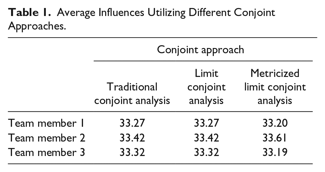
The additional spacers adjust the resulting utility values for each scenario. If this adjustment leads to the preferableness of a specific scenario, the impact of one TM changes significantly. Such a change in a TM’s influence is misleading and unwanted. Hence, the overall score at the aggregated level of all TMs’ influences should follow an equal distribution. Otherwise, MLCA includes an undesirable systematic preferableness of a specific decision maker. Thus, MLCA should not lead to a systematic preferableness on the aggregated level (Thesis 1). The MLCA part of Table 1 shows that simulated influences nearly match $33 \frac{1}{3} %$ . Again, a one-sample t test tests all variables: all mean differences fall into the 99% CI supporting Thesis 1. As a consequence, method-caused biases are no problem within this study. This finding confirms the remaining reliability of MLCA.

Nevertheless, MLCA should result in a participant’s initialized change within the influences on the individual level. Artificial participants adjust distances between previously ranked scenarios to express their perceived (instead of assumed equal) differences between these scenarios. Hence, the simulated influences utilizing the MLCA should be different to those of TCA/LCA on the individual level (Thesis 2). Table 2 shows that individual results vary between −75 and 59 utility points. Naturally, the mean value of these adjustments is zero because positive displacements balance negative ones. The resulting standard deviation underlines the large-scaled range of adjustments. Measured by the contractive assumption (i.e., the geometric distribution), these adjustments are remarkable. The absolute values of the differences as well as their mean value (7.07) and their standard deviation (5.94) emphasize this finding. Therefore, Thesis 2 finds strong support. As an example, artificial participant 2,083’s influences for the first, second, and third fictive TM change from 43%, 10%, and 47% to 36%, 18%, and 46%, which underlines the improved accuracy of MLCA. This improved accuracy of MLCA’s results is exclusively based on participant’s responses to include spacers for adjusting distances. In addition, participants do not include spacers in all cases. For example, the results of artificial participant 1,456 remain at 41% for the first fictive TM, 15% for the second fictive TM, and 44% for the third fictive TM. This artificial participant does not use any spacer. In contrast to the results of TCA/LCA in respect of the assumption of equal distances, the articulated (i.e., the simulated) unwillingness to include spacers legalizes the results of MLCA. Therefore, the MLCA has the potential to adjust utility values on the individual level. Hence, MLCA offers a better validity. The participant’s expression of opinion results in the adjustment of utility values.

Table 2.

Descriptive Statistics of TCA/LCA—MLCA Differences.

	Criteria
	Differences	Absolute value of differences
Minimal value	−75.00	0.00
Maximal value	58.57	75.00
M	0.00	7.07
SD	9.23	5.94

Note. TCA = traditional conjoint approach; LCA = limit conjoint analysis; MLCA = metricized limit conjoint analysis.

Finally, the option of adding spacers leads to a better general methodological-based applicability of the MLCA because of an additional option (confer Vermeulen et al., 2008). This argument is in accordance with generating better results due to collecting more data from each participant (Ding et al., 2009). The option of adjusting differences by positioning spacers reduces the number of cases in which the central assumption of compensatory relations is harmed (Hair et al., 2009; Riquelme & Rickards, 1992). Thus, the general applicability of MLCA should be better in comparison to TCA/LCA (Thesis 3). The applicability of conjoint analyses is equivalent to the amount of influences of 0%. TCA/LCA offer 101 artificial responses which is equal to 2%; MLCA instead offers only 23 fictive TMs with an influence of 0% which is equal to 0.5%. Hence, this decline leads to the support of Thesis 3. As an example, the artificial participant 4,673 provides influences for the first, second, and third fictive TM of 0%, 67%, and 33% for TCA/LCA. Within MLCA these numbers change to 14%, 62%, and 24% underlining the compensatory character of the first fictive TM.

Goodness of Fit and Inclusion of Correlation Coefficients

Pearson R and Kendall tau are the two important measurements for the simulation’s goodness of fit (Green & Srinivasan, 1978). First, TCA and LCA deliver a Pearson R of 0.97; this of MLCA is 0.92. Comparing these results with other studies indicates very good performing test–retest reliability (e.g., Cestre & Darmon, 1998; DeTienne, Shepherd, & De Castro, 2008). Hence, the results are very satisfactory underlining the goodness of that simulation with a high internal validity (confer Green & Srinivasan, 1978). Second, TCA/LCA leads to a Kendall tau of 0.78; this of MLCA is 0.72. As the critical value for significance at 0.05 level is a Kendall tau of 0.62 (Green, Rao, & Desarbo, 1978), both measurements are significant at 0.002 0.003 level, respectively. In accordance with prior simulation studies (e.g., Bennett & Moore, 1981; Green et al., 1978), these results are well-fitting.

In addition, I repeated this simulation study with correlation coefficients for spacers’ distributions from r = 0.1 up to r = 1.0.⁸ In all cases, the mean values of maximal values decline with rising correlation coefficients. In addition, the mean value of the difference between maximal and minimal values declines. In relation to the results of the primary simulation, these correlation coefficients lead to a smaller broadness of the results concerning Thesis 2. The maximal value of the differences between TCA/LCA and MLCA declines. Hence, both mean value and standard deviation decrease. In addition, the extent of the significant difference for Thesis 3 decreases; the main results instead are stable toward that robustness check. The most important Thesis 1 is not influenced by introducing these correlation coefficients.

Discussion

Conclusions and Implications

This study was set out to contribute to research on ETDs from a contextualized perspective in two important dimensions. First, it modifies conjoint analyses to better understand the inner structure of ETDs. This is especially important because researchers need a very accurate method to measure TMs’ influences in ETD, especially because of very limited sample sizes in this field. As these influences are, for example, an important antecedent when researching team compositions and team conflicts (confer Klotz et al., 2014), a methodological enhancement was necessary (confer especially Darmon & Rouziès, 1999; Ozer, 2007; Ulgado & Lee, 2004). Therefore, this study presents a superior alternative to direct measurements of TMs’ influences. As such, it argues that indirect decomposing measurements are superior to direct assessments (following Srinivasan, 1988). Therefore, this study is in line with literature that gathers direct and indirect methods producing different results (Louviere & Islam, 2008). Moreover, it also highlights conjoint analyses’ advantages in the context of ETDs, that is, (a) analyses on several levels, (b) access to new information, and (c) statistical power with small samples. The resulting influences of each TM are useful for a profound judgment of the respective decision, for example, by comparing individual and aggregated influences (confer, for example, de Mol et al., 2015; Kocher et al., 2006; Talaulicar et al., 2005). In a similar vein, TMs’ influences can be compared within several contexts. As an example, the predominant importance of specific TMs such as CTO, CFO, or CIO in specific decision situations can be researched in detail. In other words, researchers are enabled to open the black box of ETDs in several contexts with the help of the newly developed method.

Second, this study develops a better performing type of conjoint analysis to obtain more accurate results on the individual level. This better performance addresses the call of Short and colleagues (2010) for a methodological improvement in general and the call of Ozer (2007) for increasing the accuracy of conjoint methods in specific. The latter is in accordance with Ulgado and Lee (2004) who suggest to focus on limitations of traditional ranking-based conjoint approaches. Therefore, this study solves the well-known, but unaddressed, problem of transferring ordinal data into metric data. Due to its option of justifying distances in a comfortable way, the MLCA offers metric data for statistical calculations. Such metric data are essential for improved information content. Within the new method, a nonmetric measurement represents the starting point because of its participant-friendly nature. In addition, the MLCA offers a better general applicability. To underline the theoretical arguments, this study validates the new approach with a simulation of 45,000 assessments nested within 5,000 artificial respondents. The results clearly show that the MLCA is appropriate for measuring the influences of TMs as the individual results significantly differ from those of TCA/LCA.

To sum up, this study offers a methodological foothold for researchers to measure the influences of TMs. Through developing a new conjoint approach, this study facilitates more accurate results and enables more rigorous studies in the field of ETDs from a contextualized perspective. Therefore, this study addresses the call for developing solid measurements in the context of ETs and to explore innovative ways for collecting data (de Mol et al., 2015). The simulation part clearly shows that the MLCA delivers more accurate results on the individual level. The participant’s responses to include spacers for adjusting distances cause these differences. Hence, MLCA offers more accurate TMs’ influences compared with TCA/LCA. In addition, this study shows intense evidence for the absence of method-caused biases confirming the validity of MLCA. Therefore, researchers should use the MLCA for these specific questions instead of other conjoint methods or direct assessments of a TM’s influence. In addition, all research questions starting from an individual level depend on very accurate individual results. As the simulation part of this study shows, the MLCA offers a manageable ambiance to calculate powerful results with small sample sizes. As such, I advocate for the new approach in any conjoint study when a small sample size requires more data points from each participant (Ding et al., 2009). Figure 4 summarizes the initial idea of utilizing conjoint analysis in ETDs. Therefore, this step-by-step tutorial supports researchers in developing a suitable method for their research questions and to gain robust and accurate results.⁹

Figure 4.

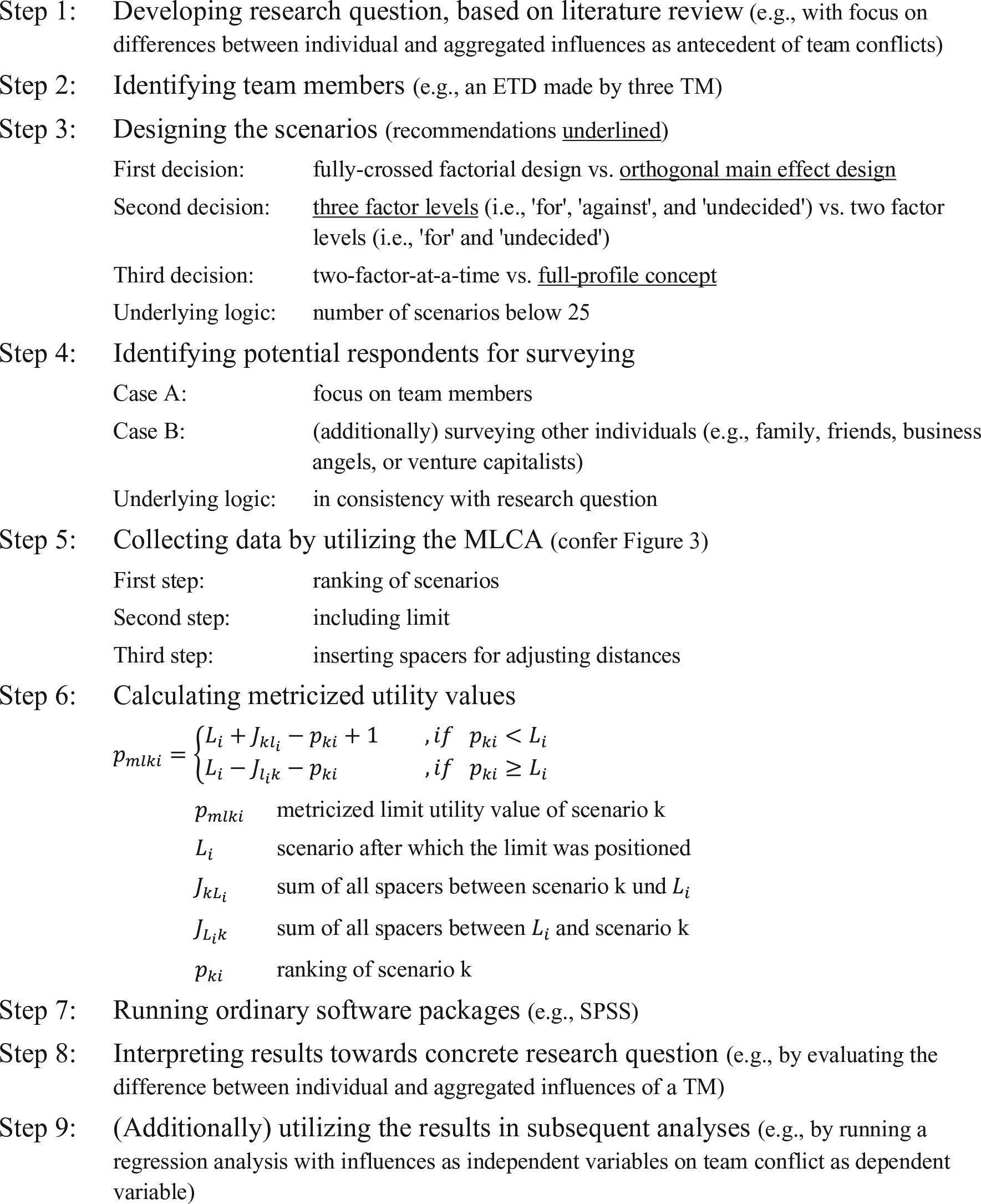
Step-by-step tutorial for utilizing the MLCA in ETDs.

Presenting an Illustrative Example

To illustrate the advantages of MLCA in practice, this study also includes the analysis of a real ET as an illustrative example. This ET consists of three TMs. To follow the general steps of MLCA, I kindly asked all three TMs (a) to rank the scenarios describing a decision situation according to the preferableness, (b) to include a limit for dividing acceptable from unacceptable scenarios, and (c) to adjust distances between ranked scenarios with spacers. For a more realistic description of the utilized scenarios, the names of all three TMs appeared on each scenario. As this pilot study was beyond a concrete research question, no specific decision situation was described. In other words, the TMs evaluated a general situation, in which, for example, two TMs are for and one TM is against proceeding. Table 3 presents the results of that experiment and subsequent calculations.

Table 3.

Illustrative Results of Analyzing an Entrepreneurial Team.

	TCA/LCA				MLCA
	Individual level			AL*	Individual level			AL*
	TM 1	TM 2	TM 3	Group	TM 1	TM 2	TM 3	Group
TM 1	44.83%	35.48%	35.48%	38.60%	41.18%	34.48%	32.20%	35.95%
TM 2	24.14%	38.71%	25.81%	29.55%	27.45%	36.21%	30.51%	31.39%
TM 3	31.03%	25.81%	38.71%	31.85%	31.37%	29.31%	37.29%	32.66%
Pearson R	.99	.99	.96	1.00	1.00	1.00	.94	.99
Kendall τ	1.00	1.00	0.94	1.00	1.00	1.00	0.94	1.00

Note. AL* = aggregated level (i.e., mean value of individual scores); TCA = traditional conjoint approach; LCA = limit conjoint analysis; MLCA = metricized limit conjoint analysis; TM = team member.

The left side of this table presents the results of the TCA/LCA with rank order positioning. Interestingly, all three TMs evaluate their own influences higher than the importance of their colleagues (indicated by relatively high values in the diagonal). Even more interestingly, especially the first TM shows a very confident evaluation of his own score (45%) leading to a high influence when considering the aggregated level (39%). In complementation, the influence of the second TM is—due to low ratings from the first TM (24%) and from the third TM (26%)—low on the aggregated level. From a consulting perspective, this difference between self-evaluated influence and external-evaluated influence would be alarming: the self-reflection of the second TM stands in contrast to the overall score—an unpleasant situation for the whole group.¹⁰

The MLCA offers adjusted and more accurate results (right side of Table 3). Both individual and aggregated results assimilate. In all cases, the influences of TMs move in the direction of more balanced values. On the group level, the influences nearly match values of totally equitable TMs. In fact, only the inclusions of spacers within the participants’ responses lead to this number. This example highlights that the new MLCA offers more accurate results on individual levels. Obviously, these more accurate results on the individual level will lead to more accurate results on the aggregated level, especially when researching small groups. These more accurate results are superior for analyzing ETDs because the differences between self-evaluated influences and external-evaluated influences are essential in that case. In fact, these influences differ to those of TCA/LCA underlining the results of the simulation part of this study. Finally, participants reported a good usability and user-friendliness of the MLCA.

Limitations

One focus of this study was to develop and test a new conjoint approach for gaining more accurate results; limitations will focus on this study’s simulation. This simulation focused on nine scenarios because this relatively small number is more manageable (Darmon & Rouziès, 1999; Green & Srinivasan, 1990). As the team size for ETDs is typically very restrictive, the required amount of scenarios will be manageable in most cases. As researchers typically report a maximum number of 25 scenarios for rank-ordering tasks (Franke, Gruber, Harhoff, & Henkel, 2006; Hair et al., 2009), most amounts of scenarios are controllable. In case of a larger amount of TMs, concentrating on two factor levels (e.g., “is for proceeding” and “is against proceeding”) reduces the amount of required scenarios.

Due to the main effect design utilized within that study, interaction effects between TMs cannot be researched. However, an additional focus of this study is to show how the MLCA can be utilized for researching ETDs. If researchers are exceedingly interested in interaction effects, utilizing a fully crossed factorial design is required. Although such a design leads to an increased number of scenarios and to decreased manageability, the procedure of MLCA remains the same. Thus, research on ETDs could indeed profit from going that route in future.

The basis for MLCA is TCA/LCA. In other words, this study does not take into account modifications of TCA (Green, Goldberg, & Montemayor, 1981; Green, Krieger, & Agarwal, 1991). However, other conjoint variants can also benefit from the initial idea of adjusting distances. As an example, researchers can integrate an additional request for evaluating distances between scenarios when utilizing a pair comparison approach. In addition, using the ranking approach does not allow integrating hold-out or replicated cards. As both enlargements are advantageous (confer Lohrke et al., 2010; Shepherd & Zacharakis, 1997), empirical researchers could integrate both modifications within a reliability part in their conjoint experiments.

Finally, a simulation study does not take into account any behavioral aspects. In fact, the core of this study is not to illustrate real TMs’ behaviors. The goal of this study is to show the reliability and better suitability of MLCA as a method for research on ETDs in several contexts. Therefore, the simulation part shows that MLCA is an appropriate method for understanding the structure of ETDs. In addition, one could discuss the simulation’s adjustments. Although the method legalizes the equal distributions of scenarios and limits, the geometric distribution is an assumption. However, this distribution is very restrictive and underlines the remarkability of the results.

Footnotes

Acknowledgements

The author thanks Dietmar Grichnik who provided general support for this research and who was a co-author of the conference submissions. Finally, the author thanks both anonymous reviewers for their valuable comments and suggestions for further strengthening this study as well as the editor Mohammad Saud Khan for his motivating and encouraging words.

Author’s Note

Prior versions of this article were presented at the Interdisciplinary European Conference on Entrepreneurship Research (IECER), at the Annual Conference of the Scientific Committee of Technology and Innovation Management, and at the Annual Interdisciplinary Entrepreneurship Conference. The author is grateful to the audience for the valuable feedback and fruitful discussions.

Declaration of Conflicting Interests

The author(s) declared no potential conflicts of interest with respect to the research, authorship, and/or publication of this article.

Funding

The author(s) received no financial support for the research, authorship, and/or publication of this article.

Notes

Author Biography

Ronny Baierl holds the professorship for Key Qualifications and is institute director of the Center for Interdisciplinary Education at the Dresden University of Applied Sciences. His work focuses in particular on issues of innovation-oriented management as well as on entrepreneurial thinking, decision-making and acting.

References

Addelman

(1962a). Orthogonal main-effect plans for asymmetrical factorial experiments. Technometrics, 4(4), 21-46.

Addelman

(1962b). Symmetrical and asymmetrical fractional factorial plans. Technometrics, 4(4), 47-58.

Amason

A. C.

Shrader

R. C.

Tompson

G. H.

(2006). Newness and novelty: Relating top management team composition to new venture performance. Journal of Business Venturing, 21, 125-148.

Andrews

R. L.

Ansari

Currim

I. S.

(2002). Hierarchical bayes versus finite mixture conjoint analysis models: A comparison of fit, prediction, and partworth recovery. Journal of Marketing Research, 39, 87-98.

Backhaus

Hillig

Wilken

(2007). Predicting purchase decisions with different conjoint analysis methods. International Journal of Market Research, 49, 341-364.

Backhaus

Wilken

Voeth

Sichtmann

(2005). An empirical comparison of methods to measure willingness to pay by examining the hypothetical bias. International Journal of Market Research, 47, 354-562.

Bao

Fern

E. F.

Sheng

(2007). Parental style and adolescent influence in family consumption decisions: An integrative approach. Journal of Business Research, 60, 672-680.

Bennett

P. D.

Moore

N. K.

(1981). Consumers’ preferences for alternative energy conservation policies: A trade-off analysis. Journal of Consumer Research, 8, 313-321.

Blaufus

Ortlieb

(2009). Is simple better? A conjoint analysis of the effects of tax complexity on employee preferences concerning company pension plans. Schmalenbach Business Review, 61, 60-83.

10.

Brinkmann

Voeth

(2007). An analysis of buying center decisions through the salesforce. Industrial Marketing Management, 36, 998-1009.

11.

Cestre

Darmon

R. Y.

(1998). Assessing consumer preferences in the context of new product diffusion. International Journal of Research in Marketing, 15, 123-135.

12.

Cochran

J. J.

Curry

D. J.

Kannan

Camm

J. D.

(2006). Conjoint optimization: An exact branch-and-bound algorithm for the share-of-choice problem. Management Science, 52, 435-447.

13.

Collins

E. G.

Guetzkow

(1964). A social psychology of group processes for decision-making. New York, NY: Wiley.

14.

Cooney

(2005). What is an entrepreneurial team? International Small Business Journal, 23, 226-235.

15.

Darmon

R. Y.

Rouziès

(1999). Internal validity of conjoint analysis under alternative measurement procedures. Journal of Business Research, 46, 67-81.

16.

Dean

M. A.

Shook

C. L.

Payne

G. T.

(2007). The past, present, and future of entrepreneurship research: Data analytic trends and training (1). Entrepreneurship Theory and Practice, 31, 601-618.

17.

De Bruyn

Liechty

J. C.

Huizingh

E. K. R. E.

Lilien

G. L

. (2008). Offering online recommendations with minimum customer input through conjoint-based decision aids. Marketing Science, 27, 443-460.

18.

de Mol

Khapova

S. N.

Elfring

. (2015). Entrepreneurial team cognition: A review. International Journal of Management Reviews, 17, 232-255.

19.

DeTienne

D. R.

Shepherd

D. A.

De Castro

J. O.

(2008). The fallacy of “only the strong survive”: The effects of extrinsic motivation on the persistence decisions for under-performing firms. Journal of Business Venturing, 23, 528-546.

20.

Dimitratos

Jones

M. V.

(2005). Future directions for international entrepreneurship research. International Business Review, 14, 119-128.

21.

Ding

Park

Y.-H.

Bradlow

E. T.

(2009). Barter markets for conjoint analysis. Management Science, 55, 1003-1017.

22.

Flurry

L. A.

Burns

A. C.

(2005). Children’s influence in purchase decisions: A social power theory approach. Journal of Business Research, 58, 593-601.

23.

Franke

Gruber

Harhoff

Henkel

(2006). What you are is what you like—Similarity biases in venture capitalists evaluations of start-up teams. Journal of Business Venturing, 21, 802-826.

24.

Franke

von Hippel

(2003). Satisfying heterogeneous user needs via innovation toolkits: The case of Apache security software. Research Policy, 32, 1199-1215.

25.

Garcia

Rummel

Hauser

(2007). Validating agent-based marketing models through conjoint analysis. Journal of Business Research, 60, 848-857.

26.

Gartner

W. B.

Shaver

K. G.

Gatewood

Katz

(1994). Finding the entrepreneur in entrepreneurship. Entrepreneurship Theory and Practice, 18(3), 5-9.

27.

Green

P. E.

Goldberg

S. M.

Montemayor

(1981). A hybrid utility estimation model for conjoint analysis. Journal of Marketing, 45(1), 33-41.

28.

Green

P. E.

Krieger

A. M.

Agarwal

M. K.

(1991). Adaptive conjoint analysis: Some caveats and suggestions. Journal of Marketing Research, 28, 215-237.

29.

Green

P. E.

Rao

V. R.

Desarbo

W. S.

(1978). Incorporating group-level similarity judgments in conjoint analysis. Journal of Consumer Research, 5, 187-193.

30.

Green

P. E.

Srinivasan

(1978). Conjoint analysis in consumer research: Issues and outlook. Journal of Consumer Research, 5, 103-122.

31.

Green

P. E.

Srinivasan

(1990). Conjoint analysis in marketing: New developments with implications for research and practice. Journal of Marketing, 54(4), 3-19.

32.

Hahn

G. J.

Shapiro

S. S.

(1966). A catalogue and computer program for the design and analysis of orthogonal symmetric and asymmetric fractional factorial experiments. Schenectady, NY: General Electric Research and Development Center.

33.

Hair

J. F.

Black

W. C.

Babin

B. J.

Anderson

R. E.

(2009). Multivariate data analysis (7th ed.). Upper Saddle River: Pearson Education.

34.

Hays

(1973). Statistics. New York, NY: Holt, Rinehart and Winston.

35.

Healey

M. P.

Vuori

Hodgkinson

G. P.

(2015). When teams agree while disagreeing: Reflexion and reflection in shared cognition. Academy of Management Review, 40, 399-422.

36.

Hong

L. J.

Liu

(2009). Simulating sensitivities of conditional value at risk. Management Science, 55, 281-293.

37.

Klotz

A. C.

Hmieleski

K. M.

Bradley

B. H.

Busenitz

L. W.

(2014). New venture teams: A review of the literature and roadmap for future research. Journal of Management, 40, 226-255.

38.

Kocher

Strauß

Sutter

(2006). Individual or team decision-making—Causes and consequences of self-selection. Games and Economic Behavior, 56, 259-270.

39.

Lohrke

F. T.

Holloway

B. B.

Woolley

T. W.

(2010). Conjoint analysis in entrepreneurship research: A review and research agenda. Organizational Research Methods, 13(1), 16-30.

40.

Louviere

J. J.

Islam

(2008). A comparison of importance weights and willingness-to-pay measures derived from choice-based conjoint, constant sum scales and best–worst scaling. Journal of Business Research, 61, 903-911.

41.

McKay

M. D.

Beckman

R. J.

Conover

W. J.

(1979). A comparison of three methods for selecting values of input variables in the analysis of output from a computer code. Technometrics, 21, 239-245.

42.

Miller

C. C.

Burke

L. M.

Glick

W. H.

(1998). Cognitive diversity among upper-echelon executives: Implications for strategic decision processes. Strategic Management Journal, 19(1), 39-58.

43.

Monsen

Patzelt

Saxton

(2010). Beyond simple utility: Incentive design and trade-offs for corporate employee-entrepreneurs. Entrepreneurship Theory and Practice, 34, 105-130.

44.

Muñoz-Bullon

Sanchez-Bueno

M. J.

Vos-Saz

(2015). Startup team contributions and new firm creation: The role of founding team experience. Entrepreneurship & Regional Development, 27, 80-105.

45.

Ang

(1999). Attribution bias: Challenges, issues, and strategies for mediation. Mediation Quarterly, 16, 377-387.

46.

Olson

D. H.

Cromwell

R. E.

Klein

D. M.

(1975). Beyond family power. In Cromwell

R. E.

Olson

D. H.

(Eds.), Power in families (pp. 235-275). New York, NY: Wiley.

47.

Oppewal

Louviere

J. J.

Timmermans

H. J. P.

(2000). Modifying conjoint methods to model managers’ reactions to business environmental trends: An application to modeling retailer reactions to sales trends. Journal of Business Research, 50, 245-257.

48.

Ozer

(2007). Reducing the demand uncertainties at the fuzzy-front-end of developing new online services. Research Policy, 36, 1372-1387.

49.

Rese

(2006). Successful and sustainable business partnerships: How to select the right partners. Industrial Marketing Management, 35, 72-82.

50.

Riquelme

Rickards

(1992). Hybrid conjoint analysis: An estimation probe in new venture decisions. Journal of Business Venturing, 7, 505-518.

51.

Schade

(2005). Dynamics, experimental economics, and entrepreneurship. The Journal of Technology Transfer, 30, 409-431.

52.

Schjoedt

Monsen

Pearson

Barnett

Chrisman

J. J.

(2013). New venture and family business teams: Understanding team formation, composition, behaviors, and performance. Entrepreneurship Theory and Practice, 37(1), 1-15.

53.

Shepherd

D. A.

Zacharakis

(1997). Conjoint analysis: A window of opportunity for entrepreneurship research. In Katz

J. A.

(Ed.), Advances in entrepreneurship, firm emergence and growth (Vol. 3, pp. 203-248). Greenwich, CT: JAI Press.

54.

Short

J. C.

Ketchen

D. J.

Combs

J. G.

Jr. Ireland

R. D.

(2010). Research methods in entrepreneurship: Opportunities and challenges. Organizational Research Methods, 13(1), 6-15.

55.

Sichtmann

Stingel

(2007). Limit conjoint analysis and Vickrey auction as methods to elicit consumers’ willingness-to-pay: An empirical comparison. European Journal of Marketing, 41, 1359-1374.

56.

Simons

Pelled

L. H.

Smith

K. A.

(1999). Making use of difference: Diversity, debate, and decision comprehensiveness in top management teams. Academy of Management Journal, 42, 662-673.

57.

Smith

Houghton

S. M.

Hood

J. N.

Ryman

J. A.

(2006). Power relationships among top managers: Does top management team power distribution matter for organizational performance? Journal of Business Research, 59, 622-629.

58.

Sprey

(1975). Family power and process: Toward a conceptual integration. In Cromwell

R. E.

Olson

D. H.

(Eds.), Power in families (pp. 61-79). New York, NY: Wiley.

59.

Srinivasan

(1988). A conjunctive-compensatory approach to the self-explication of multiattributed preferences. Decision Sciences, 19, 295-305.

60.

Srivastava

Lee

(2005). Predicting order and timing of new product moves: The role of top management in corporate entrepreneurship. Journal of Business Venturing, 20, 459-481.

61.

Stevenson

H. H.

Muzyka

D. F.

Timmons

J. A.

(1987). Venture capital in transition: A Monte-Carlo simulation of changes in investment patterns. Journal of Business Venturing, 2, 103-121.

62.

Talaulicar

Grundei

von Werder

(2005). Strategic decision making in start-ups: The effect of top management team organization and processes on speed and comprehensiveness. Journal of Business Venturing, 20, 519-541.

63.

Tetlock

P. E.

Levi

(1982). Attribution bias: On the inconclusiveness of the cognition-motivation debate. Journal of Experimental Social Psychology, 18, 68-88.

64.

Ulgado

F. M.

Lee

(2004). The effects of nationality differences on manufacturing location in the US: A conjoint analysis approach. International Business Review, 13, 503-522.

65.

Vag

(2007). Simulating changing consumer preferences: A dynamic conjoint model. Journal of Business Research, 60, 904-911.

66.

Vermeulen

Goos

Vandebroek

(2008). Models and optimal designs for conjoint choice experiments including a no-choice option. International Journal of Research in Marketing, 25, 94-109.

67.

Voeth

(1998). Limit conjoint analysis—A modification of the traditional conjoint analysis. Proceedings of the 2Th EMAC Conference Marketing Research and Practice, 7, 315-331.

68.

Voeth

(2004). Analyse multipersonaler Kaufentscheidungen mit mehrstufigen Limit Conjoint-Analysen [Analysis of multi-personal buying decisions with multilevel limit conjoint analyses]. Zeitschrift Für Betriebswirtschaft [Journal of Business Economics], 74, 719-741.

69.

Voeth

Hahn

(1998). Limit Conjoint-Analyse [Limit conjoint analysis]. Marketing ZFP—Journal of Research and Management, 20, 119-132.

70.

West

G. P.

(2007). Collective cognition: When entrepreneurial teams, not individuals, make decisions. Entrepreneurship Theory and Practice, 31, 77-102.

Understanding Entrepreneurial Team Decisions: Measuring Team Members’ Influences With The Metricized Limit Conjoint Analysis

Abstract

Keywords

Introduction

Theoretical Background

ETDs

Appropriateness of Conjoint Analyses for Researching ETDs

Developing a More Accurate Methodological Approach

Modifying TCAs for Researching ETDs

Developing the MLCA

Simulation Study for Validating the MLCA

Benefits of Artificial Data and Settings

Judgment and Findings

Goodness of Fit and Inclusion of Correlation Coefficients

Discussion

Conclusions and Implications

Presenting an Illustrative Example

Limitations

Footnotes

Acknowledgements

Author’s Note

Declaration of Conflicting Interests

Funding

Notes

Author Biography

References