
Abstract
Do people who lived through the depression take fewer financial risks because of the negative returns experienced? More generally, what is the importance of historical return streams on current investment decisions? This experiment tests this experience hypothesis and finds that subjects who experience a great crash hold, on average, 6% less of their assets in stocks than subjects who did not experience the crash, after controlling for gender, employment status, and financial literacy. Our results suggest that subjects who experience a significant market crash have lower and more volatile beliefs regarding future stock returns. Furthermore, we find that experiencing a crash causes a significant difference in the overall belief distributions between the two groups, with the crash cohort holding more realistic beliefs about future stock market returns.
Keywords
Highlights
We test whether experiencing a crash causes individuals to take fewer financial risks.
We find that subjects who experience a crash hold 6% less of their assets in stocks.
A crash results in lower and more volatile beliefs of future stock returns.
Experiencing a crash changes the entire distribution of beliefs about future returns.
A crash may result in more realistic beliefs about future stock market returns.
Introduction
The depression babies (DB) hypothesis (Malmendier & Nagel, 2011) holds that people who grew up in the depression are less willing to take financial risks because of the negative returns they experienced. Specifically, Malmendier and Nagel (2011) use econometric modeling of survey data to find that households who have experienced (were alive during) lower (higher) stock market returns report lower (higher) willingness to take financial risk and show lesser (greater) participation in the stock market. In this article, we developed an asset allocation task to directly test this hypothesis in the laboratory.
Summarizing their findings regarding an “experience effect,” Malmendier and Nagel (2011) write,
We find that households’ risk taking is strongly related to experienced returns. Households with higher experienced stock market returns express a higher willingness to take financial risk, participate more in the stock market, and, conditional on participating, invest more of their liquid assets in stocks . . . more recent experiences always receive higher weights and thus have a stronger influence on risk taking than those early in life, but even returns experienced decades earlier still have some impact . . . the estimated weighting scheme can be represented, to a good approximation, as weights that decline linearly from the most recent year down to 0 in the year of birth. Our estimates imply that young individuals, with short lifetime histories, are particularly strongly influenced by recent data. (p. 376)
The DB or experience effect hypothesis is consistent with both oral histories and historical accounts of personal experiences with long-lasting effects on individuals who lived through the Great Depression, but it seems to sit uncomfortably in the company of both standard economic theory and findings in finance. Standard models in economics and finance (the consumption capital asset pricing model (C-CAPM) and modern portfolio theory, for example) assume that agents rationally form beliefs based upon all relevant historical information and have stable risk preferences that are not affected by economic experiences, let alone economic experiences in the distant past. A number of studies in macroeconomics and finance (Boldrin, Christiano, & Fisher, 2001; Campbell & Cochrane, 1999) propose time-varying risk aversion in the very specific form of habit formation or “difference habits” models in which utility is a function of consumption minus a habit. As was the case with standard models of optimal behavior, these “habit formation” models cannot be easily reconciled with the experience effect hypothesis either. First, as stressed by Mehra and Prescott (2003), it is not clear that investors have the large time-varying fluctuations in risk aversion implied by habit formation models. Second, a large fall in wealth triggered by a large crash in asset prices should presumably lead to a fall in relative risk aversion in the short run according to habit persistence models, a proposition that is not only implausible in light of all available anecdotal evidence (phrases such as “flight to safety” or “flight to quality” are common place in the aftermath of every large crash) but also bears little, if any, connection to a long-run effect suggested by the experience effect hypothesis.
Furthermore, whenever adaptive behavior and/or expectations are allowed in economic models, more distant observations tend to carry significantly lower weight than more recent ones; for example, Malmendier and Nagel (2016) show that recent inflation experiences predict current inflation expectations. Furthermore, the representativeness heuristic and the recency effect (Hogarth & Einhorn, 1992) provide a psychological explanation for the idea that recent experiences will outweigh the influence of experiences from the distant past.
Although the recency effect suggests that judgments will be most strongly influenced by the most recent and easily available events, psychological support for a more long-run experience effect can be found in the literature on the effect of personal experiences during a person’s formative years. For example, Freud & Strachey (1966) write,
Both patients give us an impression of having been “fixated” to a particular portion of their past, as though they could not manage to free themselves from it and were for that reason alienated from the present and the future. (p. 273)
A review by Pechtel and Pizzagalli (2011) finds the early life stress can have long-lasting psychological and biological effects. Furthermore, a growing literature (e.g., Erev, Glozman, & Hertwig, 2008; Hertwig, Barron, Weber, & Erev, 2004; Nisbett & Ross, 1980; E. U. Weber, Bockenholt, Hilton, & Wallace, 1993) suggests that personally experiencing the outcome of an event has a much bigger impact on subsequent decisions especially when compared with simply reading of or learning about the focal event. Lejarraga, Woike, and Hertwig (2016) present experimental evidence to show that experiencing a market crash has a greater effect on subsequent investment behavior than simply receiving a description of the crash.
Attempts to model the influence of past events on current decisions have produced mixed results. While Malmendier and Nagel (2011) show that the influence of past events declines linearly over time, Plonsky, Teodorescu, and Erev (2015) found that a linear declining recency weight approach could be improved with a “wavy recency” model. They write, “across wide classes of dynamic binary choice environments, focusing only on experiences that followed the same sequence of outcomes preceding the current task is more effective than focusing on the most recent experiences” (p. 621). Plonsky et al. (2015) argue that agents make decisions by using past experiences that are most similar to the current choice task. Agents’ decisions are not necessarily driven by the most recent experiences but by the most recent experiences that are similar to the current environment. Wavy recency combined with the importance of early life experiences further support the hypothesis that market crashes experienced early in an investor’s life cycle can have long-lasting effects on subsequent investment decisions.
Other research on decisions from description suggests that the framing of historical information will also impact choice. Benartzi and Thaler (1995) introduced the idea of myopic loss aversion (MLA) to provide an explanation for the equity premium puzzle. MLA suggests that if investors are loss averse and evaluate their returns frequently, they will hold fewer risky assets as short-term losses will be more salient in the decision process than long-term gains. The experience effect hypothesis, as formulated by Malmendier and Nagel, and MLA are consistent in that both suggest that the recent investment returns are likely to be weighted more heavily than returns from the distant past.
In a follow-up paper on MLA, Benartzi and Thaler (1999) ran a series of experiments on repeated gambles and retirement investments. This research shows that investment choice behavior can be manipulated by changing the frame of historical returns. In an experimental survey of university employees, it was found that employees were more likely to invest in stocks if the historical distribution of returns was presented as 30-year equivalents of 1-year returns. The results suggest that investors are more likely to invest in risky assets if the historical returns are presented in a long-term frame rather than a short-term frame, thus encouraging investors to not view return streams myopically and not get trapped by recent experiences. This finding raises the possibility that experience effects may be moderated by manipulating the presentation frame of historical returns. Indeed, this moderation effect introduced by the framing of long- versus short-term returns has been found to affect investment choice in an experimental task (Sundali & Guerrero, 2009).
The interest in the empirical validity of the experience effect hypothesis is not purely theoretical. The recent financial crash of 2008 has created the possibility of a fresh new cohort of investors affected by a substantial market decline and opens up fresh questions regarding the ongoing effects of the crash on people’s risk attitudes, their beliefs concerning future stock market returns, and their rates of stock market participation. For all these reasons, we believe that a reexamination of the experience effect hypothesis can shed light on critical aspects of people’s behavior following an asset crash and in so doing can help in understanding some short- and long-run implications.
In their examination of the experience effect hypothesis, Malmendier and Nagel (2011) used repeated cross-sections of data from the Survey of Consumer Finances from 1960 to 2007. Given the limitations imposed by the data, Malmendier and Nagel (2011) could not track the decisions of the same individuals over time. A second and related limitation of the Malmendier and Nagel (2011) study also stems from the nature of the data and is related to their inability to draw causal connections between the shock (a great crash) and its impact on individual behavior. A laboratory experiment is ideally suited to address these issues and provides a natural motivation for our study.
Summarizing our laboratory study, we utilized a 2 × 2 between-subjects design with experienced returns as one factor and the framing of the historical return distribution as the other factor. The task for all subjects in the experiment was to repeatedly allocate a portfolio between two assets, one risky and the other riskless. One group of subjects (crash cohort) received returns on the risky asset that included a substantial asset crash, whereas a second group of participants did not experience this asset crash (no-crash cohort). The second factor manipulated was whether the historical returns describing the risky asset were presented to subjects in a long- or short-term frame. Two main effects were found. First, after controlling for differences in gender, age, investment experience, employment category, and other relevant determinants that could affect a subjects allocation to the risky asset, there was a significant (both economically and statistically) long-term and slowly decaying crash experience effect. Subjects whose risky asset return experience included a substantial asset crash allocated roughly 6% less of their portfolios to the risky asset than subjects who did not experience the crash, and this lower allocation was apparent 20 to 30 periods after having experienced the crash. Second, subjects who were presented with historical risky asset return information in a long-term frame invested about 5% more in the risky asset than subjects who received return information in a short-term frame.
The average allocation to the risky asset by subjects in the crash cohort at the end of the experiment was slightly below their allocation to the risky asset at the beginning of the experiment, a few periods before experiencing the crash. Although finding an overall long-term average crash effect is consistent with other experimental findings (Guerrero, Stone, & Sundali, 2012; Lejarraga et al., 2016), a novel finding in these results is that experiencing an asset crash changed the entire distribution of allocations to stocks (as opposed to just the mean allocation, as reported before). The mean, standard deviation, skewness, and kurtosis corresponding to the average allocations to stocks by the crash cohort were all significantly different from the same four moments characterizing the average distribution (probability density function) of the allocations to stocks by subjects who did not experience the crash.
As to the channels of transmission from experiencing an asset crash to stock allocations, we confirm and extend Malmendier and Nagel’s (2011) original findings. The results show that experiencing a crash leads subjects to expect that future returns on the risky asset will be lower. Furthermore, the results show that the entire distribution of beliefs regarding future risky asset returns is changed by the crash. The average distribution of beliefs of subjects in the crash cohort is significantly different from the no-crash cohort in its four moments (mean, standard deviation, skewness, and kurtosis) and also different from the underlying objective probability distribution of stock market returns of the Dow Jones Industrial Average (DJIA), the market index used in our study. Of particular interest is the result involving the tails of the three distributions. The left tail of the probability density function corresponding to the crash cohort is significantly “fatter” than the one corresponding to the no-crash cohort, but not quite as fat as the objective distribution of returns represented by the DJIA. The crash versus no-crash comparison suggests that crash cohort subjects become more realistic in their appraisal of the likelihood of extreme negative shocks. The crash versus DJIA comparison suggests that people underweight the true objective probability of an extreme negative event, even after experiencing it, a finding that is in line with the literature on rare events (Camilleri & Newell, 2011; Erev et al., 2008; Hertwig et al., 2004; Rakow & Newell, 2010).
The rest of the article is organized as follows. Section 2 describes the experimental design and procedures. Section 3 presents demographic statistics on the sample pool and uses ANOVA techniques to identify between condition effects. Section 4 builds a series of multivariate regression models designed to disentangle the DB’s effect from other independent influences on influencing the share of the risky asset held by subjects. Section 5 considers the transmission mechanisms that may account for the finding of lower allocations to the risky asset in the crash cohort. Specifically, analyses are presented that support the finding that subjects’ beliefs regarding expected future returns on stocks are driving the main results over the competing hypothesis of a long-term change in risk aversion. Section 6 concludes with a discussion of the results and suggestions for future research.
Experimental Design and Procedures
Experimental Design
The experimental design is a 2 × 2 between-subject design. The first manipulation varies how long subjects make asset allocation decisions and the return stream that subjects experience. Subjects make allocation decisions for 20 or 40 years and receive the return stream of the DJIA from either 1945-1964 (20-year cohort) or from 1925-1964 (40-year cohort). The actual return stream on the DJIA from 1925 to 1964 is shown in Table 1. Subjects in the 40-year condition will experience the return stream crash on the DJIA from 1929-1932.
Actual Return on DJIA 1925-1964.
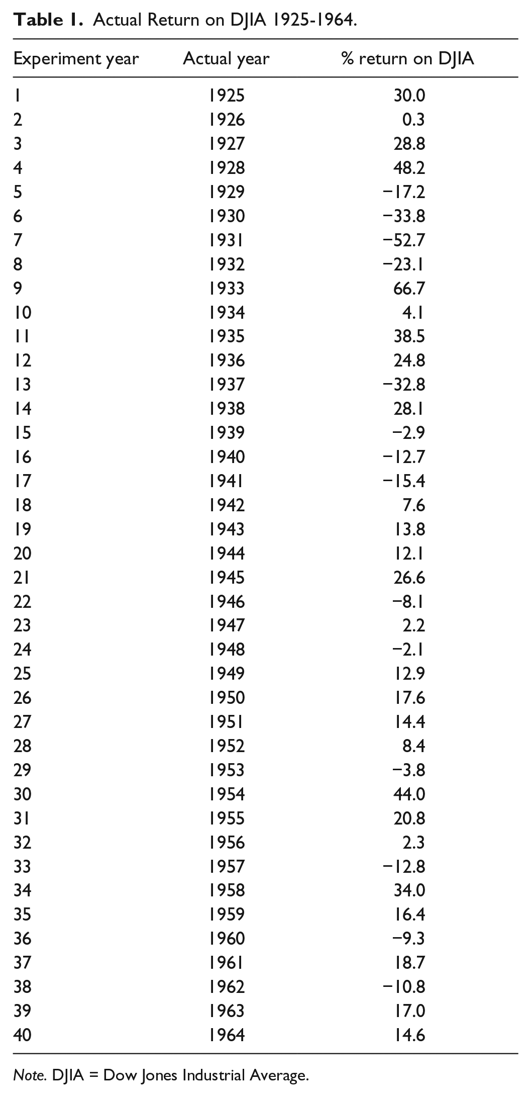
Note. DJIA = Dow Jones Industrial Average.
The second manipulation varies the display of the distribution of the risky asset performance between short- and long-term frames (see Figure 2). Subjects in the short-term frame only receive the statistical summary information (mean, standard deviation, maximum, minimum) on the DJIA from 1898-2011 while subjects in the long-term frame receive a column graph showing the full distribution of the DJIA annual percentage returns. The long-term frame presentation is a simple graphical summary (a histogram of the DJIA returns ordered from lowest to highest) designed to show subjects that over the long term the DJIA is a good investment. The experimental design is shown in Table 2 and the experimental task is described in more detail in “Experimental Task” section.
Experimental Design.

Note. DJIA = Dow Jones Industrial Average.
The logic underlying this experimental design is to better understand how asset allocation decisions are impacted by the return experience and, simultaneously, by the return description. While on the one hand the design is a fairly direct experimental test of the crash experience hypothesis, the 2 × 2 design is also a modest attempt to address the issue of personal experiences versus return description. We hypothesize that subjects will be affected by both the return experience and the return description. Our hypotheses for this experimental design are summarized below:
Procedures
Recruitment was conducted by sending a flyer in the campus mail to all (approximately 1,400) University of Nevada, Reno (UNR) faculty and staff employees. The flyer stated that a 1-hr experiment on investment decision making was taking place and a subject could earn between US$5.00 and US$50.00 depending upon performance. Eighty subjects signed up to participate.
The experiment was conducted at the UNR in a computer lab in the College of Business. The laboratory has eight rows of networked personal computer stations with six computers in each row. The subjects who participated in each condition were placed so that they could not see the computer of another subject and would have privacy to make their decisions. When subjects arrived, they sat down at a computer station and could begin reading the consent form and instructions and filling out the Domain-Specific Risk-Taking (DOSPERT) risk attitude questionnaire. The consent forms were then read aloud and after consent was obtained each subject received a US$5.00 show-up fee. As the recruitment flyer stated that subjects would receive a minimum compensation of US$5.00, the show-up fee was given to fulfill this promise. Subjects were then told that any further compensation in the experiment was contingent on their performance in an asset allocation task.
After all the instructions were read and questions answered, the subjects then made two practice decisions for which they were not paid. Each subject then proceeded at his or her own pace through the experimental tasks. Most subjects took between 30 and 45 min to make all of their decisions. After all the decisions were completed, each subject filled out a second DOSPERT scale questionnaire, a demographic questionnaire and a receipt documenting their earnings. Each subject then walked to the back of the room where they were paid individually and anonymously in cash for their performance, thanked, and dismissed from the laboratory.
Due to a technical problem in data collection, data for two of the subjects were not complete. This excluded one subject in the 40-year short-term condition and one subject in the 40-year long-term condition, and resulted in a total of 78 subjects.
Experimental Task
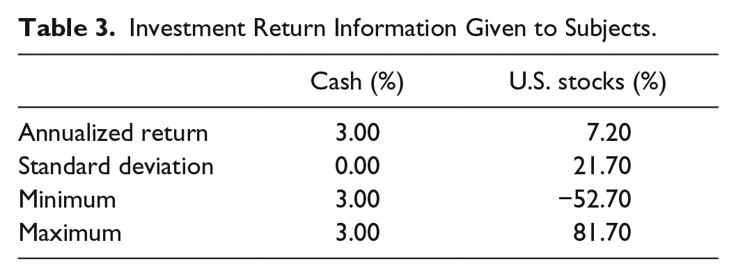
The basic experimental task was designed to have subjects make the type of repeated asset allocation decisions that an investor might have to make when managing an endowment of money over a long period of time (e.g., investing for retirement). The constructed task for subjects in the experiment was to allocate an endowment of money across two investment options, cash and stock. Table 3 below provides the information given to subjects regarding the investments and potential return on the assets in the experiment. Subjects were told the stock asset was a large cap mutual fund with returns similar to those of the DJIA. Subjects were told to expect that the returns on the stock asset would be similar to what the DJIA produced in the time period of 1898-2011.
Investment Return Information Given to Subjects.
Prior to making their asset allocation decisions, subjects were asked to provide a forecast regarding the percentage return on the stock asset in the next period. To motivate the subject to give an accurate estimate of the expected return on stocks, each subject was paid US$0.25 if the estimate was within plus or minus 10% of the actual return. A subject entered his forecast regarding the return of the stock asset for the next year on the spreadsheet shown in Figure 1. On this spreadsheet the subject was given performance feedback regarding her estimate from the prior year, information regarding the historical distribution of returns on the DJIA from 1898-2011, and then asked to make an estimate for the next year. Subjects in the Long-Term frame condition were shown a table and graph regarding the distribution of DJIA returns on the worksheet (Figure 2); subjects in the Short-Term frame were not shown the table or the graph of the distribution of DJIA returns on the worksheet and only had the information presented in Table 3 in the subject instructions. This manipulation is in line with prior literature that has found that representation matters as the same statistical information may be mathematically equivalent but may not processed by the human brain as equivalent objects (Gottlieb, Weiss, & Chapman, 2007; Hertwig, Barron, Weber, & Erev, 2006; Rakow & Newell, 2010).

Subject interface for entering estimate of stock returns.

Information regarding return on stock investment provided to subjects in long-term condition only.
After a subject provided her forecast on the stock asset for the next year, the subject would begin making her asset allocation decisions using the spreadsheet interface as seen in Figure 3. Each subject was given a US$3.00 endowment to begin the experiment. Each “year,” the subject chose how to invest their endowment. The subjects had two investment choices: U.S. stocks (US) and cash (C). To make an asset allocation decision, a subject would enter a number in the appropriate cell for a chosen investment. For example, if a subject chose to allocate ½ of her funds to stocks and ½ to cash, she would enter 50 in the Asset Allocation Column for U.S. stocks and 50 in the column for cash. The spreadsheet also displayed the portfolio expected return and standard deviation based upon the historical distribution of returns on the DJIA from 1898-2011. The layout of the asset allocation interface was identical across all conditions of the experiment. The spreadsheet was built with checks and controls to insure accuracy in decision entry. Once a subject was satisfied with his or her asset allocation decisions for a particular year, she would then click a “final decision” button on the spreadsheet and the investment returns for that year would be displayed and the cumulative account balance was updated. After beginning Year 1 with a US$3.00 endowment, each year after that a subject’s account balance rose or fell depending upon the yearly performance of their portfolio.

Subject interface for entering asset allocation decisions.
A sample feedback spreadsheet is shown in Figure 4. In the Long-Term condition, the feedback given to a subject only included the performance results from the prior year. In the Short-Term condition, the feedback given to a subject included all the performance results from all the prior years completed thus far. This difference in the framing of the feedback results was designed to give the subjects in the Short-Term conditions the opportunity to look for patterns in the return stream. The idea for displaying performance feedback in this manner comes from how many casinos have chosen to display past winning numbers in the game of roulette (Sundali, Safford, & Croson, 2012). After a subject finished reviewing the results, he or she would then click a button to begin making her estimate regarding the return on stocks for the next year. Subjects continued making decisions in this manner for 20 or 40 years and were paid the cumulative amount earned in their portfolio at the end of the experiment.

Subject interface results page.
To measure risk attitudes and risk aversion, subjects were asked to fill out two DOSPERT scale questionnaires, one prior to the asset allocation task and one after completing the task. The DOSPERT scale (Blais & Weber, 2006) provides a validated scale for measuring a person’s risk attitudes and serves as a proxy for risk aversion. The scale includes a total of 30 items in five risk domains: ethical, financial, health/safety, recreational, and social. Examples include riding a motorcycle without a helmet (health/safety) and betting a day’s income at a high-stake poker game (financial). Subjects rated each item on the scale from 1 to 7 based on the likelihood they would engage in the activity/behavior (1 = extremely unlikely, 7 = extremely likely), the perceived risk of the activity (1 = not at all risky, 7 = extremely risky), and the expected benefit of the activity (1 = no benefits at all, 7 = great benefits). The pre-/post-collection of the DOSPERT scale allows for the measurement of each subject’s risk perception prior to the asset allocation task and to measure any change in risk perception or attitude that occurs due to the experiment.
Results
Sample Demographics
Seventy-eight subjects participated in the experiment and the subject pool was 45% male and 55% female. The average age of participants was 27.4 years, with 51% in the 18 to 22 age bracket, 23% in the 23 to 29 age bracket, 19% in the 30 to 49 age bracket, and 6% were 50 years or older. In all, 24% reported being either university staff or faculty employees, and 73% were currently students. Each subject was asked to self-report on how much experience he or she had with investment decisions similar to those in the experiment. On a 1 to 7 scale (1 = none at all, 7 = a great deal), the average response to this investment experience question was 2.5, with 65% answering 1 or 2; 29% answering 3, 4, or 5; and 5% answering above 5. The average subject payment was US$22.11.
ANOVA Tests for Condition Effects
The average allocation to stocks across all conditions is 53.4%. As seen in Figure 5 and Table 4, in the Short-Term condition, the allocation to stocks is 51% compared with 56% in the Long-Term condition. The average allocation to stocks declines from 57% in the 20-year condition to 52% in the 40-year condition. A repeated measure ANOVA (using the Proc Mixed procedure in SAS) confirms a statistically significant main effect for Frame (Short vs. Long; F = 4.66, p < .02) and for Cohort (20 year/40 year; F = 3.66, p < .056). The Frame × Cohort interaction effect is not significant. The Framing manipulation leads subjects in the Short-Term frame to allocate less to stocks. The Cohort manipulation shows that subjects who experienced the market crash in the 1930s allocate less to stocks than subjects who do not experience the crash.

Asset allocation to stocks across conditions.
Average Allocation to Stocks by Condition.
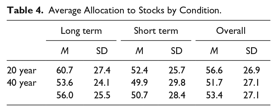
Figure 6 plots the allocation to stocks by year (averaged over 5-year blocks) and by cohort (20/40). As seen in Figure 6, subjects in both cohorts began by allocating about 57% to 58% to stocks in the first 5-year block. Subjects in the 40-year cohort reduced the allocation to stocks to a low of 47% in the second 5-year block. The allocation to stocks by subjects in the 40-year cohort was below the allocations of the 20-year cohort in each of the last four blocks of the experiments. A repeated measure ANOVA confirms a statistically significant interaction effect for Cohort (20 year/40 year) by the repeated measure Year (F = 2.4, p < .01).
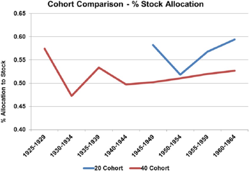
Asset allocation to stocks by 5-year block and cohort.
Multivariate Regression Analyses
We next present a series of multivariate regression analyses. As seen in Column 1 of Table 5, we begin with a simple ordinary least squares (OLS) specification in which the share of stocks is the dependent variable and the explanatory variables are a dummy variable for Gender (female = 1; male = 0), a dummy variable for Student (UNR student = 1; UNR faculty/staff = 0), an indicator variable for subjects’ self-reported investment experience (Investment Experience takes discrete values ranging from 1 to 7, with higher numbers associated with higher experience), and a dummy variable for the Crash cohort (1 = 40-year crash cohort, 0 = 20-year no-crash cohort). The Crash cohort dummy captures if the allocation to stocks is different between the crash and no-crash cohorts after controlling for observable characteristics that have been shown to influence risk attitudes and, by implication, the choice of stocks (Croson & Gneezy, 2009). The age of subjects was not included in the regressions because it proxies for and is highly correlated with investment experience. As a simple way to avoid the time dependency created by repeated decisions on contiguous observations (or even perhaps among small blocks of observations), all variables were averaged over 10-year periods, yielding one observation per decade for each subject, for a total of four observations per subject for subjects in the 40-year cohort, and two observations per subject for subjects in the 20-year cohort.
Regression Analysis.

Note. OLS = ordinary least squares. UNR = University of Nevada, Reno.
The crash cohort dummy variable is negative and statistically significant (p < .01) indicating that the 40-year cohort holds six percentage points less in stocks than the 20-year cohort, after controlling for observable characteristics such as gender, investment experience, employment status, and so on.
The next regression in Column 2 of Table 5 attempts to isolate the long-term effect of the crash. To begin, we drop the first 20 years of decisions from the 40-year cohort. Both cohorts are thus left with 20 years of data each for analysis. By concentrating on the last 20 years of data for the 40-year cohort, coefficient estimates cannot, by definition, be contaminated by short-term effects. The OLS models in Columns 1 and 2 of Table 5 are thus the same specifications but with the sample restricted to the years 1945-1964 for both cohorts. In other words, the crash years from 1925-1944 are dropped for the crash cohort.
The results in Column 2 are very similar to those in Column 1 when the full sample was used. The estimated coefficient associated with the Crash dummy remains in the same quantitative ballpark and is also statistically significant at the 1% level. The remaining coefficients are also stable quantitatively.
Transmission Mechanisms
An important finding from the experiment is that experiencing the stock returns during the great depression lead the 40-year cohort to allocate less to stocks compared with the 20-year cohort that did not experience these depressed returns. We now investigate some factors that could be accounting for this result. In their DB paper, Malmendier and Nagel (2011) suggested that the reduced risk taking they found in their sample could be due to either a permanent increase in risk aversion or a change in the beliefs regarding future stock market returns. We address these hypotheses next.
Risk Attitudes and Risk Aversion
To measure risk attitudes, a subject filled out the DOSPERT questionnaire developed by Blais and Weber (2006) before and after the asset allocation task. The DOSPERT questionnaire measures domain-specific risk attitudes and serves as a proxy for risk aversion. The results of our analyses on the overall risk attitude, as well as the financial risk attitude, of the crash cohort were not significantly different from the noncrash cohort either before or after the asset allocation task.
These results weaken the argument that a change in risk aversion can account for the differences in asset allocation across cohorts. Not only is there no difference in risk attitudes across cohorts but the analyses show that there is a decrease in risk aversion from pre- to post-survey measures for all subjects. It is difficult to reconcile lower reported risk aversion with lower allocations to the stock investment.
Beliefs About Future Stock Market Returns
As explained in “Experimental Task” section, each year a subject was asked to estimate what she thought the percentage return on the stock investment would be in the next year. If the subject’s guess was with +/–10% of the actual return, the subject received US$0.25 for their guess. Given the information presented to subjects regarding the historical returns on the DJIA and the instructions that future returns in the experiment would be similar to the historical distribution, a rational subject should forecast that the return on the stock investment in each year of the experiment would be equal to the mean of the historical distribution or an expected return of 7.2%. If the market crash does have an effect on subject beliefs then we would expect that effect to be negative and subjects in the 40 cohort should forecast lower future returns compared with subjects in the 20 cohort.
We begin the analysis of beliefs by examining the correlation between stock allocations and the expected return on stocks. Figure 7 shows the average allocation and expected returns average by 5-year blocks by cohort. The correlation between expected returns and stock allocations is 0.89 in the 40 cohort and 0.99 in the 20 cohort. The high correlation suggests that there is strong connection between beliefs and allocations.

Stock allocations and beliefs in 20- and 40-year cohorts.
Next, the belief and risk attitude measures were added to the regressions reported in Table 5. Recall that the variables in these regressions were averaged over 10-year blocks to avoid the time dependency created by repeated decisions on contiguous observations. As seen in Column 3 of Table 5, the coefficient for the Beliefs variable is positive and significant, suggesting that as the belief about the expected return on the stock asset goes up, so does the current year stock allocation. The Risk Attitude variable is not statistically significant.
A series of additional regressions were conducted on a data set that was not averaged across blocks to control for the repeated measures issues. The dependent variable in the regression remained the allocation to stocks in each year of the experiment. The explanatory variables included the subject’s stock allocation lagged 1 year; the actual return on the stock asset lagged 1, 2, and 3 years; the subject’s belief regarding the expected return on the stock asset in the next year; a dummy variable if the subject was in the crash cohort; and the demographic variables of faculty/staff, student, and investment experience. In the full regression with all of the explanatory variables above, all of the variables were statically significant (at p < .01) except for the faculty/staff and student dummy variables. As expected, a subject’s current stock allocation was highly correlated with their allocation in the prior year. Also, a subject’s current stock allocation was higher if there was a positive return on the stock asset in the prior year; but, the higher the return on the stock asset lagged 2 and 3 years, the lower current stock allocations. Finally, the Belief and Crash cohort variables remained significant and quantitatively consistent even after controlling for these other variables. We continue our analysis of the Belief variable in the next section.
Comparison of belief distributions between cohorts
In Table 6, we report the characteristics for subject beliefs across the 20 and 40 cohorts in terms of mean, standard deviation, skewness, and kurtosis statistics. Apart from the differences in means already discussed in the previous section, there was also quite a range in the distribution of subjects’ beliefs with only a very few subjects providing a stable point estimate of 7.2%.
Belief Distribution Characteristics.

The standard deviations show a slightly higher volatility of beliefs for the crash cohort (15% vs. 13%) for the whole sample. Interestingly, the standard deviation declines slightly (from 16% to 13%) in the last years of the experiment for the crash cohort. Furthermore, the volatility declines in the last 20 years of the experiment for the crash cohort, moving in the wrong direction in terms of what would be expected if learning from experience is at play.
The Skewness statistics of 2.09 and 0.77 on the distributions of the 20 and 40 cohorts respectively indicate the distributions were right skewed suggesting optimistic beliefs regarding future stock returns, confirming the findings reported in the previous section in regard to the mean statistic.
The Kurtosis statistics of 9.14 and 4.81 on the 20 and 40 cohort distributions suggests both had very sharp peaks around the mean. The sharp peaks in the distributions are likely explained by the incentive systems for guessing stock returns that encourage a mean point estimate of 7.2%.
There are some interesting differences in the distribution of beliefs between the cohorts. First, the skewness and kurtosis statistics are both lower in the 40-year cohort (Crash cohort) compared with the 20-year (noncrash) cohort. As seen in Figure 8, the 20 cohort had a more peaked distribution around the mean and thinner tails. Fatter tails in the 40 cohort suggests that subjects in this group were more likely to provide very high or low estimates regarding future stock returns. The fatter tails are more pronounced on the negative side of the distribution, confirming that the 40-year cohort placed a higher probability on large negative stock returns than the 20-year cohort.

20-year versus 40-year cohorts (full sample).
Using the Kolmogorov–Smirnov (KS) to test for differences between distributions, there is a significant difference in the belief distribution between the 20- and 40-year cohorts (D = 0.28, p < .01). This difference in the distributions of beliefs between cohorts suggests that once subjects in the 40-year cohort actually experienced a stock market crash and recovery, they were then more cognizant that large (primarily) negative returns were possible and were more likely to forecast large (mostly) negative returns in the next year.
To validate this finding, we performed further KS tests on the distributions of beliefs. Within the 40-year cohort, we find a significant difference in the distribution of beliefs between Years 1 to 5 and Years 6 to 40 (D = 0.14, p < .01). Subjects in the 40-year cohort began the experiment with very optimistic beliefs (mean stock estimate = 14.1% in Years 1 to 5) and a peaked distribution (Kurtosis = 8.67). As seen in Figure 9, the tails of the distributions for Years 6 to 40 are fatter than those in Years 1 to 5. These findings suggest that although the 40-year cohort began the experiment with very optimistic beliefs, these beliefs were significantly adjusted after experiencing the crash. Interestingly, we find no significant difference in the distribution of beliefs between Years 1 to 20 and Years 21 to 40 (D = 0.05, p < .22) for the 40 cohort. Taken together, these findings suggest that the crash caused beliefs to change quickly and that these changes remained consistent across the later years of the experiment.

Fourty-year cohort, first 5 years (1-5) versus last 35 years (6-40).
A second piece of evidence regarding the impact of the crash is related to the significant statistical difference in the distribution of beliefs for the Years 21 to 40 between Cohorts 20 and 40 (D = 0.08, p < .05). As the return stream that the cohorts experienced in Years 21 to 40 was identical, this is further evidence that it was the experience of the crash that led to the change in beliefs of the 40 cohort.
In Figure 10, the cumulative distribution functions of the actual annual returns from the DJIA and the distributions of beliefs for the last 20 years of the 20 and 40 cohorts are stacked on top of each other. It is interesting to note that the distribution of beliefs from the 40-year cohort more closely resemble the actual distribution of returns on the DJIA than does the distribution from the 20-year cohort. This suggests that there is a learning process occurring in this experiment in regard to the overall distribution of beliefs, and that after experiencing the crash the 40-year cohort has more realistic beliefs about future stock market returns. Still, it is clear from Figure 10 that that the process is incomplete and the 40-year cohort significantly underestimates the true probability of a crash, a finding that is in line with a recent and rapidly growing literature on rare events in the field of psychology (Hertwig et al., 2004).
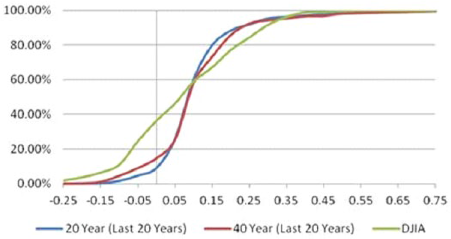
Cumulative distribution functions for last 20 years versus DJIA.
Belief Modeling
We conclude our analyses by individually modeling the weight structure of stock returns that best explains each subject’s stock allocations. We follow Hertwig et al. (2006) and assess how much weight prior stock returns should be given in predicting current allocations for each individual in the Crash cohort. Some weight structures put more weight on the stock returns of the most recent periods while others put more weight on the stock returns of more distant periods.
Hertwig et al. (2006, p. 85) propose that the weight of each return should be given by:

where t refers to the time elapsed from the midpoint of the 4-year period crash, and the parameter gamma in the power function can be either positive or negative, thus governing the curvature of the function, and thus determining if more weight is imposed to the early or the late returns. When gamma is positive, more recent returns receive more weight. When gamma is negative, more distant returns receive more weight, as shown in Figure 11.
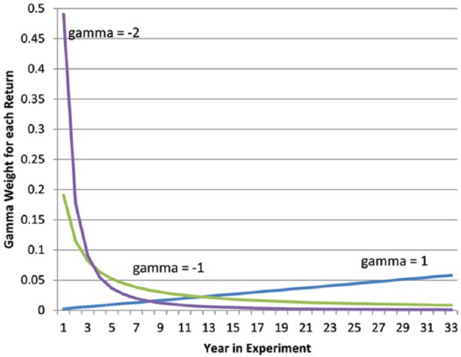
Sample of memory weights.
We then run regressions for each individual in the Crash cohort in which the dependent variable is Stock allocation (% allocated to stocks) and the explanatory variables include the subject’s beliefs and the (alternative) weighted stock returns. The gamma parameters that were tested as alternatives for the best fit in each regression were the following: gamma = 1/5, 1/2, 1, 2, 5, –1/2, –1/5, –1, –2, –5. Regressions were run for each individual’s allocations for each of these parameters.
The regressions for each individual and each weight structure were of the following form:

where s denotes stock allocation, i refers to each individual in the treatment (Crash) group, j refers to each weighted (stock) return structure, h refers to the treatment group, and r(t) refers to the (unweighted) stock returns faced by the treatment group in each year of the experiment, and belief(t) denotes the self-reported, incentivized belief reported by every subject prior to making their stock allocation decision.
The regression with the highest t statistic for a given weighted return structure was then chosen as the one that best fit each individual’s behavior. In that way, we attempted to identify subjects that put more weight on the stock returns that occurred early in the experiment or the distant past, as opposed to subjects that put more weight on the most recent returns.
Table 7 below shows the distribution of individuals in the treatment group according to the pattern of weighted returns that best explained their stock allocations.
Best Fit Weight For Each Subject in Crash Cohort.

As Table 7 shows, for 11 of 39 individuals in the treatment group, the weighted return structure that best fit their stock allocations had a negative gamma parameter (i.e., those associated with putting weight on more distant returns). Five out of 39 individuals in the treatment group had stock allocations that can best be explained by weighted returns in which recent returns receive more weight than distant returns; that is, the best fit was obtained with a positive gamma parameter, suggesting the existence of a recency effect, in spite of the experimental manipulation exposing them to a large salient, early crash. One individual (id 118) displayed the same constant allocation to stocks during the 40 experimental “years.” A significant number of individuals in the treatment group (22/39) kept their stock allocations unchanged for prolonged periods, leaving very little variation to be explained by any pattern of returns (adjusted or otherwise), making it impossible to identify the optimal structure of weights (those are represented in the column “No discernible pattern” at the far right of Table 7).
Conclusion
This study examines how the experience of an asset crash and the description of historical asset returns affect subjects’ asset allocations. Our findings include (a) subjects who experience a market crash allocate about 6% less to the risky stock investment compared with subjects who do not experience the crash after controlling for other explanatory variables; (b) subjects who receive a description of historical returns with a long-term frame orientation invest about 6% more in the stock asset; (c) the long-term framing of historical asset returns does not compensate for the effect of a significant crash early in the investment life cycle; (d) our best explanation for the lower stock investment allocations of the crash cohort is that these subjects have more volatile and pessimistic beliefs regarding future stock returns and that the reduced risk taking is not attributable to an increase in risk aversion; (e) experiencing a market crash increases the belief and expectancy that another market crash is possible; and (f) the impact of the distant experiences effect is seen most clearly in years following negative returns on the risky asset.
Recently there have been several studies examining how investors react to significant market declines. Malmendier and Nagel (2011) used data from the Survey of Consumer Finance to examine the risk-taking behavior of respondents who lived through the Great Depression. M. Weber, Weber, and Nosić (2012) used survey data from Barclays online broker customers to examine the hypothetical risk-taking behavior of respondents from September 2008 to June 2009, a period of another market crash.
Our study presents a controlled experimental study with financial incentives to examine the risk-taking behavior of subjects exposed to the market returns from the Great Depressions and compares these subjects with a control group not exposed to the returns from the Great Depression. As all three studies employed very different methodologies, a comparison of the similar findings between the three papers provides an important contribution to the literature.
One of the most interesting similarities between the three studies is that all three report a decline in risk taking in the range of 6% to 10% following exposure to significant asset/market declines. Malmendier and Nagel’s (2011) models estimate that an increase of 5% of experienced real stock returns is associated with an increase of about 7% in the percentage of liquid assets allocated to stocks. M. Weber et al. (2012) report that the mean percentage invested into a hypothetical risky portfolio by Barclays survey respondents fell from 56% to 47% from September of 2008 to March of 2009, a period during which the U.K. stock market (FTSE-All Share) fell by about 30% and then fully recovered those losses. Our experimental results show that the crash cohort allocated about 6% less to stocks compared with the noncrash cohort. The average annual return on the DJIA for the crash cohort was 7.9% versus 10.1% for the noncrash cohort. The tentative conclusion to draw from these converging results is that on average a significant market crash leads to about a 6% to 10% reduction in portfolio allocation to the risky asset in both the short and long term by individual investors.
A second tentative conclusion to draw from the comparison of the three studies is that the transmission mechanism causing the reduction in risk taking following market crashes appears to be changes in investors’ beliefs and expectations regarding future market returns rather than a change in investor risk aversion or risk attitude. Malmendier and Nagel (2011) conclude, “We also offer some evidence that experience influences risk taking, at least partly, by affecting beliefs rather than risk preferences. We show that higher experienced stock returns are associated with more optimistic beliefs about future stock returns” (p. 410). Our experimental results suggest that beliefs and asset allocations are highly correlated, that risk aversion does not increase after experiencing an asset crash, and that the beliefs and allocations of subjects in the crash cohort are very pessimistic in the face of any declines on the risky asset. M. Weber et al. (2012) find that self-reported measures of risk attitudes were stable over time in a repeated longitudinal survey and that subjective measures of risk and return expectations are highly correlated with risk-taking behavior. Thus, all three studies lend support for the hypothesis that changes in risk-taking behavior following asset/market crashes can be attributed to changes in beliefs regarding future returns rather than changes in risk attitudes or risk aversion.
Discussion
Rare events, by definition, happen rarely. Buying the winning lottery ticket, losing a cherished career job, dating our favorite movie star, or being caught in a once-in-a-lifetime natural disaster are all things that very few of us ever experience. The description of some rare events capture our imagination and lead us to overestimate their true probability of occurrence. Highly emotional events, such as terrorist attacks (Sunstein, 2003), are often significantly overweighted. For example, the fear of terrorism results from an availability cascade whereby vivid images of cruel, violent deaths are reinforced by media attention and social interactions, inducing easy access and retrieval of those mental images and this induced emotional arousal leads to a significant overestimation of the likelihood of the event (Sunstein, 2002; Slovic, Finucane, Peters, & MacGregor, 2004).
But for the majority of experienced rare events, as opposed to those presented by description, the underweighting of the true probabilities is the typical finding in the literature, especially for feedback-type studies, such as ours. This article confirms that finding, and is consistent with the findings of Lejarraga et al. (2016). Both cohorts in our experiment received descriptive written information about the historical distribution of stock market returns and were told that the actual returns to be experienced during the experiment were likely to be similar to the historical ones (an incomplete description of the risky prospects). Even so, both cohorts greatly underweighted the true probability of large negative returns. Yet the crash cohort underweighted the true probability of a crash by a lesser amount and also showed signs of learning from the experience of a crash.
The crash that subjects experienced only lasted a few periods, but it seemed to have a long-term effect on subjects’ asset allocations. As the crash in the experiments was relatively short, the impact of the crash seems to have more to do with the intensity (or depth) of the crash rather than the length, a finding in line with literature on peak-end rules and duration neglect (Fredrickson & Kahneman, 1993; Kahneman, Fredrickson, Schreiber, & Redelmeier, 1993). Salience is perceived according to the magnitude of the event but recalled according to the intensity of the event at its peak and at the end of the episode, especially in the case of bad events (Kahneman et al., 1993). Indeed, there is evidence of “duration neglect,” a phenomenon by which the total amount of discomfort or pain brought about by the bad event is erroneously recalled and discounted if the episode finishes on a somewhat good note (Fredrickson & Kahneman, 1993).
Future research on this topic should consider the following issues. First, while the evidence we reported in this experiment clearly leans toward the explanation that beliefs regarding future market returns are driving the lower asset allocations rather than any changes in risk aversion, we suggest that a research design that allows for the capturing of time-varying measures of risk aversion between asset allocation decisions would be informative. Second, our results suggest that the description versus experience component of the experiment is a critical factor in the results and further thought on this distinction is warranted.
Finally, further research is necessary to further assess the importance of the primacy and recency of stock returns on current allocations. Malmendier and Nagel’s (2011) experience effect model suggests that memories of a crash fade in an approximately linear fashion. Thus, if you recently experienced a crash it will have a significant effect on your current allocations but if the crash was in the distant past, or if you are young and have no experience with a market crash, then crash returns will have little influence on your current allocations. Our experimental work suggests that for a significant number of subjects the memory of a crash is fairly long lived and can lead subjects to hold less of the risky asset many periods after the crash. Unfortunately, the number of periods and absolute amount of time in our experiment is probably not long enough to formally assess the relative importance of recent versus distant events. A longer experiment with hundreds of decision periods along the lines of Plonsky et al. (2015) may be a better model to answer questions about the relative importance of recent versus distant events. In addition, an allocation experiment with hundreds of periods would also be better able to assess the importance of “wavy recency” or whether patterns of prior returns lead to an expectation that another crash is coming. Whether it is done in the lab or the field, one goal of future work should be to sort out the effects of primacy and recency on investor behavior in an environment where the investor experiences assets booms and busts. As asset markets are likely to continue to boom and bust on a regular basis, a clear understanding of how investors behave in such environments is necessary to provide tangible advice on how to best avoid costly investment mistakes.
Footnotes
Acknowledgements
The authors wish to thank participants at the 2012 Bay Area Behavioral Economics Workshop, discussants at the 2012 Academy of Behavioral Finance Conference, the University of Nevada, Reno brown bag seminar series, and especially Stefan Zeisberger and Gabriele M. Lepori for helpful comments and suggestions on this article. We also thank two anonymous referees for their comments and suggestions, which greatly improved the manuscript. Any remaining errors are our own.
Authors’ Note
This article is based on research completed for Amanda Safford’s dissertation.
Declaration of Conflicting Interests
The author(s) declared no potential conflicts of interest with respect to the research, authorship, and/or publication of this article.
Funding
The author(s) received no financial support for the research, authorship, and/or publication of this article.