Sage Journals: Discover world-class research

Abstract

These two studies tested the prediction that the group practice of a procedure for the development of consciousness, the Transcendental Meditation and TM-Sidhi program, by a sufficiently large group of individuals would be sufficient to reduce collective stress in the larger population, reflected in two stress-related health indicators, infant mortality rate and drug-related fatality rate. Based on theoretical prediction and prior research, from January 2007 through 2010 (intervention period), this effect should have been measurable. Change in the rates of these two indicators during the intervention period were estimated from 2002 through 2010 data using a broken-trend (or segmented trend) intervention model with time series regression methods. Significant changes in trend for both the infant mortality rate and drug-related fatality rate were evident at the predicted time and in the predicted direction, controlling for preintervention trends, seasonality, and autocorrelation. The changes in trend were both statistically and practically significant, indicating an average annual decline of 3.12% in infant mortality rate and 7.61% in drug-related fatality rate. Diagnostic tests are satisfactory and indicate that it is unlikely that the statistical results are attributable to spurious regression. The mechanism for these collective effects is discussed in view of possible alternative hypotheses.

Keywords

behavioral sciences alcohol drugs tobacco sociology of health and illness sociology social sciences collective behavior/social movements social change and modernization medical sociology

This article reports results of two studies on the quality of life in the United States that extend a previous research program on consciousness and social well-being into the area of collective stress and stress-related indicators of public health, namely, infant mortality rate (IMR) and drug-related fatality rate (DFR). Previous research analyzed the impact of the same intervention on homicide and violent crime (Dillbeck & Cavanaugh, 2016) and motor vehicle fatalities and fatalities due to other accidents (Cavanaugh & Dillbeck, 2017).

In a broader context, this article expands a substantive body of research on the collective effects of changes in consciousness and quality of life. In these studies, change in the quality of societal consciousness is measured by group practice of the TM-Sidhi program, an advance practice of the Transcendental Meditation technique.¹ Previous studies have found that when practiced by a sufficient number of people, these subjective procedures are associated with an extended influence on social behavior in society, a finding that has implications for a broader understanding of consciousness.

We will first describe these procedures, then the theoretical implications for the nature of consciousness implied by previous research on these procedures, and then discuss the indicators chosen for the present studies.

The Transcendental Meditation technique is described by its founder as a simple, experiential mental procedure of “turning the attention inwards towards the subtler levels of a thought until the mind . . . arrives at the source of the thought” (Maharishi Mahesh Yogi, 1969, p. 470). “Source of thought” indicates a state of “pure consciousness” gained when the mind settles down to a mode of inner silence in which the division of knower, knowing, and known is transcended and awareness is open to itself alone (Roth, 2002).

Meta-analysis of research on individuals practicing Transcendental Meditation has found that increased mental silence during the practice, in comparison with sitting with eyes closed, is associated physiologically with a unique state of restful alertness (higher basal galvanic skin resistance, lower breath rate, lower plasma lactate); this state of restful alertness, or reduced physiological stress, is also evident in participants outside the practice period (lower respiration rate, lower heart rate, lower plasma lactate, and fewer spontaneous skin resistance responses; Dillbeck & Orme-Johnson, 1987). Alertness is indicated by increased electroencephalogram (EEG) coherence during Transcendental Meditation practice; increased integration of brain functioning is also found longitudinally (Dillbeck & Bronson, 1981; Travis et al., 2010; Travis et al., 2009). Additional research, including reduced cortisol during the practice and more effective cortisol response to stress, indicates that the physiological changes during the practice are counter to those found during stress and support recovery from stress (Jevning, Wilson, & Davidson, 1978; MacLean et al., 1997; Walton et al., 2004).

There is a large body of research on the stress-reducing effects of this procedure for health, particularly cardiovascular health (e.g., reviewed by Schneider & Carr, 2014), and on psychological variables, which can be considered in the context of theories of human development (e.g., Alexander et al., 1990; Dillbeck & Alexander, 1989).

In the 1960s, based on the understanding of consciousness contained in the Vedic tradition of India, Maharishi predicted that even a small proportion of the society experiencing this state of pure consciousness would be sufficient to enliven greater order and positivity in the collective consciousness of society, reflected in decreased stress, resulting in decreased negative behavioral trends such as crime and violence (Maharishi Mahesh Yogi, 1977).

In 1976, Maharishi introduced the advanced TM-Sidhi program, the purpose of which is described as accelerating the integration of the inner silence experienced during Transcendental Meditation with daily activity outside of meditation (Maharishi Mahesh Yogi, 1986). In discussions with physical scientists in the light of the ancient Vedic knowledge, he formalized the prediction that when a group practices the TM-Sidhi program together, only the square root of 1% (√1%) of the population—as compared with 1% practicing Transcendental Meditation individually—would be required to create a calming and orderly influence in society (Maharishi Mahesh Yogi, 1986). The square root term is by analogy to coherent phenomena in physical systems in which the combined intensity of coherent elements can be proportional to their square (Hagelin, 1987). On that basis, it should be possible to influence very large populations: for example, the √1% of a city of 9 million is 300 individuals, and is near 1,800 for the current U.S. population.

The relatively small number of required TM-Sidhi program group participants permits quasi-experiments using a time scale of analysis finer than that of annual data. A number of published studies have used time series (TS) intervention analysis or transfer function (TF) analysis (Box & Jenkins, 1976) to evaluate effects at the city, state, or national/regional levels on indicators that reflect reduction of social stress, such as decreased crime and violence, or improvement in comprehensive quality of life indices.

For example, Dillbeck, Cavanaugh, Glenn, Orme-Johnson, and Mittlefehldt (1987) found that when the size of a group of TM-Sidhi program experts who had assembled on courses exceeded the √1% of the populations of each course location (Delhi, India; Metro Manila, Philippines; Puerto Rico), TS intervention analysis showed reduced crime² independent of alternative explanations. Using TS intervention methods, similar results were found on monthly crime rates in Merseyside, United Kingdom (Hatchard, Deans, Cavanaugh, & Orme-Johnson, 1996). Two studies in Washington, D.C., using TF methodology found predicted variations between the size of a TM-Sidhi group in the city and decreased violent crime rate when the size of the group was over the predicted threshold (Dillbeck, Banus, Polanzi, & Landrith, 1988; Hagelin et al., 1999). The second study (Hagelin et al., 1999) was a prospective study with predictions registered in advance. Both studies in Washington, D.C., found no evidence for alternative hypotheses.

At both state and national levels, improvement was found using TS intervention analysis on a comprehensive index of quality of life integrating multiple monthly behavioral and health-related variables (e.g., homicide or crime, motor vehicle fatalities, cigarette consumption) during months when the size of TM-Sidhi group was larger than the required √1% in Rhode Island (Dillbeck et al., 1987) or in the United States or the United States plus Canada (Dillbeck & Rainforth, 1996). Similarly, reductions in an index of national violent fatalities (homicide, suicide, and motor vehicle fatalities) were found using TS intervention analysis over a multiple-year period during weeks when the size of a stable, large TM-Sidhi group was sufficient to predict an effect for either the United States or Canada (Assimakis & Dillbeck, 1995; Dillbeck, 1990).

A study in Israel, spanning multiple societal levels and addressing multiple outcome parameters for each, found that over a 2-month period, daily quality of life indices for Jerusalem, Israel as a whole, and the Israel–Lebanon conflict (ongoing at that time) significantly improved during days when the size of a temporary group was sufficiently large to yield theoretically predicted effects at the city, national, or regional levels (Orme-Johnson, Alexander, Davies, Chandler, & Larimore, 1988). Comparable results were found using TS intervention analysis and TF analysis. A number of alternative explanations and alternative analysis models were effectively considered both in the original article and in subsequent responses to methodological questions (Orme-Johnson, Alexander, & Davies, 1990; Orme-Johnson & Oates, 2009).

In a more detailed and comprehensive analysis of violence due to the Lebanese conflict, Davies and Alexander (2005) looked at all seven intervention periods during a 2.25-year period (1983-1985) when there were TM-Sidhi program groups of sufficient size (on temporary courses) to predict an impact upon the conflict in Lebanon either from within Lebanon, near to Lebanon, or even at some distance. Using daily event data from nine news sources that were blind coded by an independent Lebanese coder using scales derived independently for research on the conflict, TS intervention analysis indicated a significant impact of each of the seven temporary groups on reduced conflict. The analysis controlled for temperature, holidays, and weekends, and the findings were independent of alternative TS noise models. Multiple indicators of reduced conflict also replicated this effect when combining intervention periods.

In these studies, there is an implied underlying connection between individuals that would permit such far-reaching effects of stress reduction beyond that which could be explained by behavioral interactions. That is, as described by the Vedic tradition of India (Radhakrishnan, 1953), pure consciousness is proposed to have a field-like character, as opposed to the isolated quality of individual consciousness. On that basis, it is predicted that a calming or stress-reducing influence will be experienced in the broader collective consciousness of society (Maharishi Mahesh Yogi, 1986).

In extending these studies into the health area, we assume that collective stress (or its reduction) can have an impact upon some stress-related health outcomes, not only upon behavioral violence such as crime. Analyzing U.S. annual data using a state stress index that combined economic, family, and community stressors (Linsky, Bachman, & Straus, 1995; Linsky & Straus, 1986), the degree of social stress predicted violent crime rate and also maladaptive behaviors (Linsky & Straus, 1986). However, social stress so defined was less associated with mortality due to illness, illnesses whose morbidity at the individual level are exacerbated by stress. One of the possible reasons for this is the unknown and variable time lag between serious morbidity and mortality, not to mention between serious stress and morbidity (Linsky & Straus, 1986).

The health indicators selected for this study are those for which mortality is directly influenced by stress, rather than those indicative of disease states that develop over time and whose time course may be inconsistent and hard to specify. Specifically, infant mortality (IM) and deaths due to drugs (DD) were selected for investigation. The following is a rationale for each outcome variable.

IM is both a fundamental indicator of national health as well as a stress-related phenomenon in the United States. Compared with other developed countries, IM rates are high, with the United States ranking 26th among Organisation for Economic Co-Operation and Development (OECD) countries (MacDorman, Mathews, Mohangoo, & Zeitlin, 2014). Preterm birth is one of the major causes of IM; in 2005, 36.5% of U.S. infant deaths were due to preterm-related causes, and 68.6% of all infant deaths occurred to preterm infants (MacDorman & Mathews, 2008). IM affects African American mothers much more severely than White mothers or mothers of other racial/ethnic groups, and preterm birth is substantially higher among African American mothers (MacDorman & Mathews, 2011; Mathews, MacDorman, & Thoma, 2015). Preterm birth risk has been shown to be related to perceived stress, pregnancy-related anxiety, and perception of racial discrimination (Dole et al., 2003). The causes of IM are multiple; nevertheless, stress is one major influence, as described above. The cascade of physiological/hormonal events in the mother’s body initiated by stress and their interaction with the physiology of labor initiation are described in detail by Gennaro and Hennessy (2003) and by Latendresse (2009).

DD of all types also reflect to a great degree the immediate effects of stress and are affected by the degree of conscious alertness or vigilance. The category of DD fatalities includes all deaths for which drugs are the essential cause, irrespective of whether the drug was illicit or prescription, including acute poisoning and also medical conditions arising from chronic use. DD have increased substantially since 1990, a period in which prescriptions for opioid analgesics for pain management rose dramatically. Between 1999 and 2002, deaths due to opioid analgesic poisonings rose over 90%, becoming a larger source of drug poisoning deaths than those due to heroin or cocaine (Paulozzi, Budnitz, & Xi, 2006). An investigation in 2010 found that of all drug overdose deaths, 57.7% involved pharmaceuticals, and of those, 75.2% involved opioids (either alone or in combination with other drugs; Jones, Mack, & Paulozzi, 2013).

Opioid analgesics have been increasingly prescribed as part of more aggressive pain management regimens. Chemically, the opioids influence the body in a similar way as opium-derived opiates such as morphine and heroin (Volkow, 2014). For this reason, vigilance must be maintained to avoid addiction to opioid analgesics. Chronic stress has been found to increase the vulnerability to addiction (Sinha, 2008).

By 2010, among those 35 to 54 years of age, poisoning had become the most common type of accidental death, more common than auto-related deaths (Harmon, 2010). Recent research has found that the death rate for White non-Hispanics aged 45 to 54 years actually rose from 1999 to 2013, particularly among the least educated, reversing a trend of previous decades (Case & Deaton, 2015). The authors hypothesize that this increase in mortality could be driven by factors including deaths due to the increased availability of opioid prescriptions and, in some cases where addiction had occurred, transition to heroin when opioid restriction increased. They note that financial stress and insecurity may have contributed to these results, including wage stagnation and diminished retirement prospects. Morbidity also increased in this group as indicated by self-reported level of physiological and mental health as well as increased prevalence of chronic pain. Increased DD and alcohol poisoning (as well as several other factors) also increased in other 5-year age groups (30-34, 60-64) although not enough to raise the overall mortality rate.

It is clear that the rapid rise of DD in the past two decades is a serious health concern in the American population as a whole. At the same time, it seems likely that this variable is directly affected by perceived life stress and, in the case of opioid medication, is influenced by vigilance and self-awareness to avoid addiction. It is in this context that change in DD is a potential reactive indicator of changes in the quality of collective consciousness.

The two studies reported here evaluate the effects on U.S. DD and IM associated with the rapid creation of a large Transcendental Meditation and TM-Sidhi group sufficient in size to create a hypothesized influence of reduced stress and increased alertness in the collective consciousness of the United States. The rapid establishment of this group, approximating in size a step function that could be appropriately modeled by a binary variable, offered a straightforward opportunity for quasi-experimental intervention research (Cavanaugh & Dillbeck, 2017; Dillbeck & Cavanaugh, 2016).

The hypothesis of the current research, consistent with previous studies, is that there would be a significant impact of the independent variable measured in terms of decreased rates of IM and drug-related deaths.

General Method

Intervention

To assess the predicted effect on these two fatality rates of the largest group of TM-Sidhi participants in North America, the analysis used a binary intervention variable based on the size of this group. The location of the group was in Fairfield, Iowa, at Maharishi University of Management, where students, faculty, staff, and community members assemble each day to practice the Transcendental Meditation and TM-Sidhi program together before and after school or work. The meditation halls on campus record the morning and evening daily totals.

To expand the size of the TM-Sidhi program group from under 1,000 to a number sufficient to create a predicted positive influence for the whole United States (approximately 1,725 needed for the 297 million population at that time, according to the √1% formula), a special course was held at the University beginning in July 2006 for visitors from the United States or around the world.³ To further increase the number of participants, starting in November 2006, a large group of several hundred visiting Indian experts in the TM-Sidhi program were hosted nearby in their own facilities.⁴ After that, the total number of TM-Sidhi participants began to exceed the predicted threshold in January 2007 and remained above or near that level throughout the intervention period of the study, 2007 through 2010. An intervention period of that length was adopted because when the first data collection began to evaluate this intervention, 2010 was the most recent data available for homicide and violent crime (Dillbeck & Cavanaugh, 2016), and this period was subsequently extended to other variables for the sake of comparison (Cavanaugh & Dillbeck, 2017). The binary intervention variable (I_t) was specified as 0 from July 2001 to December 2006, and 1 from January 2007 to December 2010. (Archival data of the group size was not available continuously prior to July 2001.)

Dependent Variables

The dependent variable data for both studies were obtained from the National Center for Health Statistics of the Centers for Disease Control and Prevention (CDC). For Study 1, the dependent variable is the monthly U.S. IMR within 1 week of birth per 10,000 live births. The IM monthly total was obtained from the data set “Underlying Causes of Death, 1999-2013” through the CDC WONDER Online Database (CDC, National Center for Health Statistics, 2015a). The number of live births each month was available also from CDC WONDER or the National Center for Health Statistics VitalStats system as natality public-use data in different source files depending upon the years, 1995 to 2002, 2003 to 2006, and 2006 to 2013, posted in November 2005, March 2009, and January 2015, respectively (CDC, National Center for Health Statistics, 2015b).

For Study 2, the dependent variable is the drug-related fatality rate (DFR) per 1 million population. As noted above, this category of mortality includes any type of drug and any circumstance of death, as long as drugs are cited on the death record as the essential cause of death. Data were obtained from the National Center for Health Statistics through the CDC WONDER Online Database⁵ (CDC, National Center for Health Statistics, 2012). The computation of the rate per 1 million population used U.S. Census counts for April 2000 and April 2010, with monthly linear interpolation and extension to December 2010.

Data Analysis

To analyze the results of the quasi-experiment, we use intervention analysis, or interrupted TS analysis, of data for 2002 to 2010 (Chelimsky, Shadish, & Orwin, 1997; Cook & Campbell, 1979; Shadish, Cook, & Campbell, 2002) to test the hypothesis that a significant reduction in trend for IMR and DFR occurred beginning with the onset of the intervention period in January 2007. TS regression analysis is used to estimate a broken-trend intervention model (Perron, 1989; Rappoport & Reichlin, 1989) to test for the hypothesized trend shifts in IMR and DFR. The intervention model in each case includes a preintervention linear trend with an exogenous structural break in the trend function at the theoretically predicted date of December 2006. The intervention component is modeled as a binary (0-1) step function that triggers a shift in the linear trend function with the onset of the intervention period.

Study 1: Results of Analysis of Monthly IMR

Plot of Monthly IMR

Panel (a) of Figure 1 displays the plot of IMR and the IMR forecast (dotted line) for 2007 to 2010 based on IMR’s preintervention TS behavior (see Note 8). The sample is August 2002 through December 2010, with effective sample size N = 101. This sample was chosen to give the largest possible effective sample (equivalent for intervention and stationarity tests) after allowing for both first differencing and for 12 lags of first-differenced dependent variables required for diagnostic testing of the statistical assumption of stationarity.

Figure 1.

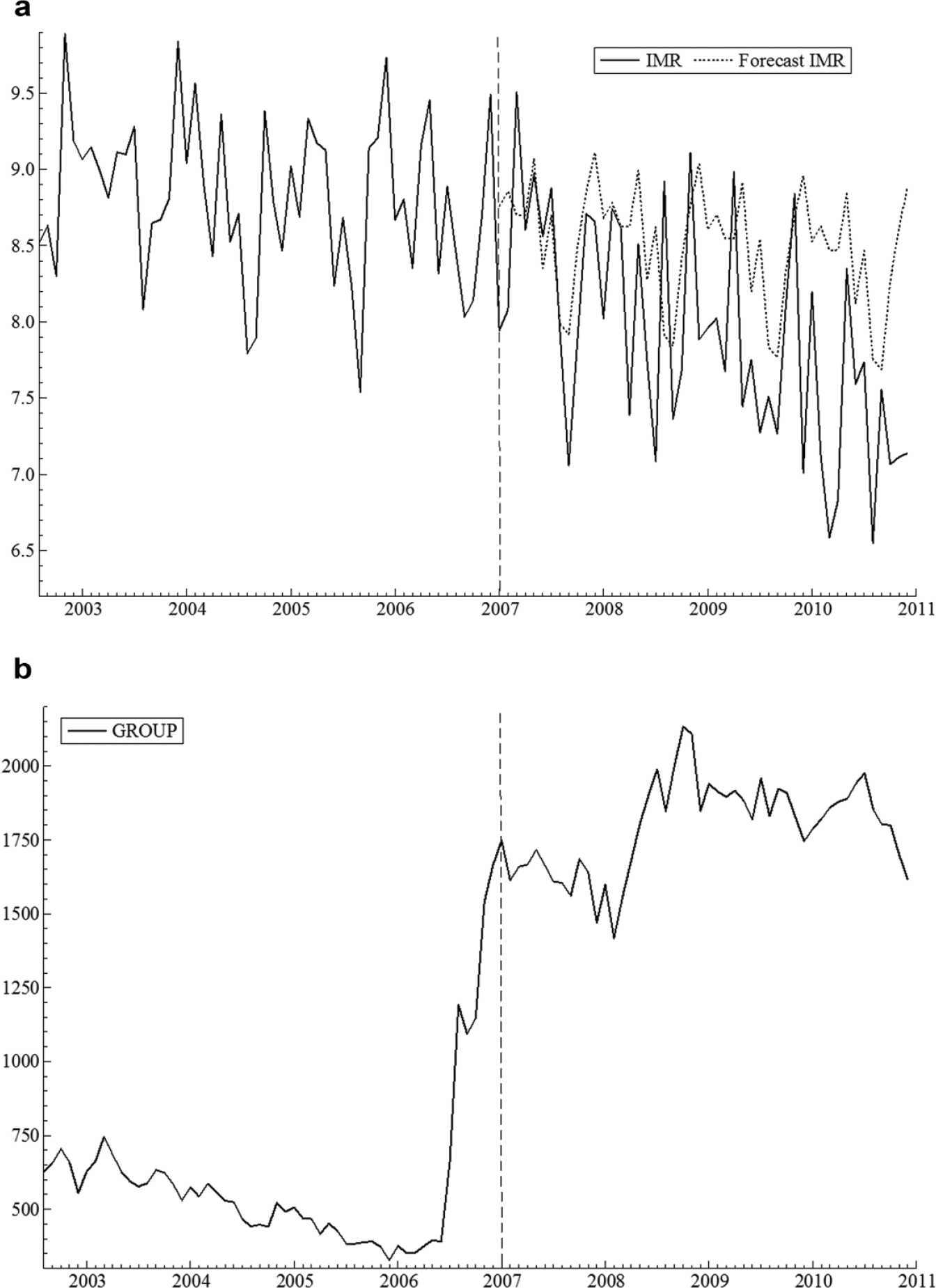
Plots of monthly IMR and size of the TM-Sidhi group (GROUP).

In the preintervention period, the IMR trend is relatively flat or very slightly negative with irregular variation and weak seasonal variation around the trend. Beginning in January 2007 (see vertical line in the plot), IMR displays a shift to a more rapidly declining trend that continues through the end of the sample period. During the intervention period, actual IMR declines more rapidly than predicted by its prior trend and faster than the IMR forecast.

Panel (b) of Figure 1 shows the plot of the GROUP series. As noted above, the GROUP plot approximates a step function, with an average of 591 participants for the 53-month baseline period compared with 1,792 for the 48-month intervention. In January 2007, the GROUP size for the first time in the sample period rose above the theoretically predicted critical threshold of 1,725, the √1% of the U.S. population.

Regression Results for IMR

To test the hypothesis of a decrease in the trend slope for IMR, we estimate the following broken-trend intervention model that incorporates a shift of linear trend beginning with the onset of the intervention (January 2007):

I M R_{t} = β_{0} + β_{1} t + (β_{2} - β_{1}) D T_{t} + \sum_{j} S_{j t} D_{j} + ε_{t} .

In Equation 1, β₀ is the regression intercept, t is a linear time trend (t = 1, 2, 3, . . ., N), and β₁ is the preintervention trend slope for IMR. The variable DT_t models the shift in trend due to the intervention with DT_t = (t − t_B)I_t, where t_B is the time of the hypothesized break in the linear trend function (December 2006) and I_t is a binary (0-1) indicator variable (step function) that takes the value zero for the preintervention period and 1.0 for the intervention period (t > t_B). The regression coefficient (β₂ − β₁) for DT_t gives the change in trend slope for IMR from the preintervention value (β₁) to the slope in the intervention period (β₂). The hypothesis of a negative shift in trend for IMR during the intervention implies (β₂ − β₁) < 0.

The summation term in Equation 1 is a deterministic seasonal component to control for the monthly seasonal variation in IMR. The seasonal component consists of 11 binary (0-1) seasonal dummy variables D_j (with monthly index j = 1, 2, . . ., 11 where January is denoted by j = 1; Granger & Newbold, 1986). The seasonal regression coefficient for each month is given by S_jt. Finally, ϵ_t is an independent and identically distributed, serially uncorrelated normal error with mean zero and variance σ².

Table 1 reports the ordinary least squares (OLS) regression results for Equation 1. The estimated preintervention trend for IMR is small but negative and significant. The shift in trend has negative sign, as hypothesized, and is highly significant, t(87) = −4.50, p = 2.1 × 10⁻⁵, effect size f = −0.482, a medium to large effect, indicating an acceleration of the preintervention declining trend during the intervention period 2007 to 2010. The absolute value of the effect size measure is the square root of Cohen’s f ² for a regression variable (or set of variables), with 0.59, 0.39, and 0.14 considered large, medium, and small effects, respectively (Cohen, 1988).⁶ Panel (a) of Figure 2 graphically compares the preintervention trend slope for IMR with that for 2007 to 2010 and Panel (b) displays the estimated trend shift parameter (−0.02292) with 95% confidence interval = [−0.0128, −0.0330]. Although we have a clear a priori directional hypothesis for the shift in trend, to be conservative, two-tailed tests are reported for the estimated trend shift (and all other parameters). For reasons discussed below, the results reported in Table 1 are based on t ratios that remain valid in the presence of heteroscedasticity and autocorrelation of the regression residuals (Newey & West, 1987). The trend shift remains highly significant using conventional OLS standard errors, t(87) = −3.32, p = .001, but the preintervention trend is not significantly different from zero, t(87) = −1.88, p = .064.

Table 1.

OLS Regression Analysis of Monthly U.S. IMR.

Parameter	Estimate	SE ^a	t ratio^b
β₀	9.360	0.235	39.87***
β₁	−6.875 × 10⁻³	2.129 × 10⁻³	−3.23**
β₂ − β₁	−2.292 × 10⁻²	5.091 × 10⁻³	−4.50***
S _1t	−0.233	0.288	−0.81
S _2t	−0.185	0.219	−0.84
S _3t	−0.192	0.265	−0.73
S _4t	−0.245	0.303	−0.81
S _5t	0.141	0.236	0.60
S _6t	−0.403	0.219	−1.84
S _7t	−0.297	0.261	−1.13
S _8t	−0.672	0.275	−2.44*
S _9t	−0.875	0.269	−3.25**
S _10t	−0.371	0.276	−1.34
S _11t	0.178	0.307	0.58
F statistic: F(13, 87) = 11.65***		Mean of IMR = 8.386
SE of regression = 0.501		SE of IMR = 0.774
Sum of squared residuals = 21.864		Log-likelihood = −66.033
R² = .635; Adjusted R² = .581		BIC = 1.947; AIC = 1.585
Diagnostics
Serial correlation test		Heteroscedasticity test
Lags 1-6: F(6, 81) = 3.370 (p = .005)		F(15, 85) = 1.234 (p = .263)
Lags 1-12: F(12, 75) = 1.948 (p = .042)		Test for ARCH
Normality test: χ²(2) = 1.260 (p = .533)		Lags 1-6: F(6, 89) = 6.803 (p = .570)
Robinson test^c: t(61) = −8.177 (p < .001)		Test of functional form
Perron unit root test: τ_α = −6.612 (p < .01)		F(2, 85) = 1.607 (p = .207)

Note. Sample is August 2002 to December 2010, N = 101. OLS = ordinary least squares; IMR = infant mortality rate; BIC = Bayesian information criterion; AIC = Akaike information criterion; ARCH = autoregressive conditional heteroscedasticity.

Newey–West SEs and t ratios (Newey & West, 1987).

df = 87.

Frequency domain test for nonstationarity (Robinson, 1995).

p < .05. **p < .01. ***p < .001.

Figure 2.

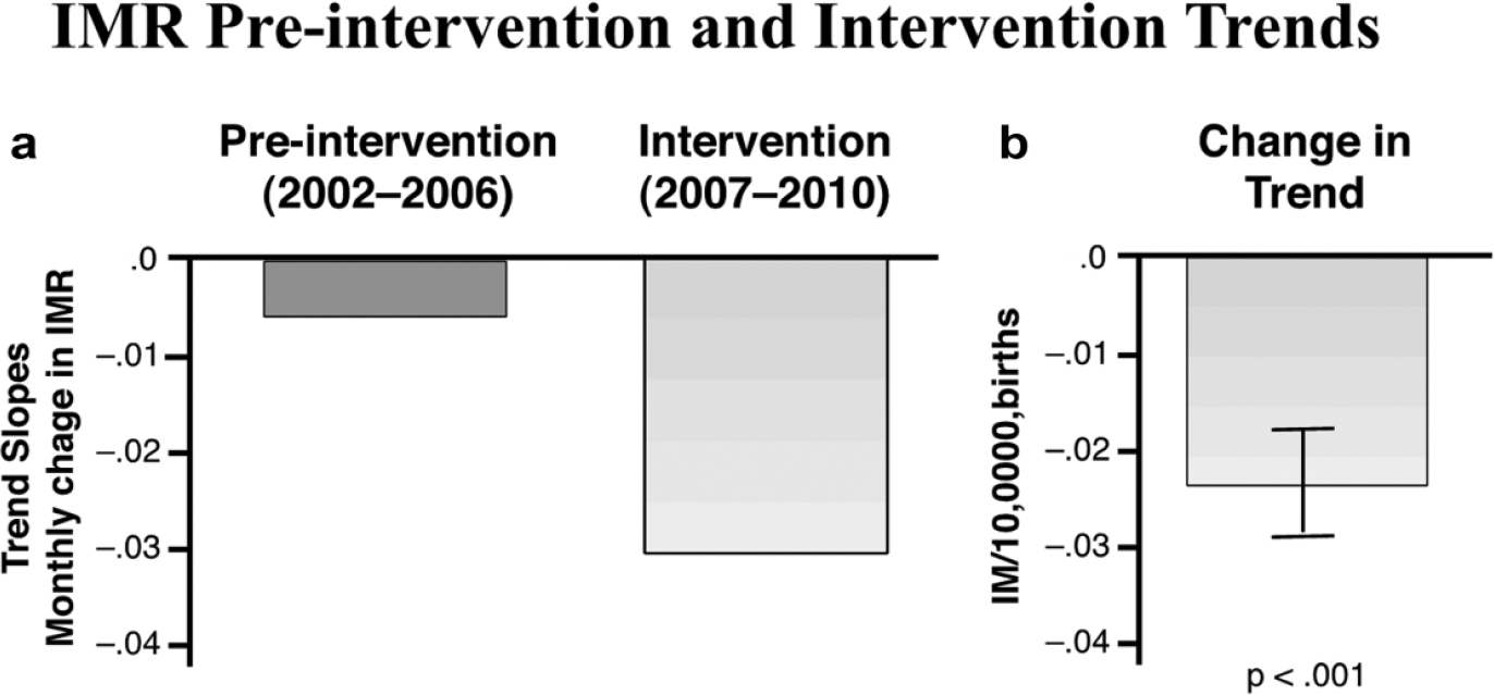
Comparison of mortality trends during the preintervention and intervention periods.

Relative to the preintervention trend, the estimated trend shift implies a total reduction of 1.100 in IMR during the 2007 through 2010 intervention period.⁷ This is a reduction of 12.47% (or 3.12% per year) compared with the mean preintervention monthly rate of 8.821 fatalities per 10,000 live births. The decline in IMR translates to a total of 992 averted infant deaths for 2007 to 2010, deaths projected to occur had the preintervention trend continued unchanged through 2007 to 2010.⁸ Thus, the estimated shift in trend for IMR during 2007 through 2010 has the predicted negative sign and is both statistically and practically significant. Statistical analysis (see Table 1) indicates that these results cannot be explained by seasonal variation, autocorrelation, or preexisting trends in IMR.

Regression Diagnostics for Analysis of IMR

Table 1 reports diagnostic tests for evaluating the adequacy of the estimated intervention model. The null hypothesis of serially uncorrelated (white noise) regression residuals at lags 1 to 6, and 1 to 12 is rejected by the Breusch–Godfrey Lagrange Multiplier (LM) test (Godfrey, 1978).⁹ Only one autocorrelation at lags 1 to 36 is statistically significant. The largest individual autocorrelations are at lag 1 (−0.208), which is just significant at the 5% level, and lags 4 (−0.196) and 16 (−0.224), which are nearly significant. Because of this modest serial correlation, Table 1 reports t ratios based on SEs that are valid (consistent) in the presence of serial correlation and heteroscedasticity of possibly unknown form (Newey & West, 1987).¹⁰

Although some mild autocorrelation is present, the autocorrelations are all small, and thus the residual series appears to be clearly stationary. A TS is said to be covariance stationary (or weakly stationary) if its mean, variance, and autocorrelations (or, equivalently, its autocovariances) are invariant with respect to a change in time origin (Enders, 2010). Empirical support for stationarity of the IMR residual series is provided by a frequency domain test based on the periodogram of regression residuals (Baum & Wiggins, 2000; Robinson, 1995). The Robinson test evaluates stationarity based on an empirical estimate of the order of integration of a TS, I(d), where d is the number of times the series must be differenced to induce stationarity. For example, in the case of a nonstationary random walk, the differencing parameter d = 1, and the series may be transformed to I(0), or stationarity, by first differencing. The Robinson test rejects the null hypothesis (p < .001) that the IMR residual series is nonstationary (see Table 1),¹¹ supporting the conclusion that IMR is broken-trend stationary, exhibiting stationary fluctuations around a broken trend.

Stationarity of the regression residuals is required for valid statistical inferences regarding the estimated regression parameters in the intervention model (Banerjee, Dolado, Galbraith, & Hendry, 1993; Enders, 2010; Granger & Newbold, 1986). Broken-trend stationarity for IMR implies that the OLS regression estimates in Table 1 have standard distributions and thus the observed significant change in trend is unlikely to be the result of “spurious regression” (Banerjee et al., 1993; Granger & Newbold, 1986). Spurious regressions can result when time trends are fitted to nonstationary variables that contain a random walk component (“stochastic trend”). A key signature of spurious regressions is highly autocorrelated, nonstationary regression residuals. The latter violate the distributional assumptions underlying statistical inference for TS regression.

Table 1 reports a formal test for broken-trend stationarity of a TS with a known (exogenous) structural break (Perron, 1989, 2006).¹² The Perron unit root test rejects the null hypothesis (p < .01) that the IMR TS is a nonstationary random walk with drift (Perron, 1989; Zivot & Andrews, 1992).¹³ The alternative hypothesis is that IMR is broken-trend stationary, displaying stationary fluctuations around a linear trend with a known, one-time break in the trend function in December 2006.¹⁴

The results of all other diagnostic tests for model adequacy are satisfactory. The null hypothesis of no autoregressive conditional heteroscedasticity (ARCH) for the regression residuals is not rejected by the LM test for ARCH (Engle, 1982). Likewise, White’s general test for heteroscedasticity (White, 1980) fails to reject the null hypothesis that the regression errors are homoscedastic or, if heteroscedasticity is present, it is unrelated to the regressors. The null hypothesis that the functional form of the regression model is correctly specified is not rejected by Ramsey’s (1969) Regression Error Specification Test (RESET). The omnibus Doornik–Hansen test for normality of the regression errors (Doornik & Hansen, 2008) fails to reject the null hypothesis that the errors are drawn from a normal distribution. No regression residuals exceed 3.5 standard errors, indicating the absence of extreme outliers. Thus, the diagnostic tests for model adequacy support statistical conclusion validity for the statistical inferences reported in Table 1.

Study 2: Results of Analysis of DFR

Plot of DFR

The plot of DFR in Figure 3 displays monthly seasonal fluctuations and a rising preintervention trend followed by a flattening of the trend slope in 2007 through 2010. During 2007 through 2010, the forecast of DFR (dotted line) based on preintervention data continues DFR’s preintervention upward trend, rising substantially above observed DFR (see Note 18).

Figure 3.

Plot of monthly DFR.

Regression Results for DFR

We estimate the following broken-trend intervention model to test the hypothesis of a shift to a reduced trend slope for DFR during the intervention period:

\begin{array}{l} D F R_{t} = β_{0} + β_{1} t + (β_{2} - β_{1}) D T_{t} + β_{3} D F R_{t - 1} + \\ \sum_{j} S_{j t} D_{j} + ε_{t} . \end{array}

where lag 1 of DFR_t is included (with regression coefficient β₃) to model its first-order autoregressive dynamics. All other terms are defined as in Equation 1.

The OLS regression estimates of the model coefficients for Equation 2 are reported in Table 2. The DFR preintervention trend is positive and significant. The change in trend has negative sign and is highly significant, consistent with theoretical prediction.

Table 2.

OLS Regression Analysis of Monthly U.S. DFR.

Parameter	Estimate	SE ^a	t ratio^b
β₀	3.484	0.606	5.76***
β₁	2.998 × 10⁻²	6.266 × 10⁻³	4.78***
β₂ − β₁	−2.897 × 10⁻²	6.968 × 10⁻³	−4.16***
β₃	0.498	9.560 × 10⁻²	5.21***
S _1t	0.276	0.146	1.89
S _2t	−0.417	0.160	−2.61**
S _3t	0.507	0.146	3.47***
S _4t	−0.336	0.170	−1.97
S _5t	0.305	0.150	2.03*
S _6t	−0.433	0.165	−2.63**
S _7t	0.189	0.147	1.29
S _8t	−0.223	0.154	−1.45
S _9t	−0.529	0.145	−3.64***
S _10t	−0.091	0.139	−0.65
S _11t	−0.422	0.141	−2.99**
F statistic: F(14, 86) = 102.30**		Mean of DFR = 9.856
SE of regression = 0.296		SE of DFR = 1.152
Sum of squared residuals = 7.523		Log-likelihood = −12.159
R² = .943; Adjusted R² = .934		BIC = 0.926; AIC = 0.538
Diagnostics
Serial correlation test		Heteroscedasticity test
Lags 1-6: F(6, 80) = 0.918 (p = .487)		F(19, 81) = 1.359 (p = .172)
Lags 1-12: F(12, 74) = 0.823 (p = .627)		Test for ARCH
Normality test: χ²(2) = 0.951 (p = .622)		Lags 1-6: F(6, 89) = 0.883 (p = .511)
Robinson test^c: t(61) = −6.175 (p < .001)		Test of functional form
Perron unit root test: τ_α = −6.477 (p < .01)		F(2, 84) = 1.990 (p = .143)

Note. Sample is August 2002 to December 2010, N = 101. OLS = ordinary least squares; DFR = drug-related fatality rate; BIC = Bayesian information criterion; AIC = Akaike information criterion; ARCH = autoregressive conditional heteroscedasticity.

OLS SEs and t ratios.

df = 86.

Frequency domain test for nonstationarity (Robinson, 1995).

p < .05. **p < .01. ***p < .001.

In Table 2, the regression estimate of β₂ − β₁, the change in trend, gives the initial intervention impact. The significant first-order autoregressive dynamics of DFR around the trend implies a gradual adjustment of the preintervention trend to its equilibrium, or long-run, value after onset of the intervention. If (1 − β₃) ≠ 0, the total change in trend is given by κ = (β₂ − β₁) / (1 − β₃). A formal test rejects the hypothesis (1 − β₃) = 0 (p < .01) in favor of the alternative that (|β₃| < 1), indicating that the estimated model is dynamically stable and thus that the trend will converge to its equilibrium value κ in the long run (Banerjee, Dolado, & Mestre, 1998; Doornik & Hendry, 2013; Enders, 2010). For the DFR analysis κ = −0.0578, t(86) = −7.12, p = 3.1 × 10⁻¹⁰, effect size f = −0.449, a medium to large effect, and 95% confidence interval = [−0.0417, −0.0739], where κ is the coefficient on DT_t in the long-run equation for DFR (Hendry, 1995).¹⁵ In this context, “long run” denotes the mathematically expected equilibrium value and does not necessarily imply a long period of time (Hendry, 1995). The estimated cumulative lag weights for Equation 2 indicate that 50.2%, 75.25%, 87.6%, and 93.8% of the adjustment in trend after the onset of the intervention is completed within 1, 2, 3, and 4 months, respectively. Panel (a) of Figure 4 compares the equilibrium trend slopes for the preintervention and 2007 through 2010 periods and Panel (b) shows the estimated trend shift with 95% confidence interval.¹⁶

Figure 4.

Comparison of DFR trends during the preintervention and intervention periods.

Relative to the preintervention trend, the equilibrium trend shift for 2007 to 2010 implies a total cumulative decline in DFR of 2.7723 monthly fatalities per million population during the intervention period.¹⁷ This is a reduction of 30.42% (or 7.61% annually) compared with the mean preintervention monthly rate of 9.112 fatalities per million people. The decline in DFR translates to a projected total of 26,425 averted drug-related fatalities for 2007 to 2010.¹⁸ Thus, the estimated shift in trend for DFR is negative, as predicted, and both practically and statistically significant. The statistical findings reported in Table 2 suggest that these results cannot be explained by autocorrelation, seasonal variation, or preexisting trends in DFR.

Regression Diagnostics for DFR

All diagnostic tests reported in Table 2 for adequacy of the estimated intervention model are satisfactory. That no regression residuals exceed 3.5 standard errors indicates the absence of extreme outliers. The LM tests for autocorrelation of residuals at lags 1 to 6 and lags 1 to 12 are not significant, and no autocorrelations at lags 1 to 36 are individually significant, indicating that the regression residuals appear to be serially uncorrelated, stationary white noise. The frequency domain test (Baum & Wiggins, 2000; Robinson, 1995) rejects the null hypothesis (p < .001) that the residual series is nonstationary (see Table 2).¹⁹ The latter test, plus the absence of significant residual autocorrelation, lend further support to the conclusion of the Perron test (see Table 2) that DFR is likely broken-trend stationary.²⁰ Thus, the diagnostic tests for adequacy of the broken-trend regression model support statistical conclusion validity for the statistical inferences reported in Table 2.

Discussion

The results of the two studies indicate that, as hypothesized, there was a significant and substantial reduction of the trends of IMR and DFR during the intervention period 2007 through 2010, beginning in January 2007 with the onset of the intervention. The null hypothesis of no effect of the intervention on mortality trends was strongly rejected for both mortality rate series. Diagnostic tests for the broken-trend intervention analysis indicate the appropriateness of the statistical assumptions underlying the analyses. These results are thus consistent with the conclusion that the intervention may have contributed to the observed trend shifts for both mortality rates.

The use of an intervention at the national level in a prospective quasi-experimental design is inherently stronger as a design than an ex post analysis of archival data on the relationship of interdependent factors using variants of multiple regression analysis (Glass, 1997). Nevertheless, it is necessary to consider possible threats to internal validity, namely, alternative possible causes of the reduction of the stress-related mortality variables investigated in these studies.

A major societal impact that occurred during the intervention period was the economic recession of 2008-2009 associated with the subprime mortgage crisis. However, the onset and duration of this recession (December 2007, with peak unemployment in October 2009) does not precisely track the intervention period. More importantly, the economic stresses associated with the recession (e.g., unemployment) would be predicted, if anything, to increase rather than decrease the stress-related health indicators examined in these studies.

One specific factor to consider in the case of drug-related deaths is that one might speculate that increased public and professional awareness of the hazards of opioid analgesics in recent years might have contributed to a reduction in their prescription during the intervention period. As outlined in the introduction, increased used of opioid drugs is considered to contribute substantially to the rise of DD. However, data indicate that opioid sales increased throughout the baseline and intervention period of this research, reaching their peak in 2011 (Volkow, 2014). Thus, the opioids were becoming more available rather than less available through the intervention period.

Because of the national scope of measurement of these studies, and the specificity of the intervention period and associated changes in mortality rates, a viable alternative explanation will require almost simultaneous implementation of a treatment or medical technology or program that would influence both the variables of these studies and disproportionately affect two different subpopulations of the United States (higher prevalence for African American women in the case of IM and for middle-age Whites in the case of DD). We are unable to think of any such plausible alternative explanation that would satisfy these two requirements. In the absence of plausible alternative explanations, the significant intervention impacts on both mortality variables found in this article suggest the possibility of some underlying connection between individuals who are not apparently behaviorally connected. As outlined in the introduction to this article, such a connection independent of behavioral interaction is described as the collective consciousness of society. More specifically, the Vedic tradition of India identifies collective consciousness as having its basis in an underlying level of pure consciousness, which is predicted to be influenced by the intervention examined here, group practice of the advanced TM-Sidhi program.

An alternative hypothesis affecting generalizability of the results is whether there is selection bias in the use of members in the intervention group who were already experts in the Transcendental Meditation and TM-Sidhi program and may therefore be a special group in terms of consciousness training. From a theoretical perspective, it is only necessary that the members of the intervention group be trained in the advanced TM-Sidhi program to stimulate the hypothesized field of pure consciousness. It is understood that, as a practical necessity, the individuals who participated in this project would be those with some prior expertise/training to volunteer their time. But, in principle, for this effect to be created, any group with basic stability, such as groups of students or the military, could be employed once trained in the TM-Sidhi program. In some countries, such groups are being created and future research will be necessary to confirm their effects.

The result of these studies, if further replicated, provide government leaders with a potential means to relieve stress on a large scale in society that is independent of structural social change and benefits public health. Although social stress as a mediating variable was not directly measured, the consistency of the present results with those reported previously for reduced homicide and violent crime (Dillbeck & Cavanaugh, 2016) lends support to a hypothesis of such a mediating influence. In light of these results, it is suggested that when TM-Sidhi groups are established with government support (most easily, with existing groups, such as military personnel), the potential impact of such TM-Sidhi groups be evaluated on stress-related public health parameters.

Footnotes

Acknowledgements

The authors appreciate the cooperation of the Invincible America Assembly Office of Maharishi University of Management for providing group meditation data used in this study. The second author acknowledges access to the use of a university laptop and software for this research.

Authors’ Note

Raw data may be obtained from the first author.

Declaration of Conflicting Interests

The authors declared no potential conflicts of interest with respect to the research, authorship, and/or publication of this article: The authors have no financial relationship with the foundation that teaches Transcendental Meditation in the United States (Maharishi Foundation USA). The first author is a Trustee and research professor and the second author is a retired faculty member of the university sponsoring the project evaluated in this research, but both currently receive no financial compensation from the university for their research or other activities, which are donated as contributed services.

Funding

The authors received no financial support for the research and/or authorship of this article.

Notes

Author Biographies

Michael C. Dillbeck, PhD, is a research scientist at the Institute of Science, Technology and Public Policy and research professor and Trustee at Maharishi University of Management. His research spans the physiological, psychological, and sociological effects on the Transcendental Meditation and TM-Sidhi programs.

Kenneth L. Cavanaugh, PhD, is a senior research scientist at the Institute of Science, Technology and Public Policy and a professor of Applied Statistics, Emeritus at Maharishi University of Management. His currrent principal research interest is empirical study of the hypothesized effects of the group practice of the TM-Sidhi program on societal quality of life.

References

Alexander

C. N.

Davies

J. L.

Dixon

Dillbeck

M. C.

Druker

Oetzel

R. M.

. . . Orme-Johnson

D. W.

(1990). Growth of higher states of consciousness: Maharishi’s Vedic psychology of human development. In Alexander

C. N.

Langer

E. J.

(Eds.), Higher stages of human development: Perspectives on adult growth (pp. 286-340). New York, NY: Oxford University Press.

Assimakis

P. D.

Dillbeck

M. C.

(1995). Time series analysis of improved quality of life in Canada: Social change, collective consciousness, and the TM-Sidhi program. Psychological Reports, 76, 1171-1193. doi:10.2466/pr0.1995.76.3c.1171

Banerjee

Dolado

J. J.

Galbraith

J. W.

Hendry

D. F.

(1993). Co-integration, error correction and the econometric analysis of non-stationary data. Oxford, UK: Oxford University Press.

Banerjee

Dolado

J. J.

Mestre

(1998). Error-correction mechanism tests for cointegration in a single equation framework. Journal of Time Series Analysis, 19, 267-283.

Bårdsen

(1989). The estimation of long-run coefficients from error-correction models. Oxford Bulletin of Economics and Statistics, 51, 345-350. doi:10.1111/j.1468-0084.1989.mp51003008.x

Baum

C. F.

Wiggins

(2000). Tests for long memory in a time series. Stata Technical Bulletin, 57, 39-44.

Box

G. E. P.

Jenkins

G. M.

(1976). Time series analysis: Forecasting and control. San Francisco, CA: Holden-Day.

Case

Deaton

(2015). Rising morbidity and mortality in midlife among white non-Hispanic Americans in the 21st century. Proceedings of the National Academy of Sciences of the United States of America, 112(49), 15078-15083. doi:10.1073/pnas.1518393112

Cavanaugh

K. L.

Dillbeck

M. C.

(2017). The contribution of proposed field effects of consciousness to the prevention of US accidental fatalities: Theory and empirical tests. Journal of Consciousness Studies, 24, 53-86.

10.

Centers for Disease Control and Prevention, National Center for Health Statistics. (2012). Underlying cause of death, 1999-2010 on CDC WONDER online database, released 2012. Retrieved from http://wonder.cdc.gov/ucd-icd10.html

11.

Centers for Disease Control and Prevention, National Center for Health Statistics. (2015a). Underlying cause of death 1999-2013 on CDC WONDER online database, released 2015. Retrieved from http://wonder.cdc.gov/ucd-icd10.html

12.

Centers for Disease Control and Prevention, National Center for Health Statistics. (2015b). Natality public use data 2003-2006, 2007-2013 on CDC WONDER online database, released 2012. Retrieved from http://wonder.cdc.gov/natality-v2006.html and http://wonder.cdc.gov/natality-current.html

13.

Chelimsky

Shadish

W. R.

Orwin

R. G.

(1997). Twenty-one years and counting: The interrupted time series comes of age. In Chelimsky

Shadish

(Eds.), Evaluation for the 21st century (pp. 443-465). London, England: Sage.

14.

Cohen

(1988). Statistical power analysis for the behavioral sciences (2nd ed.). Hillsdale, NJ: Lawrence Erlbaum.

15.

Cook

T. D.

Campbell

D. T.

(1979). Quasi-experimentation: Design and analysis issues for field settings. Boston, MA: Houghton Mifflin.

16.

Darlington

R. B.

(1990). Regression and linear models. New York, NY: McGraw-Hill.

17.

Davies

J. L.

Alexander

C. N.

(2005). Alleviating political violence through reducing collective tension: Impact assessment analyses of the Lebanon war. Journal of Social Behavior and Personality, 17, 285-338.

18.

Dickey

Fuller

W. A.

(1979). Distribution of the estimates for autoregressive time series with a unit root. Journal of the American Statistical Association, 74, 427-431.

19.

Dillbeck

M. C.

(1990). Test of a field hypothesis of consciousness and social change: Time series analysis of participation in the TM-Sidhi program and reduction of violent death in the U.S. Social Indicators Research, 22, 399-418. doi:10.1007/BF00303834

20.

Dillbeck

M. C.

Alexander

C. N.

(1989). Higher states of consciousness: Maharishi Mahesh Yogi’s Vedic psychology of human development. The Journal of Mind and Behavior, 10, 307-334.

21.

Dillbeck

M. C.

Banus

C. B.

Polanzi

Landrith

G. S.

III . (1988). Test of a field model of consciousness and social change: Transcendental Meditation and TM-Sidhi program and decreased urban crime. The Journal of Mind and Behavior, 9, 457-486.

22.

Dillbeck

M. C.

Bronson

E. C.

(1981). Short-term longitudinal effects of the Transcendental Meditation technique on EEG power and coherence. International Journal of Neuroscience, 14, 147-151. doi:10.3109/00207458108985827

23.

Dillbeck

M. C.

Cavanaugh

K. L.

(2016). Societal violence and collective consciousness: Reduction of U.S. homicide and urban violent crime rates. SAGE Open, 6(2), 1-16. doi:10.1177/2158244016637891

24.

Dillbeck

M. C.

Cavanaugh

K. L.

Glenn

Orme-Johnson

D. W.

Mittlefehldt

(1987). Effects of Transcendental Meditation and the TM-Sidhi program on quality of life indicators: Consciousness as a field. The Journal of Mind and Behavior, 8, 67-104.

25.

Dillbeck

M. C.

Orme-Johnson

D. W.

(1987). Physiological differences between Transcendental Meditation and rest. American Psychologist, 42, 879-881. doi:10.1037/0003-066X.42.9.879

26.

Dillbeck

M. C.

Rainforth

M. V.

(1996). Impact assessment analysis of behavioral quality of life indices: Effects of group practice of the Transcendental Meditation and TM-Sidhi program. Proceedings of the American Statistical Association, Social Statistics Section, 38-43.

27.

Dole

Savitz

D. A.

Hertz-Picciotto

Siega-Riz

A. M.

McMahon

M. J.

Buekens

(2003). Maternal stress and preterm birth. American Journal of Epidemiology, 157, 14-24. doi:10.1093/aje/kwf176

28.

Doornik

J. A.

Hansen

(2008). An omnibus test for univariate and multivariate normality. Oxford Bulletin of Economics and Statistics, 70, 927-939. doi:10.1111/j.1468-0084.2008.00537.x

29.

Doornik

J. A.

Hendry

D. F.

(2013). Empirical econometric modelling–PcGive 14: Volume 1. London, England: Timberlake Consultants Press.

30.

Enders

(2010). Applied econometric time series (3rd ed.). Hoboken, NJ: John Wiley.

31.

Engle

R. F.

(1982). Autoregressive conditional heteroscedasticity with estimates of the variance of United Kingdom inflation. Econometrica, 50, 987-1007.

32.

Gennaro

Hennessy

M. D.

(2003). Psychological and physiological stress: Impact on preterm birth. Journal of Obstetric, Gynecologic & Neonatal Nursing, 32, 668-675. doi:10.1177/0884217503257484

33.

Glass

G. V.

(1997). Interrupted time series quasi-experiments. In Jaeger

R. M.

(Ed.), Complementary methods for research in education (2nd ed., pp. 589-608). Washington, DC: American Educational Research Association.

34.

Godfrey

L. G.

(1978). Testing for higher order serial correlation in regression equations when the regressors include lagged dependent variables. Econometrica, 46, 1303-1313. doi:10.2307/1913830

35.

Granger

C. W. J.

Newbold

(1986). Forecasting economic time series (2nd ed.). Orlando, FL: Academic Press.

36.

Greene

W. H.

(2011). Econometric analysis (7th ed.). Upper Saddle River, NJ: Prentice Hall.

37.

Hagelin

J. S.

(1987). Is consciousness the unified field? A field theorist’s perspective. Modern Science and Vedic Science, 1, 28-87.

38.

Hagelin

J. S.

Rainforth

M. V.

Orme-Johnson

D. W.

Cavanaugh

K. L.

Alexander

C. N.

Shatkin

S. F.

. . . Ross

(1999). Effects of group practice of the Transcendental Meditation program on preventing violent crime in Washington, DC: Results of the National Demonstration Project, June-July 1993. Social Indicators Research, 47, 153-201. doi:10.1023/A:1006978911496

39.

Harmon

(2010, April 6). Prescription drug deaths increase dramatically. Scientific American. Retrieved from http://www.scientificamerican.com/article/prescription-drug-deaths/

40.

Harvey

(1990). The econometric analysis of time series (2nd ed.). Cambridge, MA: MIT Press.

41.

Hatchard

G. D.

Deans

A. J.

Cavanaugh

K. L.

Orme-Johnson

D. W.

(1996). The Maharishi effect: A model for social improvement. Time series analysis of a phase transition to reduced crime in Merseyside metropolitan area. Psychology, Crime & Law, 2, 165-174. doi:10.1080/10683169608409775

42.

Hendry

D. F.

(1995). Dynamic econometrics. Oxford, UK: Oxford University Press.

43.

Inder

(1993). Estimating long-run relationships in economics: A comparison of different approaches. Journal of Econometrics, 57, 53-68. doi:10.1016/0304-4076(93)90058-D

44.

Jevning

Wilson

A. F.

Davidson

J. M.

(1978). Adrenocortical activity during meditation. Hormones and Behavior, 10, 54-60.

45.

Jones

C. M.

Mack

K. A.

Paulozzi

L. J.

(2013). Pharmaceutical overdose deaths, United States, 2010. Journal of the American Medical Association, 309, 657-659.

46.

Kiviet

J. F.

(1986). On the rigour of some misspecification tests for modelling dynamic relationships. Review of Economic Studies, 53, 241-261. doi:10.2307/2297649

47.

Latendresse

(2009). The interaction between chronic stress and pregnancy: Preterm birth from a biobehavioral perspective. Journal of Midwifery & Women’s Health, 54, 8-17. doi:10.1016./j.jmwh.2008.08.001

48.

Linsky

A. S.

Bachman

Straus

M. A.

(1995). Stress, culture, & aggression. New Haven, CT: Yale University Press.

49.

Linsky

A. S.

Straus

M. A.

(1986). Social stress in the United States. Dover, MA: Auburn House Publishing.

50.

MacDorman

M. F.

Mathews

T. J.

(2008). Recent trends in infant mortality in the United States (NCHS Data Brief, No. 9). Hyattsville, MD: National Center for Health Statistics.

51.

MacDorman

M. F.

Mathews

T. J.

(2011). Understanding racial and ethnic disparities in U.S. infant mortality rates (NCHS Data Brief, No. 74). Hyattsville, MD: National Center for Health Statistics.

52.

MacDorman

M. F.

Mathews

T. J.

Mohangoo

A. D.

Zeitlin

(2014, September 4). International comparisons of infant mortality and related factors: United States and Europe, 2010 (National Vital Statistics Reports, Vol. 63, Number 5). Hyattsville, MD: National Center for Health Statistics.

53.

MacLean

C. R. K.

Walton

K. G.

Wenneberg

S. R.

Levitsky

D. K.

Mandarino

J. P.

Waziri

. . . Schneider

R. H.

(1997). Effects of the Transcendental Meditation program on adaptive mechanisms: Changes in hormone levels and responses to stress after 4 months of practice. Psychoneuroendocrinology, 22, 277-295.

54.

Maharishi Mahesh Yogi. (1969). Maharishi Mahesh Yogi on the Bhagavad-Gita: A new translation and commentary, chapters 1 to 6. Baltimore, MD: Penguin.

55.

Maharishi Mahesh Yogi. (1977). Creating an ideal society. Rheinweiler, Germany: Maharishi European Research University Press.

56.

Maharishi Mahesh Yogi. (1986). Life supported by natural law. Washington, DC: Age of Enlightenment Press.

57.

Mathews

T. J.

MacDorman

M. F.

Thoma

M. E.

(2015, August 6). Infant mortality statistics from the 2013 period linked birth/infant death data set (National Vital Statistics Reports, Vol. 64, Number 9). Hyattsville, MD: National Center for Health Statistics.

58.

Newey

W. K.

West

(1987). A simple positive semi-definite, heteroscedasticity and autocorrelation consistent covariance matrix. Econometrica, 55, 703-708.

59.

Orme-Johnson

D. W.

Alexander

C. N.

Davies

J. L.

(1990). The effects of the Maharishi Technology of the Unified Field: Reply to a methodological critique. Journal of Conflict Resolution, 34, 756-768. doi:10.1177/0022002790034004009

60.

Orme-Johnson

D. W.

Alexander

C. N.

Davies

J. L.

Chandler

H. M.

Larimore

W. E.

(1988). International peace project in the Middle East: The effects of the Maharishi Technology of the Unified Field. Journal of Conflict Resolution, 32, 776-812. doi:10.1177/0022002788032004009

61.

Orme-Johnson

D. W.

Oates

R. M.

(2009). A field-theoretic view of consciousness: Reply to critics. Journal of Scientific Exploration, 23, 139-166.

62.

Paulozzi

L. J.

Budnitz

D. S.

(2006). Increasing deaths from opioid analgesics in the United States. Pharmacoepidemiology & Drug Safety, 15, 618-625. doi:10.1002/pds.1276

63.

Perron

(1989). The great crash, the oil price shock, and the unit root hypothesis. Econometrica, 57, 1361-1401. doi:10.2307/1913712

64.

Perron

(2006). Dealing with structural breaks. In Mills

T. C.

Patterson

(Eds.), Palgrave handbook of econometrics, Vol. 1: Econometric theory (pp. 278-352). Basingstoke, UK: Palgrave Macmillan.

65.

Radhakrishnan

(1953). Principal Upanishads. New York, NY: Harper.

66.

Ramsey

J. B.

(1969). Tests for specification errors in classical linear least squares regression analysis. Journal of the Royal Statistical Society: Series B—Methodological, 31, 350-371.

67.

Rappoport

Reichlin

(1989). Segmented trends and non-stationary time series. Economic Journal, 99, 168-177.

68.

Robinson

P. M.

(1995). Log-periodogram regression of time series with long range dependence. Annals of Statistics, 23, 1048-1072.

69.

Roth

(2002). Maharishi Mahesh Yogi’s Transcendental Meditation. Washington, DC: Primus.

70.

Said

S. E.

Dickey

(1984). Testing for unit roots in autoregressive moving-average models with unknown order. Biometrika, 71, 599-607. doi:10.1093/biomet/71.3.599

71.

Schneider

R. H.

Carr

(2014). Transcendental Meditation in the prevention and treatment of cardiovascular disease and pathophysiological mechanisms: An evidence-based review. Advances in Integrative Medicine, 1, 107-112. doi:10.1016/j.aimed.2014.08.003

72.

Shadish

W. R.

Cook

T. D.

Campbell

D. T.

(2002). Experimental and quasi-experimental designs for generalized causal inference. Boston, MA: Houghton Mifflin.

73.

Sinha

(2008). Chronic stress, drug use, and vulnerability to addiction. Annals of the New York Academy of Sciences, 1141, 105-130. doi:10.1196/annals.141.030

74.

StataCorp. (2015). Stata Statistical Software: Release 14. College Station, TX: Author.

75.

Travis

Haaga

D. A. F.

Hagelin

Tanner

Arenander

Nidich

. . . Schneider

R. H.

(2010). A self-referential default brain state: Patterns of coherence, power, and eLORETA sources during eye-closed rest and Transcendental Meditation practice. Cognitive Processing, 11, 21-30. doi:10.1007/s10339-009-0343-2

76.

Travis

Haaga

D. A. F.

Hagelin

Tanner

Nidich

Gaylord-King

. . . Schneider

R. H.

(2009). Effects of Transcendental Meditation practice on brain functioning and stress reactivity in college students. International Journal of Psychophysiology, 71, 170-176. doi:10.1016/j.ijpsycho.2008.09.007

77.

Volkow

N. D.

(2014, May 4). Testimony to Congress—America’s addiction to opioids: Heroin and prescription drug abuse. National Institute on Drug Abuse of the National Institutes of Health. Retrieved from http://www.drugabuse.gov/about-nida/legislative-activities/testimony-to-congress/2015/americas-addiction-to-opioids-heroin-prescription-drug-abuse

78.

Walton

K. G.

Fields

J. Z.

Levitsky

D. K.

Harris

D. A.

Pugh

N. D.

Schneider

R. H.

(2004). Lowering cortisol and CVD risk in postmenopausal women: A pilot study using the Transcendental Meditation program. Annals of the New York Academy of Sciences, 1032, 211-215.

79.

White

(1980). A heteroskedastic-consistent covariance matrix estimator and a direct test for heteroskedasticity. Econometrica, 48, 817-838. doi:10.2307/1912934

80.

Zivot

Andrews

(1992). Further evidence on the great crash, the oil price shock, and the unit root hypothesis. Journal of Business & Economic Statistics, 10, 251-270. doi:10.1080/07350015.1992.10509904

Group Practice of the Transcendental Meditation® and TM-Sidhi® Program and Reductions in Infant Mortality and Drug-Related Death

Abstract

Keywords

General Method

Intervention

Dependent Variables

Data Analysis

Study 1: Results of Analysis of Monthly IMR

Plot of Monthly IMR

Regression Results for IMR

Regression Diagnostics for Analysis of IMR

Study 2: Results of Analysis of DFR

Plot of DFR

Regression Results for DFR

Regression Diagnostics for DFR

Discussion

Footnotes

Acknowledgements

Authors’ Note

Declaration of Conflicting Interests

Funding

Notes

Author Biographies

References