Refrigeration and the Reduction of the Takeoff Rate of Bushmeat

Abstract

Rising incomes in the developing world has led to increased consumption of bushmeat as a luxury good with a mounting risk of species extirpation. In a two-period model with stochastic supply, this article shows that the simple expedient of introducing refrigeration to the bushmeat markets can lead to the reduction of harvest rates. In the absence of refrigeration, all bushmeat brought to the market must be sold immediately, putting downward pressure on price and sending the incorrect signal to hunters that everything they kill can and will be sold. With refrigeration, it is possible to carry over inventory from one period to the next, which in turn limits harvests. Although harvest rates fall unequivocally, there may be no incentive for market participants to introduce refrigeration. This last result is explained through the use of the economists’ notion of economic welfare as measured by consumer and producer surplus. Achieving the socially desirable goal of lower harvest rates may require third-party intervention in the market.

Introduction

The model presented in this article demonstrates that the simple expedient of adopting a technical innovation (TI) such as refrigeration may reduce the consumption pressure on a sustainable wildlife resource. ¹ This occurs because the ability to carry over inventory from one period to the next permits retailers to gain some control over hunters’ harvest rates in the rain forest. In spite of this positive impact on harvest rates, refrigeration is slow to be adopted in developing economies, resulting in the possible extirpation of certain species. ² Using producer and consumer surplus, the model presented here can account for the slow pace of adoption. The observed hysteresis is the direct consequence of the ambiguous effect on consumer and producer surplus resulting from the adoption of a technological improvement in the form of refrigeration. For certain parameter values in the model, the sum of consumer surplus and producer surplus (understood as economic welfare) may actually decrease with the introduction of technologic improvement. ³ In that instance, there would be no private sector incentive for the adoption of the TI, even though adoption reduces the harvest rate of the endangered species.

The importance of TIs for economic growth and development has been in the forefront of the economics literature for many decades. The particular TI considered in this article is a well-known innovation from about a century ago and which is still not universal in today’s world. More than 100 years ago, electric refrigeration was introduced to the modern world as a tool for food storage and preservation (Yenne & Gross (1993)). Prior to electro-mechanical refrigeration, the principal methods for food storage were salting and smoking of commodities such as fish, chicken, beef, and other meat products. ⁴ Refrigeration resulted in added shelf life for all types of fresh produce (Woodford, 1997). Overall, the technical improvement of refrigeration resulted in cheaper and more efficient systems of inventory holding and supply chain management by increasing the shelf life for perishables.

Producers gain from more revenue and greater profit that result from their better use of resources achieved by the adoption of any TI. Besides the lower production costs, refrigeration also benefits consumers with better quality products having longer shelf life, improved taste, and more diversified uses of the upgraded products. As a result, we can expect a significant impact of TI on society. ⁵ Despite the benefits that its adoption may confer, TI is often overlooked. This article addresses the question of why available technical improvements such as refrigeration are not adopted in less developed countries, and the consequences for bushmeat in particular.

The motivating instance is the bushmeat trade in Equatorial Guinea. ⁶ Prior to 2007, there was very limited refrigeration in the bushmeat market in the capitol city of Malabo. We explore the role that the TI of refrigeration can play in coordinating the activities of producers and consumers with the consequence that markets clear without sellers resorting to drastic price reductions that would otherwise be needed to dispose of perishable goods (see, for example, Herbon, Spiegel, & Templeman, 2012).

Background for the Bushmeat Trade

In Equatorial Guinea, the most common way bushmeat is sold is through market women, known as mamás, who resell the animals directly to consumers in Malabo’s central market. Hunters in the rain forest utilize the convenience of the scheduled presence of the mamás to get their harvest into the hands of consumers (Cronin et al., 2015). The mamás are locally known as boyonselars (“buy-and-sellers” in the country’s pidgin). Three different practices are employed to get the meat to market. As the market has evolved, the most common method entails the mamás going by taxi to Luba, Riaba, and Moka weekly, stopping in every hunting camp, roadside station, and some villages to buy bushmeat. Once the mamás reach Luba, Riaba, or Moka, they meet with hunters and buy all the bushmeat available. The second method is when hunters give a taxi driver a labeled sack with the bushmeat in it, as well as a letter regarding its distribution. This letter, addressed to one of the mamás, explains in detail the contents of the sack, including the expected selling price of each animal. Mamás pay the driver Fcfa 1,000 to 2,000 (US$2-US$4), depending on how many animals the sack contains. Those hunters using taxis to deliver their product go themselves to Malabo to be paid by the mamás two or three times per month, receiving around Fcfa 100,000 (US$200) each time. Occasionally, a third method is employed, whereby the wives of the hunters (all the hunters are men) take bushmeat and agricultural produce directly to Malabo by taxi.

The carcass may be several days old ⁷ by the time it is in the hands of the mamá (note the flies swarming the carcasses on display at the seller’s stand of the typical mamá, Figure 1), and she, therefore, has much reduced bargaining power in her negotiations with consumers (Morra, Hearn, & Buck, 2009). The consequence is that nearly every carcass that comes to market is sold within a day of the time it arrives, ⁸ and there is no ability or incentive to manage the takeoff rate of the hunters in the rain forest. The hunters in the rain forest are so far removed from the ultimate consumers and market signals in terms of geography and opportunities for communication that they hunt opportunistically, without regard to surpluses and shortages or the sustainability of their harvest rate. ⁹ In Morra et al. (2009), it was speculated that the introduction of refrigeration would enable the mamás to carry over inventory from one market period to the next and, therefore, manage production and price more adroitly. A happy result of that ability to manage production would be to lower harvest rates and the possibility of more sustainable consumption of bushmeat stocks.

Figure 1.

Malabo bushmeat market, Malabo, Equatorial Guinea, West Africa.

Since the mid-1990s, three factors combined to place intense hunting pressure on the remaining populations of large forest mammals. First, as a result of the development of offshore oil extraction, local people have more money ¹⁰ for bushmeat, driving the prices higher and making commercial hunting more profitable. ¹¹ Second, the larger mammals generally have long periods to sexual maturity and a slow reproductive rate, resulting in a slow population growth rate. Consequently, even light levels of hunting can be unsustainable (Grande-Vega, Farfán, Ondo, & Fa, 2016). Driven by profit, shotgun hunters shoot all large mammals without regard to rarity, taking the rare species almost as “by-catch” when hunting for the more common species. And third, as hunters enter the most remote parts of Bioko, the excellent, newly paved roads now aid them. The new roads not only serve the major southern towns of Luba, Riaba, and Moka, but now also bisect Bioko’s two “protected” areas, Pico Basilé National Park (330 km²) and Gran Caldera & Southern Highlands Scientific Reserve (510 km²). These three considerations make it imperative that harvest rates be ameliorated (Fa et al., 2015).

In the section “The Model,” the model is developed with the use of cases distinguishing between the presence and absence of refrigeration and the presence or absence of excess supply modeled as a stochastic outcome. In the section “Comparison of Outcomes,” the case results are assembled to compare the net welfare outcomes resulting from the introduction of refrigeration. Conclusions are presented in the section “Conclusion.”

The Model

The model consists of consumers with an aggregate downward sloping linear demand curve. The supply curve is price inelastic (vertical in the quantity–price plane, see Figure 2) and depends on the quantity harvested in the current period and is possibly augmented by what has been carried forward from the prior period when there is refrigeration. Supply in the current period is stochastic. Under these assumptions, the realization of the stochastic supply curve determines the quantity brought to market, and demand determines price.

Figure 2.

The market for fresh bushmeat when supply is less than the revenue maximizing quantity.

The basic supply–demand model is first solved when there is no refrigeration but the quantity of bushmeat supplied to the market can be either too much or too little, with an assumed probability, relative to the seller’s optimum. In the model, freshly harvested bushmeat must be consumed immediately if there is no refrigeration. The expected economic benefits accruing to buyers and sellers are computed as probability weighted averages of the benefits accruing to each of them in the two different sub-cases.

In the presence of refrigeration, frozen meat can be carried over to be sold in the next period, as a substitute in competition with the fresh items just coming to market (much like a used car is a substitute for a new car). ¹² With refrigeration, there are four sub-cases used to compute expected economic benefits accruing to buyers and sellers. In the first sub-case, there is no frozen inventory carried forward and the quantity supplied is less than the seller’s optimum. Sub-case 2 considers the instance of no frozen inventory, but because a quantity greater than the seller’s optimum has been brought to market, there is an opportunity to carry the excess into the future. The third and fourth sub-cases introduce carrying forward frozen inventory into the first and second sub-cases of too little and too much fresh bushmeat being brought to market. The results of the four sub-cases are used to compute expected economic benefits accruing to buyers and sellers.

With the introduction of refrigeration, the harvest rate is shown unequivocally to be lower than without, although the impact on the sum of benefits (consumer and producer surplus known as economic welfare) accruing to buyers and sellers is ambiguous.

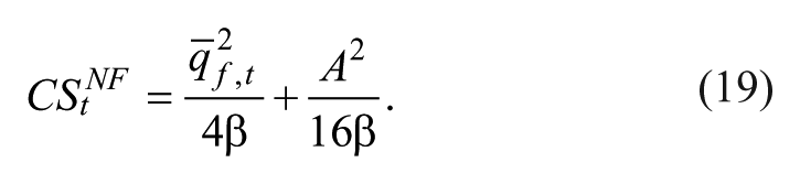
Only Fresh Product Is Available (No Refrigeration)

We assume that in an autarchic economy, there is a market demand for fresh bushmeat at period t, given by $q_{f,t}$ , that is related linearly and negatively to its price, $P_{f,t}$ according to the following:

$$D^{NF}:q_{f,t}=A-\mathrm{\beta }\cdot P_{f,t},$$

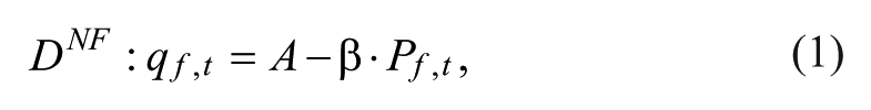
where A and β are parameters, f denotes fresh, t indicates time, and the superscript NF stands for “no freezer.” ¹³ The fresh bushmeat is sold in the market by a mamá who controls the whole market (we may call her a monopoly) and the bushmeat is supplied to the mamá by the hunters according to the quantity of bushmeat that they have caught in the current period. That quantity may be either large with a probability of 50% or small in quantity with the same probability. ¹⁴ Because the supply of bushmeat is totally inelastic, the price is determined by demand and the actual quantity that the mamá has available to sell. The revenue shares accruing to the mamá and the hunters are determined by mutual agreement. ¹⁵

Case 1.1: A shortage of fresh product

The first case occurs when the actual quantity of fresh bushmeat that arrives in period t at the market, ${\overline{q}}_{f,t}$ , is smaller than the optimal ${\widehat{q}}_{f,t}$ , which in our examples corresponds to the revenue maximizing quantity. ¹⁶ That is,

$${\overline{q}}_{f,t}<{\widehat{q}}_{f,t}.$$

In this case, all available units are sold, that is, the quantity of bushmeat consumed is equal to the quantity brought to market,

$$q_{f,t}={\overline{q}}_{f,t},$$

and, therefore, the equilibrium price is

$$P_{f,t}=\frac{A-{\overline{q}}_{f,t}}{\mathrm{\beta }}.$$

The profit function in this case is

$${\mathrm{\Pi }}_{t,1.1}=\frac{\left(A-{\overline{q}}_{f,t}\right)}{\mathrm{\beta }}\cdot {\overline{q}}_{f,t},$$

and the consumer surplus is computed as

$$C{S}_{t,1.1}=\frac{\frac{{\overline{q}}_{f,t}}{\mathrm{\beta }}\cdot {\overline{q}}_{f,t}}{2}=\frac{{\overline{q}}_{f,t}^2}{2\mathrm{\beta }}.$$

Figure 2 shows the equilibrium quantity and price, per the above derivation. Consumer surplus, labeled in the figure as such, is the area of the triangle under the demand curve but above the equilibrium price. It is understood to be the cumulative differences between what consumers were willing to pay for bushmeat, a point on the demand curve, and what they had to pay, the equilibrium price. The figure also shows producer surplus. The simplifying assumptions mean that producer surplus, revenue, and profit are all the same. Producer surplus is understood to be the cumulative sum of the difference between what the price sellers receive and the lowest price they would be willing to accept to cover variable costs.

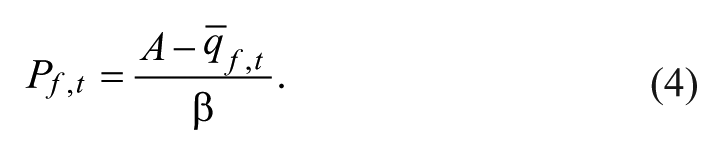
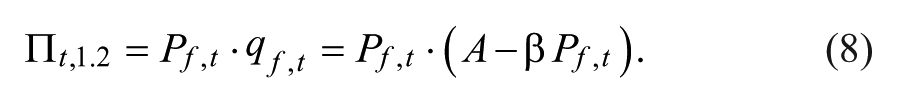
Case 1.2: An excess supply of fresh product

In the second case, the hunters bring too much bushmeat to the market and ${\overline{q}}_{f,t}>{\widehat{q}}_{f,t}$ , that is, the quantity brought to market exceeds the revenue maximizing quantity. Because the objective function of the mamás is revenue maximization, the desired and optimal quantity, ${\widehat{q}}_{f,t}$ , is defined as ${\widehat{q}}_{f,t}=\frac{A}{2},$ where the price elasticity for bushmeat is equal to -1, and total revenue is at its maximum. If ${\overline{q}}_{f,t}$ , the quantity that is supplied by the hunters, is larger than ${\widehat{q}}_{f,t}$ , all extra units beyond the revenue maximizing quantity, ${\overline{q}}_{f,t}-{\widehat{q}}_{f,t}$ , are destroyed because there is no use for spoiled bushmeat during the next market day (or period).

The equivalent expression to Equation 3 for this case is

$${\overline{q}}_{f,t}>{\widehat{q}}_{f,t}=q_{f,t}.$$

In this case, the profit function is

$${\mathrm{\Pi }}_{t,1.2}=P_{f,t}\cdot q_{f,t}=P_{f,t}\cdot \left(A-\mathrm{\beta }{P}_{f,t}\right).$$

The first-order condition (FOC) for revenue (profit) maximization with respect to price is

$$\frac{d{\mathrm{\pi }}_{t,1.2}}{d_{P_{f,t}}}=A-2\mathrm{\beta }{P}_{f,t}=0.$$

Thus, profit maximization leads to the following price and quantity values at the equilibrium

$$P_{f,t}=\frac{A}{2\mathrm{\beta }}$$

and

$${\widehat{q}}_{f,t}=A-\mathrm{\beta }\cdot \frac{A}{2\mathrm{\beta }}=\frac{A}{2}.$$

Profit is

$${\mathrm{\Pi }}_{t,1.2}=\frac{A^2}{4\mathrm{\beta }},$$

and the consumer surplus is

$$C{S}_{t,1.2}=\frac{{{\widehat{q}}^2}_{f,t}}{2\mathrm{\beta }}=\frac{A^2}{8\mathrm{\beta }}.$$

Figure 3 shows consumer and producer surplus as defined above. In addition, the figure also shows the quantity of over-harvesting that results from a lack of control of the supply chain. Finally, the figure shows the loss in economic welfare resulting from the fact that the mamá is not able to use price discrimination to sell all the carcasses brought to market. ¹⁷ This loss is the area of the trapezoid with the “Wasted Carcasses” label in it.

Figure 3.

The market for fresh bushmeat when there is excess supply.

As stated previously, we assume that only two scenarios are possible and, for simplicity, each of them occurs with the probability of 50%. Thus, we can derive the expected values of the important variables for the case of perishable items in the absence of refrigeration.

The expected price that is derived from Equations 4 and 10 above is

$$P_{f,t}^{NF}=\frac{1}{2}\cdot \left(\frac{3A-2{\overline{q}}_{f,t}}{2\mathrm{\beta }}\right),$$

the probability weighted average of the two prices shown in Figures 2 and 3.

The expected quantity that is derived from Equations 3 and 11 above is

$$q_{f,t}^{NF}=\frac{1}{2}\cdot \left({\overline{q}}_{f,t}+\frac{A}{2}\right),$$

the probability weighted average of the quantities shown in Figures 2 and 3. Indubitably, the probability weighted average is less than the revenue/profit maximizing quantity.

The expected profit when there is no refrigeration is also a probability weighted average

$${\mathrm{\Pi }}_t^{NF}=\frac{1}{2}\cdot {\mathrm{\Pi }}_{t,1.1}+\frac{1}{2}\cdot {\mathrm{\Pi }}_{t,1.2}.$$

Substituting from Equations 5 and 12 above, expected profit is

$${\mathrm{\Pi }}_t^{NF}=\frac{\left(A-{\overline{q}}_{f,t}\right)\cdot {\overline{q}}_{f,t}}{2\mathrm{\beta }}+\frac{A^2}{8\mathrm{\beta }}.$$

By the same token, we find the expected consumer surplus as

$$C{S}_t^{NF}=\frac{1}{2}\cdot C{S}_{t,1.1}+\frac{1}{2}\cdot C{S}_{t,1.2}.$$

Substituting from Equations 8 and 14, expected consumer surplus is, therefore,

$$C{S}_t^{NF}=\frac{{\overline{q}}_{f,t}^2}{4\mathrm{\beta }}+\frac{A^2}{16\mathrm{\beta }}.$$

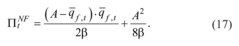
From Equations 17 and 19, we find that the expected total economic welfare that can be achieved when only fresh bushmeat is available in the market, and under supply fluctuation, is as follows:

$$W_t^{NF}={\mathrm{\Pi }}_t^{NF}+C{S}_t^{NF}=\frac{\left(2A-{\overline{q}}_{f,t}\right){\overline{q}}_{f,t}}{4\mathrm{\beta }}+\frac{3A^2}{16\mathrm{\beta }}.$$

Profit, consumer surplus, and welfare are all probability weighted averages of the amounts shown in the above figures. As an algebraic matter, all three probability weighted averages are less than they would be if the quantity supplied could be kept at ${\widehat{q}}_{f,t}$ with certainty. This suggests that managing the supply chain can positively affect economic welfare.

Both Fresh and Frozen/Stored Product Are Available

In this section, we investigate the scenario in which two substitute goods may be available in each period: both fresh and frozen bushmeat. This possibility may exist because the introduction of refrigeration enables the holding of bushmeat for an “extended time” (we assume for simplicity one period more).

Two separate, but dependent, demands exist as follows: the demand for fresh bushmeat, Equation 21 below, and the demand for frozen bushmeat carried over from the previous period, Equation 22 below.

The two separate but dependent demands exist in a non-symmetric way. The demand for fresh bushmeat, D_f, is affected negatively by the market price of the fresh bushmeat and positively by the market price of the old bushmeat (frozen from previous day or period) as follows:

$$D_f:q_{f,t}=\left(A-\frac{\mathrm{\alpha }B}{\mathrm{\gamma }}\right)-\mathrm{\beta }{P}_{f,t}+\mathrm{\alpha }{P}_{o,t}.$$

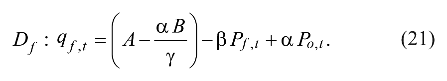
Here, the subscript “o” denotes old bushmeat carried over from the previous period. The symbols A, B, α, β, and γ are parameters. In this specification, an increase in the price of fresh meat will reduce the quantity of fresh meat demanded, and an increase in the price of “old” (frozen) meat, the substitute for fresh, will increase the quantity demanded of fresh meat.

However, the demand for old (frozen) bushmeat is affected negatively only by the price of the frozen bushmeat as follows:

$$D_o:q_{o,t}=B-\mathrm{\gamma }\cdot P_{o,t}.$$

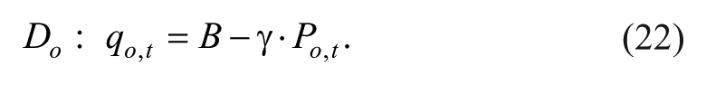
In this specification, consumers do not regard fresh meat to be a substitute for “old” meat. From Equations 21 and 22, we can define the actual interdependency between the demand for fresh bushmeat and for frozen bushmeat. If no frozen bushmeat is available, then the demand for fresh bushmeat stays the same as in Equation 1. However, if at a certain price of frozen bushmeat, $P_{o,t}$ , consumers buy some frozen bushmeat as a substitute for fresh, then the demand for fresh bushmeat is reduced. For this reason, we can say, based on Equation 22, that if $P_{o,t}=\frac{B}{\mathrm{\gamma }},$ then no one buys old bushmeat $\left(q_{o,t}=0\right)$ , and then $q_{f,t}$ of Equation 21 is the same as in Equation 1 in a market when only fresh bushmeat is available.

If $P_{o,t}<\frac{B}{\mathrm{\gamma }}$ , then some frozen bushmeat is purchased $\left(q_{o,t}>0\right)$ , and $q_{f,t}$ at Equation 21 is smaller than at Equation 1 at any given price $P_{f,t}$ . Hence, there is an asymmetric dependency between $q_{o,t}$ and $q_{f,t}$ .

The assumption here is that the price of fresh bushmeat does not affect the demand for frozen. This is assumed for simplicity and does not qualitatively affect the basic equilibrium and comparison with the first case above in which only fresh bushmeat is available. In the new case, several sub-cases should be considered.

Case 2.1: No frozen inventory, fresh supply and demand quantities are equal

Suppose that all fresh products are sold and no frozen items are carried over to a future period. Furthermore, in this case, no leftover items are available from a previous period such that $q_{o,t}=0$ , that is, no inventory of old items is available. It means that in this case, all arriving fresh units are sold, no old units are available from the previous day, and nothing is left for the following day.

This will happen if simultaneously the following inequalities hold:

$${\overline{q}}_{f,t-1}\le {\tilde{q}}_{f,t-1}\mathrm{and}{\overline{q}}_{f,t}\le {\tilde{q}}_{f,t},$$

that is, in the previous and the current period, the actual supply of units ${\overline{q}}_{f,t-1}$ and ${\overline{q}}_{f,t}$ are smaller than the optimal (revenue maximizing) quantities demanded in the previous and current periods, denoted as ${\tilde{q}}_{f,t-1}\mathrm{and}{\tilde{q}}_{f,t},$ respectively.

If $q_{o,t}=0,$ , that is, no frozen bushmeat is available in the current period, then the demand for fresh “returns” to the original demand of Equation 1. In this instance, all available units are sold, that is,

$$q_{f,t}={\overline{q}}_{f,t}$$

and, therefore, the equilibrium price is

$$P_{f,t}=\frac{A-{\overline{q}}_{f,t}}{\mathrm{\beta }}.$$

The profit function is again as follows:

$${\mathrm{\Pi }}_{t,2.1}=P_{f,t}\cdot {\overline{q}}_{f,t}$$

or

$${\mathrm{\Pi }}_{t,2.1}=\frac{\left(A-{\overline{q}}_{f,t}\right)}{\beta }.{\overline{q}}_{f,t},$$

and, therefore,

$$C{S}_{t,2.1}=\frac{{\overline{q}}_{f,t}^2}{2\mathrm{\beta }}.$$

For this case, the supply and demand figure would be identical to Figure 2.

Case 2.2: No frozen inventory, excess supply of fresh product

In this instance, it is again assumed that in the current period, no old (frozen) bushmeat is available from the previous period. However, the supply of fresh bushmeat in the current period is larger than the optimal quantity demanded (from the perspective of the seller) or

$${\overline{q}}_{f,t-1}\le {\tilde{q}}_{f,t-1}\mathrm{and}{\overline{q}}_{f,t}\ge {\tilde{q}}_{f,t}.$$

Because no old frozen units are left from the previous period, t − 1, $q_{o,t}=0$ , the demand for fresh bushmeat at period t is again given by Equation 1.

Thus, the profit function is

$${\mathrm{\Pi }}_{t,2.2}=P_{f,t}\cdot q_{f,t}=P_{f,t}\left(A-\mathrm{\beta }\cdot P_{f,t}\right).$$

The FOC we derive with respect to the current price at period t is

$$\frac{d{\mathrm{\Pi }}_{t,2.2}}{d{P}_{f,t}}=A-2\mathrm{\beta }{P}_{f,t}=0.$$

Thus, the price at the equilibrium is

$$P_{f,t}=\frac{A}{2\mathrm{\beta }}.$$

The quantity at the equilibrium is

$${\tilde{q}}_{f,t}=A-\mathrm{\beta }\cdot \frac{A}{2\mathrm{\beta }}=\frac{A}{2}.$$

The profit is

$${\mathrm{\Pi }}_{t,2.2}=\frac{A^2}{4\mathrm{\beta }},$$

and the consumer surplus is

$$C{S}_{t,2.2}=\frac{{\tilde{q}}_{f,t}^2}{2\mathrm{\beta }}=\frac{A^2}{8\mathrm{\beta }}.$$

Case 2.3: Excess demand for fresh with frozen inventory

This instance deals with the scenario where frozen units are left from the previous period, t – 1, such that ${\overline{q}}_{o,t}>0$ , since in the previous period ${\overline{q}}_{f,t-1}\ge {\tilde{q}}_{f,t-1}$ . However, the quantity of fresh bushmeat supplied in the current period, t, is less than the seller’s optimal, that is, ${\overline{q}}_{f,t}⩽{\tilde{q}}_{f,t}$ .

Here, we make an additional simplifying assumption that the frozen units left from the previous period, t – 1, is smaller than the seller’s optimal quantity for old (frozen) bushmeat in the current period, t.

Or,

$${\overline{q}}_{o,t}={\overline{q}}_{f,t-1}-{\tilde{q}}_{f,t-1}<{\tilde{q}}_{o,t}.$$

The reason for this assumption is very straightforward. In the long run, no seller holds more units of frozen bushmeat for the next period (or day) if he realizes that eventually he will destroy it at the end of that period due to a surplus of combined fresh and frozen bushmeat. It is better to destroy it earlier and save the holding cost of the frozen inventory. If we hold $q_{o,t}={\overline{q}}_{o,t}$ , then the price of the frozen item at the seller’s optimum is

$$P_{o,t}=\frac{B-{\overline{q}}_{o,t}}{\mathrm{\gamma }}$$

found by inverting Equation 22. Because there is no leftover fresh bushmeat from period t to be used as frozen bushmeat for period t + 1, we can say that

$$q_{f,t}={\overline{q}}_{f,t}.$$

Thus, the price of the fresh bushmeat at period t in equilibrium is

$$P_{f,t}=\frac{A-\frac{\mathrm{\alpha }B}{\mathrm{\gamma }}-{\overline{q}}_{f,t}+\frac{\mathrm{\alpha }}{\mathrm{\gamma }}\cdot \left(B-{\overline{q}}_{f,t}\right)}{\mathrm{\beta }}.$$

Or, by canceling terms,

$$P_{f,t}=\frac{A-{\overline{q}}_{f,t}-\frac{\mathrm{\alpha }}{\mathrm{\gamma }}\cdot {\overline{q}}_{o,t}}{\mathrm{\beta }}.$$

The circumstances of this case are summarized in Figures 4 and 5. The market for frozen meat is shown in Figure 4. It has an interpretation similar to that for Figure 2. The market for fresh meat is shown in Figure 5. The figure replicates the demand curve when there is no frozen meat available and includes the demand curve for fresh meat when frozen is available; note that there has been a leftward shift in demand due to the availability of a substitute. In Figure 5, it is apparent that the differences in consumer and producer surplus resulting from the demand shift may not be fully compensated by the consumer and producer surplus found in the frozen meat market; the net effect would depend on parameter values. However, Figure 5 shows unequivocally the decline in the harvest rate in the fresh market.

Figure 4.

The market for frozen bushmeat.

Figure 5.

The market for fresh bushmeat in the presence of frozen bushmeat carried over from the previous period.

The profit in Sub-case 2.3 will be

$${\mathrm{\Pi }}_{t,2.3}=P_{f,t}\cdot q_{f,t}+P_{o,t}\cdot q_{o,t}$$

or

$${\mathrm{\Pi }}_{t,2.3}=\frac{\left(A-{\overline{q}}_{f,t}-\frac{\mathrm{\alpha }}{\mathrm{\gamma }}\cdot {\overline{q}}_{o,t}\right)}{\mathrm{\beta }}\cdot {\overline{q}}_{f,t}+\frac{B-{\overline{q}}_{f,t}}{\mathrm{\gamma }}\cdot {\overline{q}}_{o,t}$$

or

$${\mathrm{\Pi }}_{t,2.3}=\frac{\left(A-{\overline{q}}_{f,t}\right)}{\mathrm{\beta }}\cdot {\overline{q}}_{f,t}+\left(B-{\overline{q}}_{o,t}-\frac{\mathrm{\alpha }{\overline{q}}_{o,t}}{\mathrm{\beta }}\right)\cdot \frac{{\overline{q}}_{o,t}}{\mathrm{\gamma }}.$$

The left term of the right-hand side of Equation 40 is

$\frac{\left(A-{\overline{q}}_{f,t}\right)}{\mathrm{\beta }}\cdot {\overline{q}}_{f,t}={\mathrm{\Pi }}_{t,2.1},$ that is, the profit of Case 2.2.

Therefore, we can conclude that the total profit at Sub-case 2.3 is larger than the profit of Case 2.1. Namely, ${\mathrm{\Pi }}_{t,2.3}>{\mathrm{\Pi }}_{t,2.1}.$

The consumer surplus of Case 2.3 is a summation of consumers’ surplus (CS) derived from fresh and frozen items as follows:

$$C{S}_{t,2.3}=C{S}_{f,t}+C{S}_{o,t}=\frac{{\overline{q}}_{f,t}^2}{2\mathrm{\beta }}+\frac{{\overline{q}}_{o,t}^2}{2\mathrm{\gamma }}.$$

The affect on consumer surplus is ambiguous, but there is an increase in profit to the vendors.

Case 2.4: Frozen inventory, excess supply of fresh product

In Case 2.4, the seller faces a scenario in which old frozen units are left from period t – 1, but at the same time, some fresh units from the current period t are chosen to be carried over and sold by the seller as frozen items at period t + 1. This occurs if the quantity of available bushmeat exceeds the sales maximizing quantity in both the prior and current period: ${\overline{q}}_{f,t-1}>{\tilde{q}}_{f,t-1}$ and ${\overline{q}}_{f,t}\ge {\tilde{q}}_{f,t}.$

The same assumption of Case 2.3 that the quantity of old bushmeat is less than the revenue maximizing quantity is used for a similar reason. Hence,

$${\overline{q}}_{o,t}={\overline{q}}_{f,t-1}-{\tilde{q}}_{f,t-1}<{\tilde{q}}_{0,t}.$$

In this case, the actual quantity of the frozen item is

$$q_{o,t}={\overline{q}}_{o,t}.$$

Thus, the equilibrium price of a frozen unit is

$$P_{o,t}=\frac{B-{\overline{q}}_{o,t}}{\mathrm{\gamma }}.$$

The total profit of the seller who sells all frozen units and fresh units at period t adds up to the following profit function:

$${\mathrm{\Pi }}_{t,2.4}=P_{f,t}\cdot q_{f,t}+P_{o,t}\cdot q_{o,t}$$

or

$$\begin{array}{l}{\mathrm{\Pi }}_{t,2.4}=\left[A-\frac{\mathrm{\alpha }B}{\mathrm{\gamma }}-\mathrm{\beta }\cdot P_{f,t}+\frac{\mathrm{\alpha }}{\mathrm{\gamma }}\cdot \left(B-{\overline{q}}_{o,t}\right)\right]\cdot \\ P_{f,t}+\frac{\left(B-{\overline{q}}_{o,t}\right)\cdot {\overline{q}}_{o,t}}{\mathrm{\gamma }}.\end{array}$$

Because the frozen unit’s price is given, the seller has to maximize profit and derives the FOC only with respect to the price of fresh bushmeat as follows:

$$\frac{d{\mathrm{\Pi }}_{t,2.4}}{d{P}_{f,t}}=A-\frac{\mathrm{\alpha }B}{\mathrm{\gamma }}-2\mathrm{\beta }{P}_{f,t}+\frac{\mathrm{\alpha }B}{\mathrm{\gamma }}-\frac{\mathrm{\alpha }\cdot {\overline{q}}_{o,t}}{\mathrm{\gamma }}=0.$$

From the FOC, we find the optimal price of a fresh unit, $P_{ft}$ , the optimal quantity, ${\tilde{q}}_{f,t}$ , and profit in Case 2.4 as follows:

$$P_{f,t}=\frac{A}{2\mathrm{\beta }}-\frac{\mathrm{\alpha }{\overline{q}}_{o,t}}{2\mathrm{\beta }\mathrm{\gamma }},$$

$${\tilde{q}}_{f,t}=A-\frac{\mathrm{\alpha }B}{\mathrm{\gamma }}-\mathrm{\beta }\cdot \left(\frac{A}{2\mathrm{\beta }}-\frac{\mathrm{\alpha }{\overline{q}}_{o,t}}{2\mathrm{\beta }\mathrm{\gamma }}\right)+\frac{\mathrm{\alpha }}{\mathrm{\gamma }}\cdot \left(B-{\overline{q}}_{o,t}\right),$$

or

$${\tilde{q}}_{f,t}=\frac{A}{2}-\frac{\mathrm{\alpha }{\overline{q}}_{o,t}}{2\mathrm{\gamma }}.$$

The profit is

$${\mathrm{\Pi }}_{t,2.4}=\frac{1}{\mathrm{\beta }}\cdot {\left(\frac{A}{2}-\frac{\mathrm{\alpha }{\overline{q}}_{o,t}}{2\mathrm{\gamma }}\right)}^2+\frac{\left(B-{\overline{q}}_{o,t}\right)\cdot {\overline{q}}_{o,t}}{\mathrm{\gamma }}.$$

The consumer surplus gained in Case 2.4 is

$$C{S}_{t,2.4}=\frac{{\left(\frac{A}{2}-\frac{\mathrm{\alpha }{\overline{q}}_{o,t}}{2\mathrm{\gamma }}\right)}^2}{2\mathrm{\beta }}+\frac{{{\overline{q}}_{o,t}}^2}{2\mathrm{\gamma }}.$$

As was done earlier when no frozen units are available and the events of small and large quantities of fresh bushmeat supplied to the market occur with equal probability, we compute the expected value for price, quantity, profit, consumer surplus, and welfare. Each of the four sub-cases of Case 2 has a probability of occurrence of .25 for the same reasoning as was used in the sub-cases of Case 1; economy of notation without a qualitative change in conclusions. Thus, the expected price of fresh units when freezing is available (superscript F), ${P_{f,t}}^F$ , is

$$P_{f,t}^F=\frac{1}{4}\cdot \left[\begin{array}{l}\frac{A-{\overline{q}}_{f,t}}{\mathrm{\beta }}+\frac{A}{2\mathrm{\beta }}+\frac{A-{\overline{q}}_{f,t}-\frac{\mathrm{\alpha }}{\mathrm{\gamma }}\cdot {\overline{q}}_{o,t}}{\mathrm{\beta }}+\\ \frac{A}{2\mathrm{\beta }}-\frac{\mathrm{\alpha }{\overline{q}}_{o,t}}{2\mathrm{\beta }\mathrm{\gamma }}\end{array}\right]$$

or

$$P_{f,t}^F=\frac{1}{4}\cdot \left(\frac{3A-2{\overline{q}}_{f,t}}{\mathrm{\beta }}-\frac{3\mathrm{\alpha }{\overline{q}}_{o,t}}{2\mathrm{\beta }\mathrm{\gamma }}\right).$$

The expected quantity of fresh bushmeat is

$$q_{f,t}^F=\frac{1}{4}\cdot \left({\overline{q}}_{f,t}+\frac{A}{2}+{\overline{q}}_{f,t}+\frac{A}{2}-\frac{\mathrm{\alpha }{\overline{q}}_{o,t}}{2\mathrm{\gamma }}\right)$$

or

$$q_{f,t}^F=\frac{1}{4}\cdot \left(A+2{\overline{q}}_{f,t}-\frac{\mathrm{\alpha }{\overline{q}}_{o,t}}{2\mathrm{\gamma }}\right).$$

The expected price of frozen (old) units is

$$P_{o,t}^F=\frac{1}{4}\cdot \left(\frac{B}{\mathrm{\gamma }}+\frac{B}{\mathrm{\gamma }}+\frac{B-{\overline{q}}_{o,t}}{\mathrm{\gamma }}+\frac{B-{\overline{q}}_{o,t}}{\mathrm{\gamma }}\right)$$

or

$$P_{o,t}^F=\frac{B}{\mathrm{\gamma }}-\frac{{\overline{q}}_{o,t}}{2\mathrm{\gamma }}.$$

Although the expected quantity of frozen units sold is

$$q_{o,t}^F=\frac{1}{4}\cdot \left(0+0+{\overline{q}}_{o,t}+{\overline{q}}_{o,t}\right)=\frac{{\overline{q}}_{o,t}}{2},$$

the total expected profit from the four sub-cases of Case 2 is

$${\mathrm{\Pi }}_{f,t}^F=\frac{1}{4}\cdot {\mathrm{\Pi }}_{t,2.1}+\frac{1}{4}\cdot {\mathrm{\Pi }}_{t,2.2}+\frac{1}{4}\cdot {\mathrm{\Pi }}_{t,2.3}+\frac{1}{4}\cdot {\mathrm{\Pi }}_{t,2.4}$$

or

$${\mathrm{\Pi }}_{f,t}^F=\frac{1}{4}\cdot \left[\begin{array}{l}\frac{\left(A-{\overline{q}}_{f,t}\right)}{\mathrm{\beta }}\cdot {\overline{q}}_{f,t}+\frac{A^2}{4\mathrm{\beta }}+\frac{\left(A-{\overline{q}}_{f,t}\right)}{\mathrm{\beta }}{\overline{q}}_{f,t}+\\ \left(B-{\overline{q}}_{o,t}-\frac{\mathrm{\alpha }{\overline{q}}_{o,t}}{\mathrm{\beta }}\right)\cdot \frac{\mathrm{\alpha }{\overline{q}}_{o,t}}{\mathrm{\gamma }}+\\ +\frac{1}{\mathrm{\beta }}\cdot {\left(\frac{A}{2}-\frac{\mathrm{\alpha }{\overline{q}}_{o,t}}{2\mathrm{\gamma }}\right)}^2+\frac{\left(B-{\overline{q}}_{o,t}\right){\overline{q}}_{o,t}}{\mathrm{\gamma }}\end{array}\right]$$

or

$${\mathrm{\Pi }}_{f,t}^F=\frac{1}{4}\cdot \left[\begin{array}{l}\frac{\left(A-{\overline{q}}_{f,t}\right)}{\mathrm{\beta }}\cdot 2{\overline{q}}_{f,t}+\frac{A^2}{4\mathrm{\beta }}+\\ \left(2B-2{\overline{q}}_{o,t}-\frac{\mathrm{\alpha }{\overline{q}}_{o,t}}{\mathrm{\beta }}\right)\cdot \\ \frac{{\overline{q}}_{o,t}}{\mathrm{\gamma }}+\frac{1}{\mathrm{\beta }}\cdot {\left(\frac{A}{2}-\frac{\mathrm{\alpha }{\overline{q}}_{o,t}}{2\mathrm{\gamma }}\right)}^2\end{array}\right].$$

As a result, the total expected consumer surplus and social welfare are

$$C{S}_t^F=\frac{1}{4}\cdot \left[\frac{{\overline{q}}_{f,t}^2}{\mathrm{\beta }}+\frac{A^2}{8\mathrm{\beta }}+\frac{{\overline{q}}_{o,t}^2}{\mathrm{\gamma }}+\frac{{\left(\frac{A}{2}-\frac{\mathrm{\alpha }{\overline{q}}_{o,t}}{2\mathrm{\gamma }}\right)}^2}{2\mathrm{\beta }}\right]\mathrm{and}$$

$$W_t^F=\frac{1}{4}\cdot \left[\begin{array}{l}\frac{\left(2A-{\overline{q}}_{f,t}\right)\cdot {\overline{q}}_{f,t}}{\mathrm{\beta }}+\frac{3A^2}{8\mathrm{\beta }}+\\ \left(2B-{\overline{q}}_{o,t}-\frac{\mathrm{\alpha }{\overline{q}}_{o,t}}{\mathrm{\beta }}\right)\cdot \\ \frac{{\overline{q}}_{o,t}}{\mathrm{\gamma }}+\frac{3}{2\mathrm{\beta }}{\left(\frac{A}{2}-\frac{\mathrm{\alpha }{\overline{q}}_{o,t}}{2\mathrm{\gamma }}\right)}^2\end{array}\right].$$

Comparison of Outcomes

The results of Cases 1.1 and 1.2 versus Cases 2.1 through 2.4 above, only fresh bushmeat in the market versus both fresh and frozen bushmeat in the market, can be used to compare the values of expected profits (producer surplus), expected consumer surplus, and expected economic welfare to gain better insight into the value added of the “new” refrigeration technology in a market with stochastic supply fluctuations. The first comparison is related to the expected quantity of fresh units that are sold in an environment where only fresh units are available versus an environment in which both fresh and frozen units are available. We ask whether the quantity of fresh bushmeat in a market with no refrigeration, $q_{f,t}^{NF},$ is smaller or larger than the expected fresh quantity sold, $q_{f,t}^F,$ when some units can be held over under refrigeration. That is, we are interested in the direction of the following inequality:

$$\begin{array}{l}{q}_{f,t}^{NF}=\frac{1}{2}\cdot \left({\overline{q}}_{f,t}+\frac{A}{2}\right)\frac{>}{<}\frac{1}{4}\cdot \\ \left(A-2{\overline{q}}_{f,t}-\frac{\mathrm{\alpha }{\overline{q}}_{o,t}}{2\mathrm{\gamma }}\right)=q_{f,t}^F.\end{array}$$

On the left-hand side of the inequality is expected quantity when there is no refrigeration. On the right-hand side of the inequality is the expected quantity of fresh meat when there is refrigeration that allows carry over from one period to the next. Because $\frac{\mathrm{\alpha }{\overline{q}}_{o,t}}{2\mathrm{\gamma }}>0,$ when the freezing process is available, the seller may postpone some sales and convert fresh units to frozen units. Therefore, it must be that $q_{f,t}^{NF}>q_{f,t}^F.$ The important conclusion from the model is that because freezing a unit is an alternative, less fresh units will be sold than under a regime in which frozen units are not available. Unequivocally, we know that bushmeat takeoff is reduced.

Similarly, when frozen units are sold as well as fresh units, we want to compare the effect of the technological improvement on prices. We are interested in the direction of the inequality

$$\begin{array}{l}{P}_{f,t}^{NF}=\frac{1}{2}\cdot \left(\frac{3A-2{\overline{q}}_{f,t}}{2\mathrm{\beta }}\right)\frac{>}{<}\frac{1}{4}\cdot \\ \left(\frac{3A-2{\overline{q}}_{f,t}}{\mathrm{\beta }}-\frac{3\mathrm{\alpha }{\overline{q}}_{o,t}}{2\mathrm{\beta }\mathrm{\gamma }}\right)=P_{f,t}^F.\end{array}$$

Because $\frac{3\mathrm{\alpha }{\overline{q}}_{o,t}}{2\mathrm{\beta }\mathrm{\gamma }}>0,$ we find, as expected, that $P_{f,t}^{NF}>P_{f,t}^F.$ That is, when the freezing process is not available, the price of the fresh bushmeat is higher.

From the standpoint of species preservation, the important result is that $P_{f,t}^{NF}>P_{f,t}^F$ and $q_{f,t}^{NF}>q_{f,t}^F.$ In any period t, the price of fresh bushmeat is lower, and the harvest rate is lower in a regime with refrigeration (superscript F) than in a regime without refrigeration (superscript NF). The intuition is illustrated in Figure 5 by the leftward shift in the demand for fresh bushmeat.

The next interesting question is how many units will be sold if only fresh units are available and no frozen units are sold because of the unavailability of the freezing process for legal or other reasons; sellers are not allowed or can’t sell frozen units. We may expect that by allowing some units to be frozen and carried forward, the sellers have more flexibility and may sell more and destroy fewer leftovers (units), in comparison with the case when only fresh units can be sold.

By Equations 15, 55, and 58, above, we find an interesting result regarding the total quantity of bushmeat traded in the marketplace. The relevant comparison is as follows:

$$\frac{1}{2}\cdot \left({\overline{q}}_{f,t}+\frac{A}{2}\right)\frac{>}{<}\frac{1}{4}\cdot \left(A+2{\overline{q}}_{f,t}-\frac{\mathrm{\alpha }{q}_{o,t}}{2\mathrm{\gamma }}\right)+\frac{1}{2}{\overline{q}}_{o,t}.$$

If $\mathrm{\alpha }>4\mathrm{\gamma }$ (meaning that the preference for fresh bushmeat is quite weak relative to the sensitivity of demand for frozen units, found by manipulating Equation 66 when no units are carried forward), then the number of units sold in the market when only fresh can be sold is larger than the number of fresh units sold in the case where frozen inventory also can be supplied, in comparison with total unit sales when both fresh and frozen can be brought to market, that is, $q_{f,t}^{NF}>\left(q_{f,t}^F+q_{o,t}^F\right).$ From the standpoint of preservation of species, this is a happy result, because the total consumption of the endangered species has been reduced below the rate when there is no refrigeration.

The opposite occurs only when $\mathrm{\alpha }<4\mathrm{\gamma },$ then $q_{f,t}^{NF}<\left(q_{f,t}^F+q_{o,t}^F\right);$ that is, total units sold is greater when there is refrigeration than when there is not. On the surface, this result does not appear to be auspicious for the endangered species. However, this result also induces reduced pressure on the species being harvested because, from Equations 64 and 65, $q_{f,t}^{NF}>q_{f,t}^F,$ the increased total consumption must result from the carryover of inventory from one period to another rather than an increased harvest. In summary, although current period total consumption is higher with refrigeration, the harvest rate is still below the rate when there is no refrigeration: $q_{f,t}^{NF}>q_{f,t}^F.$

The comparison of profits with and without refrigeration (as well as consumer surplus and social welfare discussed below) leads to an ambiguous relationship:

$$\begin{array}{l}{\mathrm{\Pi }}_t^{NF}=\frac{\left(A-{\overline{q}}_{f,t}\right){\overline{q}}_{f,t}}{2\mathrm{\beta }}+\frac{A^2}{8\mathrm{\beta }}\frac{>}{<}\frac{1}{4}\cdot \\ [\frac{\left(A-{\overline{q}}_{f,t}\right)\cdot 2{\overline{q}}_{f,t}}{\mathrm{\beta }}+\frac{A^2}{4\mathrm{\beta }}+\\ +\begin{array}{l}\left(2B-2{\overline{q}}_{o,t}-\frac{\mathrm{\alpha }{\overline{q}}_{o,t}}{\mathrm{\beta }}\right)\cdot \\ \frac{{\overline{q}}_{o,t}}{\mathrm{\gamma }}+\frac{1}{\mathrm{\beta }}{\left(\frac{A}{2}-\frac{\mathrm{\alpha }{\overline{q}}_{o,t}}{2\mathrm{\gamma }}\right)}^2\end{array}]={\mathrm{\Pi }}_t^F.\end{array}$$

The gap between the expected profits of the two cases leads to

$$\begin{array}{l}{\mathrm{\Pi }}_t^F-{\mathrm{\Pi }}_t^{NF}=\left(2B-2{\overline{q}}_{o,t}-\frac{\mathrm{\alpha }{\overline{q}}_{o,t}}{\mathrm{\beta }}\right)\cdot \\ \frac{{\overline{q}}_{o,t}}{\mathrm{\gamma }}+\frac{{\mathrm{\alpha }}^2{\overline{q}}_{o,t}^2}{16{\mathrm{\gamma }}^2}-\frac{\mathrm{\alpha }{\overline{q}}_{o,t}A}{8\mathrm{\gamma }}\end{array}$$

or

$${\mathrm{\Pi }}_t^F-{\mathrm{\Pi }}_t^{NF}=\left[2B-\frac{\mathrm{\alpha }A}{8}-\left(2+\frac{\mathrm{\alpha }}{\mathrm{\beta }}-\frac{{\mathrm{\alpha }}^2}{16\mathrm{\gamma }}\right)\cdot {\overline{q}}_{o,t}\right]\cdot \frac{{\overline{q}}_{o,t}}{\mathrm{\gamma }},$$

where the term in the bracket may be positive or negative, indicating no fixed relationship between markets with and without available frozen inventory. In the same way, we compare consumer surplus of both cases as follows:

$$\begin{array}{l}C{S}_t^{NF}=\frac{{\overline{q}}_{f,t}^2}{4\mathrm{\beta }}+\frac{A^2}{16\mathrm{\beta }}\frac{>}{<}\frac{1}{4}\cdot \\ \left[\frac{{\overline{q}}_{f,t}^2}{\mathrm{\beta }}+\frac{A^2}{8\mathrm{\beta }}+\frac{{\overline{q}}_{o,t}^2}{\mathrm{\gamma }}+\frac{{\left(\frac{A}{2}-\frac{\mathrm{\alpha }{\overline{q}}_{o,t}}{2\mathrm{\gamma }}\right)}^2}{2\mathrm{\beta }}\right]=C{F}_t^F\end{array}$$

or

$$C{F}_t^F-C{S}_t^{NF}=\frac{{\overline{q}}_{o,t}^2}{4\mathrm{\gamma }}-\frac{\mathrm{\alpha }{\overline{q}}_{o,t}A}{16\mathrm{\beta }\mathrm{\gamma }}+\frac{{\mathrm{\alpha }}^2{\overline{q}}_{o,t}^2}{32\mathrm{\beta }{\mathrm{\gamma }}^2}$$

or

$$C{F}_t^F-C{S}_t^{NF}=\left[\left(1+\frac{{\mathrm{\alpha }}^2}{8\mathrm{\beta }\mathrm{\gamma }}\right)\cdot {\overline{q}}_{o,t}-\frac{\mathrm{\alpha }}{4\mathrm{\beta }}\cdot A\right]\frac{{\overline{q}}_{o,t}}{4\mathrm{\gamma }}.$$

The differences can be again either positive or negative, as determined by the parameter values in the square brackets.

As a result of the ambiguity of profit and consumer surplus comparisons, we find the same ambiguous results with respect to the total expected welfare of both cases as follows:

$$\begin{array}{l}{W}_t^{NF}=\frac{\left(2A-{\overline{q}}_{f,t}\right)\cdot {\overline{q}}_{f,t}}{4\mathrm{\beta }}+\frac{3A^2}{16\mathrm{\beta }}\frac{>}{<}\frac{1}{4}\cdot \\ [\frac{\left(2A-{\overline{q}}_{f,t}\right)\cdot {\overline{q}}_{f,t}}{\mathrm{\beta }}+\frac{3A^2}{8\mathrm{\beta }}+\\ +\begin{array}{l}\left(2B-{\overline{q}}_{o,t}-\frac{\mathrm{\alpha }{\overline{q}}_{o,t}}{\mathrm{\beta }}\right)\cdot \frac{{\overline{q}}_{o,t}}{\mathrm{\gamma }}+\frac{3}{2\mathrm{\beta }}\cdot \\ {\left(\frac{A}{2}-\frac{\mathrm{\alpha }{\overline{q}}_{o,t}}{2\mathrm{\gamma }}\right)}^2\end{array}]=W_t^F\end{array}$$

or

$$\begin{array}{l}{W}_t^F-W_t^{NF}=\left(2B-{\overline{q}}_{o,t}-\frac{\mathrm{\alpha }{\overline{q}}_{o,t}}{\mathrm{\beta }}\right)\cdot \\ \frac{{\overline{q}}_{o,t}}{4\mathrm{\gamma }}-\frac{3\mathrm{\alpha }{\overline{q}}_{o,t}A}{16\mathrm{\beta }\mathrm{\gamma }}+\frac{3{\mathrm{\alpha }}^2{\overline{q}}_{o,t}^2}{32\mathrm{\beta }{\mathrm{\gamma }}^2}\end{array}$$

or

$$W_t^F-W_t^{NF}=\left[2B-\frac{3\mathrm{\alpha }A}{4\mathrm{\beta }}-\left(1+\frac{\mathrm{\alpha }}{\mathrm{\beta }}-\frac{3{\mathrm{\alpha }}^2}{8\mathrm{\beta }\mathrm{\gamma }}\right)\cdot {\overline{q}}_{o,t}\right]\cdot \frac{{\overline{q}}_{o,t}}{4\mathrm{\gamma }}.$$

The differences again can be positive or negative as determined by the sign of the term in square brackets.

This leads us to a very important conclusion that needs emphasizing: Technological improvement does not necessarily lead to a pareto improvement scenario when the sole consideration is economic efficiency. Therefore, consumers or suppliers do not necessarily seek the technologic improvement. However, the value to society, which is of little concern to consumers and sellers as individuals, of the reduced harvest rate of the endangered species may be more than enough to offset the strict consideration of economic efficiency.

At this stage, we wish to undertake comparisons between CS, producer surplus, Π, and total social welfare, W, between the frozen and non-frozen scenarios and how these comparisons and differences are affected by changes in the two parameters α and β.

The parameter α represents the degree of substitutability between the frozen and fresh units that consumers buy. When α is relatively small, it indicates a strong preference for freshness. People may perceive fresh bushmeat as a product that cannot be substituted by frozen bushmeat. In this scenario, the cross price effect will be small, that is, when the value of α is small, a decrease in the price of frozen bushmeat will not lead to a large reduction in the quantity demanded of fresh bushmeat.

In our model, we assume that a decrease in α reduces the demand for fresh items as well as the consumer surplus because frozen items are also available. As a result, the profits of the sellers from the sale of fresh and frozen items are larger than in the case where only fresh items are available. However, as α becomes larger, that is, there is a greater degree of crossover between fresh and frozen, the sellers gain less profits than what they achieve when the frozen item is unavailable.

If both consumer surplus and profits shrink with an increase in α, then it has the same effect with respect to welfare, W. The freezing innovation may reduce society’s economic welfare, especially when fresh and frozen are close substitutes.

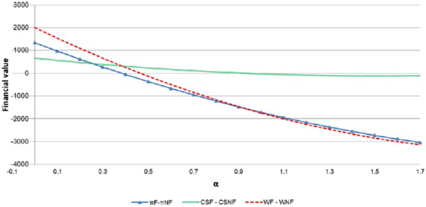
In Figures 6 and 7, consumer surplus, profit, and welfare are decreasing in the parameter α. Figure 6 permits side-by-side comparisons of consumer surplus, producer surplus, and economic welfare in the presence or absence of refrigeration. In taking the differences in the appropriate pairs from Figure 6, Figure 7 illustrates the values of α for which either buyers or sellers or the combination of the two have an interest in introducing refrigeration. For low values of α, less than ~ .4, consumer surplus, profit, and welfare are greater when there is refrigeration than when there is not. That is, it is only when the preference for freshness is strong that anyone has an incentive to introduce refrigeration. For .4 < α < .5, consumer surplus is positive but producer surplus is negative, so there will be a conflict between the two sides of the market regarding the adoption of refrigeration.

Figure 6.

Changes of a coefficient on the total values of CS, π, and W frozen vs. no frozen.

Figure 7.

Changes of a coefficient on the values’ difference between frozen and no frozen scenarios of CS, π, and W.

Similarly, in Figures 8 and 9, we analyze the effect of a change in the β coefficient, which represents the absolute change in quantity demanded resulting from a change in fresh bushmeat’s own price. A larger β reduces the quantity demanded. Figures 8 and 9 show that when demand is inelastic due to a small value for β, say less than .2, all three variables CS, Π, and W are larger and the market without the new freezing innovation is preferable. For .2 < β < .4, consumers want refrigeration, but producers do not. However, when the coefficient β approaches moderate and larger values, say β > .4, then the freezing innovation implementation is preferable from the standpoint of sustainability, although the total values of CS, Π, and W are significantly smaller and neither buyers nor sellers want to adopt refrigeration.

Figure 8.

Changes of a β coefficient on the total values of CS, π, and W frozen vs. no frozen.

Figure 9.

Changes of a β coefficient on the values’ differences between frozen and no frozen scenarios of CS, π, and W.

Conclusion

In the course of the last 25 years, the wildlife of Bioko Island, Equatorial Guinea, has come under increasing hunting pressure as a result of newfound oil wealth, road construction, and population change. The consequence has been unsustainable harvest rates and the possible extirpation of some species (Cronin, Riaco, Linder, & Hearn, 2016). Morra et al. (2009) modeled the bargaining process in the bushmeat market in Malabo. It was found that the weak bargaining position of the sellers of bushmeat, at least in part due to the lack of refrigeration, resulted in low prices and little control of the supply chain. In that paper, it was speculated that the introduction of refrigeration would reduce hunting pressure. In this article, a model of the introduction of refrigeration shows that it can indeed slow harvest rates. Refrigeration allows the carrying forward from one period to the next of the excess supply of bushmeat, this puts downward pressure on the demand for fresh bushmeat. In the post-refrigeration era, the model shows that the harvest of fresh bushmeat will fall. Indeed, the combined total consumption of stored and fresh bushmeat will fall. However, there is an important caveat. Depending on model parameters, the introduction of refrigeration can result in a reduction of consumer surplus and producer surplus under certain circumstances such that both are lower, or the total may be lower, in the post-technology era than in the pre-technology era. In those circumstances, there is no incentive for private parties to introduce refrigeration, and harvest rates will not fall. Furthermore, unless private entities attach economic value to biodiversity, the incentives would not change and the introduction of refrigeration might require intervention by a third party. ¹⁸