Sage Journals: Discover world-class research

Abstract

Estimation by minimizing the sum of squared residuals is a common method for parameters of regression functions; however, regression functions are not always known or of interest. Maximizing the likelihood function is an alternative if a distribution can be properly specified. However, cases can arise in which a regression function is not known, no additional moment conditions are indicated, and we have a distribution for the random quantities, but maximum likelihood estimation is difficult to implement. In this article, we present the least squared simulated errors (LSSE) estimator for such cases. The conditions for consistency and asymptotic normality are given. Finite sample properties are investigated via Monte Carlo experiments on two examples. Results suggest LSSE can perform well in finite samples. We discuss the estimator’s limitations and conclude that the estimator is a viable option. We recommend Monte Carlo investigation of any given model to judge bias for a particular finite sample size of interest and discern whether asymptotic approximations or resampling techniques are preferable for the construction of tests or confidence intervals.

Keywords

least squares analysis nonlinear regression Monte Carlo methods simulation experiments

Introduction

Minimizing the sum of squared residuals is a common estimation method for regression functions, but regression functions are not always known or of interest, particularly when motivated by an underlying structural equation. If a distribution for random terms is specified, maximizing the likelihood function is an alternative estimation method that does not require an explicit regression function. However, cases can arise in which the regression function is not known, no additional moment conditions are indicated, and we have a distribution for the random quantities, but maximum likelihood estimation is difficult to implement. This article presents a simulated moments estimation method for such cases similar to the simulation-based extensions of other common estimators such as maximum simulated likelihood and simulated scores (Gourieroux & Monfort, 1993; McFadden, 1989; McFadden & Ruud, 1994; Stern, 1997; Train, 2003).

Consider a simple example in which a response y to exogenous variable x for each person w in a population of interest is modeled as $y_{w} = α + {(β \cdot x_{w})}^{δ_{w}}$ with x≥ 0, α> 0, β> 0, and δ∈ (0,1). The model implies an idealized relation y = α + β·x from which each person’s response relationship is modified to a curve by a personal parameter δ_w. Suppose the data generating process implies a probability model for each data observation i as $y_{i} = α + {(β \cdot x_{i})}^{δ_{i}}$ with δ_i denoting a latent (i.e., unmeasured) variable (see Figure 1 for examples of this function). The regression equation is not known explicitly, so minimizing the sum of squared errors is not immediately applicable. For the same reason, the parameterization for the conditional likelihood function for y is not explicit. The least squared simulated errors (LSSE) estimator presented below provides a simple means of estimating such models.

Figure 1.

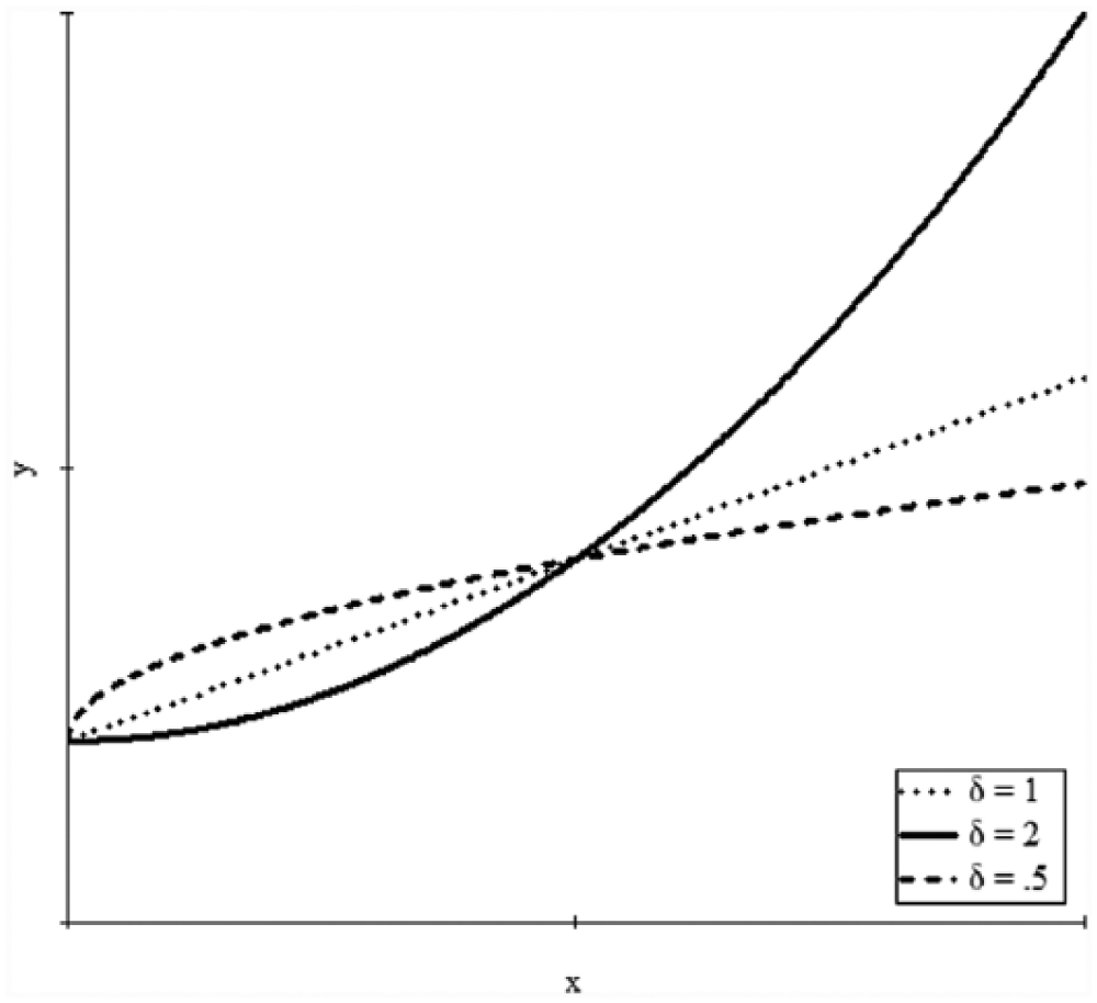
Graphs of the equation y = 1 + (0.2·x)^δ for three values of δ.

In the following section, we present the estimator and its asymptotic properties. We then present a Monte Carlo investigation of finite sample properties via two examples. In the final section, we discuss implications and limitations of the LSSE estimator.

LSSE

To understand the LSSE estimator and its asymptotic properties, consider a response or dependent variable y, for an observation i, expressed as a function g of observed covariates x, unobserved quantities η, and model parameters θ= (β′, φ′)′:

y_{i} = g (x_{i}, η_{i} | β),

with

η_{i} ~ F_{ϕ} .

The function g represents the structural model under consideration (e.g., a theory-derived model of an underlying mechanism, not a regression function), and the unobserved quantity η_i has distribution F_φ, with parameters φ. Assuming that the conditional expectation of y exists, the relationship y_i = E(y_i|x_i) + ε_i can be expressed as

y_{i} = \int g (x_{i}, η_{i} | β) d F_{ϕ} + ε_{i},

where the integral represents the regression and ε_i is the regression error term having expectation of 0.

Monte Carlo integration provides an unbiased estimator, ${\hat{y}}_{i} (θ)$ , of the regression function E(y_i|x_i) (Robert & Casella, 2004; Train, 2003). The Monte Carlo estimate for observation i is the average of the function g evaluated at x_i across the R samples of η drawn from the distribution F_φ:

{\hat{y}}_{i} (θ) = \frac{1}{R} \sum_{r = 1}^{R} g (x_{i}, η_{r} (ϕ) | β) .

The term η_r represents the rth random drawn from distribution F_φ.

Denoting the simulated residual as

{\hat{e}}_{i} (θ) = y_{i} - {\hat{y}}_{i} (θ),

and, for sample size N, denoting the corresponding N× 1 sample vector of simulated residuals as ${\hat{e}}_{R} (θ)$ then the definition of the LSSE estimator is given as follows.

For N observations and N×N positive definite matrix M, the LSSE estimator is

\hat{θ} = \underset{θ}{arg min} ({\hat{e}}_{R} {(θ)}^{'} \cdot M \cdot {\hat{e}}_{R} (θ)) .

The LSSE estimator is the value of θ that minimizes the sample residual vector relative to the metric determined by M. For M, an identity matrix (i.e., a square matrix with ones in the diagonal elements and zeroes in the off-diagonal elements), the estimator simply minimizes the sum of squared simulated errors:

\hat{θ} = \underset{θ}{arg min} ({\hat{e}}_{R} {(θ)}^{'} \cdot {\hat{e}}_{R} (θ)) .

The large-sample properties of the LSSE estimator are established by showing that the LSSE estimator is asymptotically equivalent to the standard nonlinear least squares estimator (NLS). Essentially, for each property considered, it can be shown that the key quantities of interest can be expressed as the standard NLS estimator plus a simulation bias that is asymptotically zero.

As shown in Appendix A, we see that if the assumptions underlying consistency and normality of the NLS estimator hold for the model under consideration, then for increasing number of Monte Carlo iterations used in the numeric integration (R) and increasing sample size (N), the LSSE estimator is consistent, and if R rises faster than the square root of N, the LSSE estimator has an asymptotic normal distribution. Essentially, as R and N go to infinity with R rising faster than the square root of N, the LSSE estimator is asymptotically equivalent to the NLS (Seber & Wild, 2003). This is somewhat comforting perhaps, but empirical researchers are doomed to finite sample sizes and are therefore concerned about an estimator’s performance with finite samples. Unfortunately, as with the maximum likelihood estimator, the finite sample properties of the LSSE estimator cannot be generally established—each model needs to be investigated to determine its own properties. In the next section, we present Monte Carlo experiments investigating two models with different levels of complexity. Results suggest that the LSSE estimator can be a viable method of estimation in finite samples.

Simulation Experiments

In this section, we present two Monte Carlo experiments to show how the LSSE estimator works. The first experiment presents the estimation of parameters for a simple model, and the second experiment presents the estimation of the parameters for a more complex model. We then extend the second experiment by including 10 regressors using a large sample size to show how the LSSE estimator can function in the multiple variable setting and to consider computational speed. As with any estimator for which only the asymptotic properties are generally known (e.g., maximum likelihood and generalized method of moments), the finite sample properties of the estimator will depend on the function being considered. Consequently, these examples of the LSSE estimator do not reflect general convergence rates of other models; like the maximum likelihood estimator, each model needs to be investigated separately.

Because the LSSE estimator optimizes nonlinear functions, some randomly generated data sets can produce degenerate estimates (variance estimates near zero) or simply do not converge from the automatically generated initial values. Although in a real-world analysis we would carefully consider the model, parameterization, and initial values to achieve proper estimates, such an approach is not practical when running a Monte Carlo experiment across thousands of samples. Consequently, we drop such data sets and sample new ones; we base the results only on such data sets that provide reasonable convergence.

In this section, we discuss the general process of obtaining the LSSE estimates. However, we do not present programming details as they are idiosyncratic to the programming language used, which in our case is that of the STATA software. For those familiar with STATA, we present in Appendix B the details of our programs used with STATA’s nl command (nonlinear regression) to produce LSSE estimates.

The Simple Model

Our first example is the estimation of parameters for the model y = α + (β·x)^δ in which δ has a log-normal distribution. The purpose of this article is to show the functioning of the LSSE estimator and not to address specific scientific problems: We cannot foresee the structural models that scientists will create in the future, and consequently, we focus on mathematical forms that challenge estimation rather than with their current scientific motivation. Nonetheless, to provide some context, we could motivate this model by considering it as representing response curves in which each individual in a population has a response y to values of x governed by his or her own δ value. The model allows δ to be greater than 1, reflecting an increasing rate of change, and also allows δ to be less than 1, reflecting a decreasing rate of change (see Figure 1 for examples). Perhaps our interest is in estimating a curve representing the response for the average δ. Regardless of the purpose, however, we must estimate the model parameters. There is not an evident closed-form expression for the expected value of y given x, so the common least squares and maximum likelihood estimators are not applicable. Fortunately, we can use LSSE. Figure 2 provides a heuristic outline of how to obtain the estimates for this problem. In practice, it is easiest to use software that minimizes the sum of squared errors based on a user-supplied program that calculates Step 2b; such software will then likely return the estimates, standard errors, confidence intervals, and various fit statistics—for this example, we used STATA’s nl command for nonlinear regression (see Appendix B for STATA code).

Figure 2.

LSSE procedure for the simple model.

Data samples were drawn from the preceding model with x~ Uniform(0,10), δ~ lnNormal(µ, σ). The parameters were set to α = 1, β = 2, µ = −0.1, and ln(σ) = −2. To consider standard error estimates and yet facilitate the experiment using thousands of data sets, we automatically account for potential heteroscedasticity in the regression error by using a heteroscedasticity-consistent robust standard error estimator. We use the LSSE estimator on 3,000 Monte Carlo data sets for each of sample sizes 300, 500, and 5,000.

In Step 2a of Figure 2, we draw a sample of values from the specified distribution of δ for each individual in the data set: It is computationally more effective to draw a systematic sample from the distribution rather than a random sample (or the pseudo-random sample that a computer’s “random” number generator would obtain). For example, suppose we want to represent the distribution of a variable X that has a standard normal distribution. We could draw a random sample u from a uniform(0,1) distribution and then obtain random values x from the inverse cumulative distribution function (CDF; that is, x = Φ⁻¹(u)). Alternatively, we would select an equally spaced grid of values u* from the uniform(0,1) and obtain the random values x associated with the inverse CDF of these x = Φ⁻¹(u*). Figure 3 shows the histograms of 200 draws from each method and shows lines representing a kernel density estimator of the histogram: Notice that the grid sample fills out a normal shape better than the random sample, and the kernel estimator for the grid sample is closer to a normal curve. For the purpose of Monte Carlo estimation of an integral over a variable’s full domain, the grid sample will provide a more accurate estimate because it fills out the distribution better. The benefit to the systematic sample is that, for a given precision, one can use fewer draws from the distribution to evaluate the integral—This provides greater computational efficiency thereby decreasing the estimation time.

Figure 3.

Comparison between a grid sample and a random sample of a normal variable.

For computational efficiency then, we use a 200-element (i.e., R = 200) Modified Latin Hypercube Sampling (a type of grid sampling) for the Monte Carlo integration estimates of the regression equation (Hess, Train, & Polak, 2006). This method allows each observation to have a different grid by shifting it a small randomly selected amount. Specifically, to draw R values of a variable δ from its distribution F (using specified parameter values for µ and σ), we first randomly draw a uniform value u_n from a uniform distribution for each observation n (this will provide the random shift in the grid for each observation). Then we generate R values across a uniform distribution as u_n,r = (r− 1) / R + u_n / R for which the index r takes on integer values of 1 to R. We get values δ_n,r = F⁻¹(u_n,r) to obtain the sample {δ_n,1, . . ., δ_n,R} from F for each observation n of our sample with size N (this is Step 2a in Figure 2). The estimated expected value of y given x and parameter values α and β is then calculated as

{\hat{y}}_{i} = \frac{1}{R} \sum_{r = 1}^{R} (α + {(β \cdot x_{i})}^{δ_{i, r}}),

for each observation i in the data set. The optimization program will find the values of µ, σ, α, and β that minimize the sum of the weighted squared errors (Equation 6) based on ${\hat{y}}_{i}$ .

Table 1 presents the results of our Monte Carlo experiment. In conformance with the asymptotic properties, the mean of the parameter estimates approaches the true values for all parameters as sample size increases (the absolute bias spans 0.001 to 0.28 across parameters in the models with sample sizes of 5,000 where absolute bias is the absolute value of the difference between the estimate and the true value). However, the variance parameter ln(σ) has a slower convergence rate and therefore exhibits a larger bias for the sample sizes used here (absolute bias of 0.28 as compared with the next largest absolute bias of 0.03 for the µ parameter). Also, as expected, the standard deviation of the estimator’s sampling distribution decreases with sample size (e.g., the standard deviation for the β estimator is 1.154 using a sample size of 300 but only 0.21 using a sample size of 5,000). Moreover, as the histograms and both skewness and kurtosis indicate, the distribution of parameter estimates is converging toward normality as sample size increases (a normal distribution has a skewness of 0 and a kurtosis of 3). The averages of the robust standard error estimators are approximating the standard deviation of the parameter sampling distributions in all cases except for the variance parameter (absolute bias spanning 0.017 for α to 4.275 for ln(σ) in the N = 5,000 experiment). The variance parameter has not yet converged sufficiently close to normal for this model and sample sizes; consequently, this standard error estimator is not yet accurate.

Table 1.

Simulation Results for the y = α + (β·x)^δ Model Using 3,000 Monte Carlo Samples.

	Sample size
Parameters	300	500	5,000
True α = 1
M	0.907	0.932	0.999
SD	0.534	0.400	0.123
Skewness	0.112	0.077	−0.076
Kurtosis	3.470	3.558	2.954
MSE	0.543	0.423	0.140
True β = 2
M	2.513	2.328	2.020
SD	1.154	0.780	0.210
Skewness	1.864	1.380	0.537
Kurtosis	8.874	6.739	3.385
MSE	1.194	0.850	0.254
True µ = −0.1
M	−0.189	−0.170	−0.103
SD	0.154	0.125	0.053
Skewness	0.023	−0.045	−0.399
Kurtosis	3.003	2.757	2.851
MSE	0.224	0.184	0.077
True ln(σ) = −2
M	−1.793	−1.833	−2.280
SD	0. 748	0.705	0. 813
Skewness	−2.891	−2.876	−2.446
Kurtosis	13.980	14.413	11.746
MSE	8.885	6.800	5.688

Note. Histograms are of the LSSE estimates. LSSE = least squared simulated errors.

The Complex Model

Veazie and Cai (2007) proposed a model of the relationship between a person’s sense of uniqueness θ (i.e., how dissimilar from others a person believes herself to be, which can be expressed as a function of other variables w), a stated statistical proposition x (e.g., “x% of people who purchase Product A report not being satisfied with the purchase” or “x% of people who take Medication A get Side Effect B”), personal experience δ with the context of the proposition (e.g., the person’s experience with similar products or the person’s experience with medication side effects in general), and the person’s believed likelihood y that she is subject to the claim of the proposition (e.g., her believed probability she will not be satisfied with the purchase of Product A or her believed probability she would have Side Effect B from taking Medication A). In essence, they model how a person’s sense of being unique (θ) impacts her belief of how likely she will experience an effect (y) given information about how often the effect is experienced in a population (x): a model of risk perception given population risk information. Examples of the relationship are shown in Figure 4. For the current purpose, however, the importance of this example is not the logic of its derivation (see reference Veazie & Cai, 2007) but rather that the model clearly provides a complex estimation problem. A simplified version of the model, which we use, is

y_{i} = \int_{0}^{x_{i}} \frac{Γ (e^{θ_{i}} + e^{θ_{i} + δ_{i}})}{Γ (e^{θ_{i}}) \cdot Γ (e^{θ_{i} + δ_{i}})} \cdot u^{e^{θ_{i}} - 1} {(1 - u)}^{e^{θ_{i} + δ_{i}} - 1} \cdot d u,

for

θ_{i} = β_{0} + β_{1} \cdot w_{i},

and

δ_{i} ~ F,

with y, x, and w as measured variables, and δ an unmeasured quantity with distribution F. Not only does the conditional expectation of y not have a closed-form solution, but the integral equation itself that models y does not have a closed-form solution (Equation 8). Moreover, there are explanatory variables in the integrand (x) as well as in the parameterization of the model (w). The standard methods do not apply to this model, but as the Monte Carlo results show below, the LSSE can achieve reasonable estimates with little bias in finite samples. Figure 5 provides a heuristic outline of how to obtain the estimates for this problem.

Figure 4.

Graphs of Equation 8 with δ = 0 (an inexperienced person).

Figure 5.

LSSE procedure for the complex model.

Data samples were drawn from this model, with x~ Uniform(0,1), w~ Normal(0,1), and δ~ Normal(0, σ). The parameters were set to β₀ = −1, β₁ = 2, and ln(σ) = 0 yielding the variance σ² = e⁰ = 1. Again, to automatically account for potential heteroscedasticity in the regression error, we use a robust standard error estimator. We use the LSSE estimator on 3,000 Monte Carlo data sets for each of sample sizes 300, 500, and 5,000. For computational efficiency, we again use 200-element Modified Latin Hypercube Sampling for the Monte Carlo integration estimates of the regression equation (Hess et al., 2006).

Table 2 shows the results for estimates of β₀, β₁, and ln(σ). The estimator converges rapidly to the true parameter values (absolute bias spans 0.012 for ln(σ) to less than 0.001 for β₀ in the N = 5,000 experiment) as well as to normality for β₀ and β₁ (as indicated by the skewness and kurtosis parameters approaching 0 and 3, respectively). As in the preceding example, convergence to normality for the variance parameter is slower. Again, the averages of the robust standard error estimates approximate the standard deviations of the parameter sample distributions. Notice, unlike the preceding model, at the sample size of 5,000, the ln(σ) parameter is near normal and consequently the average standard error is closer to the sample standard deviation (absolute bias of 0.005 in the N = 5,000 experiment).

Table 2.

Simulation Results for the Complex Model (3,000 Monte Carlo Samples).

	Sample size
Parameters	300	500	5,000
True β₀ = −1
M	−0.953	−0.982	−0.999
SD	0.340	0.250	0.078
Skewness	1.450	0.653	0.175
Kurtosis	8.969	4.045	3.270
MSE	0.322	0.241	0.075
True β₁ = 2
M	2.200	2.112	2.005
SD	0.686	0.514	0.147
Skewness	1.716	1.316	0.140
Kurtosis	9.164	7.387	2.918
MSE	0.651	0.479	0.145
True ln(σ) = 0
M	−0.172	−0.132	−0.012
SD	0.703	0.569	0.115
Skewness	−2.549	−3.251	−0.701
Kurtosis	11.243	18.576	4.332
MSE	2.820	1.728	0.110

Note. Histograms are of the LSSE estimates. LSSE = least squared simulated errors.

To show that the estimator applies to a multivariable setting, we expanded the preceding model such that the parameter θ_i is specified as a combination of 10 variables:

θ_{i} = β_{0} + \sum_{k = 1}^{10} β_{k} \cdot w_{i, k} .

Table 3 shows the average parameter estimates across 1,000 data sets, each with a sample size of 10,000 observations, and again using the Modified Latin Hypercube to obtain 200 samples for numeric integration. In this experiment, we used a larger sample size along with more variables to provide a sense of computational cost: Analysis was done using desktop computer with a 32-bit operating system, 3.2 GHz quad-processor (although STATA only used two processors)—Each estimate took approximately 1.5 min to obtain. Results indicate that the LSSE estimator does well when the model includes more explanatory variables (i.e., the true values and mean of the estimates are similar—the largest bias being 0.009 for the variance parameter). Moreover, as in the preceding examples, the average of the robust standard error estimates closely approximates the standard deviations of the parameter sample distributions (bias spanning 0.01 to less than 0.001).

Table 3.

Parameters Estimates for the Complex Model With 10 Regressor Variables.

Parameter	True value	M estimate	SD	MSE
β₀	−1.0	−0.998	0.052	0.050
β₁	0.2	0.201	0.026	0.025
β₂	−0.1	−0.102	0.024	0.024
β₃	0.1	0.100	0.024	0.024
β₄	−0.1	−0.101	0.025	0.024
β₅	0.1	0.100	0.024	0.024
β₆	−0.1	−0.101	0.025	0.024
β₇	0.1	0.101	0.024	0.024
β₈	−0.1	−0.100	0.024	0.024
β₉	0.2	0.201	0.025	0.025
β₁₀	−0.2	−0.200	0.025	0.025
ln(σ)	0.0	−0.009	0.120	0.110

Discussion

The LSSE estimator is consistent in sample size and number of simulation draws, and if the number of simulation draws rises faster than the square root of the samples size, it is asymptotically normal. This suggests that the LSSE is a promising estimator for structural models that do not have explicit regression functions but for which we have a probability model of unmeasured quantities. The two example Monte Carlo experiments using finite samples of 300, 500, and 5,000 indicate that the estimator indeed converges toward a normal distribution with diminishing bias and increasing precision.

To automate the Monte Carlo experiments across thousands of samples, and to focus on the main properties of the LSSE estimator, we did not directly address the potential for heteroscedasticity in each model but used a robust standard error estimator instead, which uses a diagonal matrix for M in which the diagonal elements are a function of a consistent estimator of the variance for each observation. In practice, if study design or inspection of the residuals indicates that homoscedasticity is plausible, then setting M to be an identity matrix is advisable (or equivalently, ignoring M and using Equation 7). However, the LSSE estimator is amenable to addressing heteroscedasticity and autocorrelation directly through the specification of M as is done with the usual feasible generalized least squared error estimators. It should be kept in mind, however, that homoscedasticity in the specified random term (δ, on our examples) does not imply homoscedasticity in the regression error: The assumption of homoscedasticity in the regression error needs to be assessed regardless of the specification of the random component of the structural model (or a robust standard error estimator used, which would be less efficient). The assessment can be made using the regression residuals from the LSSE estimator. Such an assessment would proceed as recommended in the common linear and nonlinear regression modeling literature.

The robust standard error estimator used in the Monte Carlo experiments performed well (as indicated by the similarity between the standard deviation of estimates and the mean standard error estimates). However, the estimator was that for the nonsimulated nonlinear least squares standard errors typically reported by the statistical software, which does not account for noise due to the simulation process. It should be noted that using a typical standard error estimator (i.e., a nonsimulated nonlinear least squared errors estimator) will underestimate the true standard error. The LSSE estimator that uses direct random draws is approximately $\sqrt{1 + \frac{1}{R}}$ times the usual nonsimulated standard error estimator (McFadden & Ruud, 1994). Using the number of simulations in the hundreds (in our case, we used R = 200) makes this bias trivial (the factor for 200 is 1.003) at the third decimal place. Our use of a quasi–Monte Carlo sequence of draws (i.e., our use of the Modified Latin Hypercube Sampling) diminishes the bias further (Hess et al., 2006). Nonetheless, if a researcher is concerned with the underestimated standard error, he or she can increase R, inflate the standard error accordingly, or, if otherwise appropriate, use a bootstrapped standard error, which will automatically account for the simulation noise.

There are limitations to the LSSE method. First, the asymptotic properties depend on the regularity conditions and asymptotic properties of an unknown regression function. A pragmatic solution is to engage a Monte Carlo investigation of the finite sample properties of a proposed model prior to its estimation on real data. This is achieved by running a Monte Carlo experiment similar to those presented above, only in this case based on the model being considered and the sample size of interest. If the model produces reasonable results for the specified sample size, then the use of LSSE would be indicated. If the LSSE cannot satisfactorily reproduce model parameters for the given sample size, then either the unknown regression function is not amenable to consistent estimation by standard NLS or the rate of convergence is too slow for the model and sample size to be useful.

Second, convergence to normality of some parameters (particularly the variance parameters) can be slower than others, but it is clear that convergence toward normality is being achieved, as we expect from the estimator’s asymptotic properties. If convergence to approximate normality is not yet achieved (which often can be determined by inspecting the estimator’s bootstrapped distribution), then resampling techniques such as the bootstrap or jackknife may be used to obtain standard errors, p values, and/or confidence intervals for these parameters.

Finally, LSSE estimation employs the minimization of squared errors, but unlike ordinary least squares and nonlinear least squares it is not asymptotically immune to distributional assumptions. If the distribution of random quantities is misspecified, then the simulated mean will not converge to the proper expectation. In this respect, the LSSE estimator is similar to the maximum likelihood estimator because it depends on the specification of a probability model. Hence, like maximum likelihood estimation, care must be taken in specifying the distribution.

As with maximum likelihood estimation, specification tests can be useful in identifying a statistically adequate model; however, the usefulness of such tests for the distribution of latent variables will depend on the structural model’s form and characteristics of the distributions being considered. For the simple Monte Carlo experiment presented above, such tests worked reasonably well. Using a data set of 1,000 observations, we compared the LSSE estimator based on the correct log-normal distribution for δ with one misspecified as δ having a normal distribution and one misspecified as δ having a beta distribution on the unit interval. Clarke’s (2003, 2007) test for non-nested models rejected both the normal and the beta distributions in favor of the correct log-normal distribution (p values 0.01 and 0.004, respectively).

Similarly, specification of the model’s functional form can also be investigated using methods appropriate to linear and nonlinear regression. For example, using a sample of 1,000 observations from our simple Monte Carlo experiment, we compared the correct specification of $y_{i} = α + {(β \cdot x_{i})}^{δ_{i}}$ with a misspecified model $y_{i} = α + β \cdot {(x_{i})}^{δ_{i}}$ : Clarke’s (2003, 2007) test rejected the misspecified model in favor of the correct model (p value = .001).

General advice for use of LSSE estimation follows that for estimation of nonlinear models by any means. Because asymptotic properties of estimators for nonlinear models can be of little comfort in finite samples, Monte Carlo investigations for the given sample size ought to be used to determine whether the potential bias is acceptable, to determine the proper standard error estimator and test statistic, and, for simulation estimators such as this one, to select the number of simulations R for evaluating the integrals.

The applied researcher should find the LSSE estimator a useful tool when other methods are not available. This is particularly true for those familiar with standard statistical software that can estimate nonlinear least squares based on user-specified functions. For example, we used the nonlinear least squares command (i.e., “nl” command) in the common statistical analysis software STATA Version 11 to implement the Monte Carlo experiments presented above; the required user-written program that calculates the conditional expectations for each observation merely needs to embed a loop, across observations, that implements a Monte Carlo integration routine. The main pragmatic trade-off is that better results accrue to larger data sets, but larger data sets require greater computational time. However, rapid increase in computational speed available in today’s computers makes this trade-off a diminishing concern.

Footnotes

Appendix A

In this appendix, we provide the proofs of the least squared simulated errors (LSSE) properties of consistency and asymptotic normality.

Consistency: Denoting $S_{N, R} (θ) = {\hat{e}}_{R} {(θ)}^{'} \cdot M \cdot {\hat{e}}_{R} (θ)$ and given standard regularity assumptions for nonlinear least squares estimators (NLS; see Amemiya, 1985, and Seber & Wild, 2003, for necessary conditions), the LSSE is consistent if

\underset{N, R}{plim} (\frac{1}{N} S_{N, R} (\hat{θ}) - \frac{1}{N} S_{N, R} (θ *)) = 0,

where θ* represents the true parameter value. Although the Monte Carlo estimator ${\hat{y}}_{i, R} (θ)$ is unbiased for m_i(θ), S_N,R(θ) is a nonlinear function of the residuals and is not unbiased with respect to η for its nonsimulated true counterpart. Because S_N,R(θ) is the sum of observation specific components S_i,R(θ), the bias is the sum of individual biases associated with each component. Each component S_i,R(θ) is a squared residual and can be expressed as a function of the mean for which we have an unbiased estimator. Using the notation of $d_{x}^{k}$ to indicate the kth derivative with respect to x (and further simplifying by denoting the first derivative as d_x), a Taylor’s series expansion about the true regression m_i(θ) and evaluating at ${\hat{y}}_{i, R} (θ)$ , yields

\begin{array}{l} S_{i, R} (θ) = S_{i, R} ({\hat{y}}_{i, R} (θ)) = S_{i} (m_{i} (θ)) + d_{m_{i}} S_{i} (m_{i} (θ)) \cdot ({\hat{y}}_{i, R} (θ) - m_{i} (θ)) + \\ \sum_{p = 2}^{\infty} \frac{1}{p!} \cdot d_{m_{i}}^{p} S_{i} (m_{i} (θ)) \cdot {({\hat{y}}_{i, R} (θ) - m_{i} (θ))}^{p} . \end{array}

Therefore, for a given R, the expectation with respect to η of S_i,R(θ) is

\begin{array}{l} E_{η} (S_{i, R} (θ)) = \underset{A}{\underset{︸}{S_{i} (m_{i} (θ))}} + \underset{B}{\underset{︸}{d_{m_{i}} S_{i} (m_{i} (θ)) \cdot E_{η} ({\hat{y}}_{i, R} (θ) - m_{i} (θ))}} + \\ \underset{C}{\underset{︸}{\sum_{p = 1}^{\infty} \frac{1}{p!} \cdot d_{m_{i}}^{p} S_{i} (m_{i} (θ)) \cdot E_{η} {({\hat{y}}_{i, R} (θ) - m_{i} (θ))}^{p}}} . \end{array}

Notice that part B is zero, and because ${\hat{y}}_{i, R} (θ)$ is based on the sum of the function g evaluated at R independent draws from F_φ, the expectation in part C can be restated as

E_{η} {({\hat{y}}_{i, r} (θ) - m_{i} (θ))}^{p} = \frac{1}{R^{p - 1}} \cdot E_{η} {(g (x_{i}, η_{r} (ϕ) | β) - m_{i} (θ))}^{p} .

If we define

Q_{i}^{p} (θ) \equiv \frac{1}{p!} \cdot d_{m_{i}}^{p} S_{i} (m_{i} (θ)) \cdot E_{η} {(g (x_{i}, η_{r} (ϕ) | β) - m_{i} (θ))}^{p}

then

\frac{1}{N} S_{N, R} (θ) = \underset{A}{\underset{︸}{\frac{1}{N} \cdot \sum_{i = 1}^{N} S_{i} (m_{i} (θ))}} + \underset{C}{\underset{︸}{\sum_{p = 2}^{\infty} \frac{1}{R^{p - 1}} \cdot (\underset{B}{\underset{︸}{\frac{1}{N} \cdot \sum_{i = 1}^{N} Q_{i}^{p} (θ)}})}} .

Part A of this equation is the sample average of the least squared residuals associated with the NLS estimator, which is consistent for increasing N (Seber & Wild, 2003); part B are sample averages of $Q_{i}^{p} (θ)$ that with respect to increasing N are finite for well-behaved data; therefore, part C is the sum of components that converge to zero as R increases. Consequently, with increasing R, the impact of Monte Carlosimulation error disappears, and $\frac{1}{N} S_{N, R} (θ) \to \frac{1}{N} S_{N} (θ)$ . Itfollows that regarding increasing N and R,

\underset{N, R}{plim} (\frac{1}{N} S_{N, R} (\hat{θ}) - \frac{1}{N} S_{N, R} (θ *)) = \underset{N}{plim} (\frac{1}{N} S_{N} (\hat{θ}) - \frac{1}{N} S_{N} (θ *)) = 0 .

Proof that the right-hand side of this equation is zero follows the well-established proof of consistency for the NLS (Seber & Wild, 2003). Hence, the LSSE estimator is consistent with respect to increasing N and R if the standard NLS estimator is consistent.

Asymptotic Normality: For the consistent LSSE estimator $\hat{θ}$ , $d_{θ} S_{N, R} (θ)$ converges to 0 and by the mean-value theorem we can write

d_{θ} S_{N, R} (\hat{θ}) = d_{θ} S_{N, R} (θ^{*}) + d_{θ}^{2} S_{N, R} (\tilde{θ}) \cdot (\hat{θ} - θ^{*}) = 0,

for some $\tilde{θ} \in (\hat{θ}, θ *)$ . This implies

\sqrt{N} (\hat{θ} - θ^{*}) = \underset{A}{\underset{︸}{- {(\frac{1}{N} d_{θ}^{2} S_{N, R} (\tilde{θ}))}^{- 1}}} \underset{B}{\underset{︸}{(\frac{\sqrt{N}}{N} d_{θ} S_{N, R} (θ^{*}))}} .

Asymptotic normality holds if part A of this equation converges to a constant and part B converges to a normal distribution.

Consider part B first. Note that $d_{θ} S_{N, R} (θ)$ is the sum of individual components, $d_{θ} S_{N, R} (θ) = \sum_{i = 1}^{N} d_{θ} S_{i, R} (θ)$ , and eachcomponent can be expressed as a function of the simulated regression function ${\hat{y}}_{i, R} (θ)$ such that $d_{θ} S_{i, R} (θ) = d_{θ} S_{i} ({\hat{y}}_{i, R} (θ))$ Expanding about the regression function m_i(θ), we get

\begin{array}{l} d_{θ} S_{i} ({\hat{y}}_{i, R} (θ)) = \underset{A}{\underset{︸}{d_{θ} S_{i} (m_{i} (θ))}} + \underset{B}{\underset{︸}{d_{m_{i}} d_{θ} S_{i} (m_{i} (θ)) \cdot ({\hat{y}}_{i, R} (θ) - m_{i} (θ))}} + \\ \underset{C}{\underset{︸}{\sum_{p = 2}^{\infty} \frac{1}{p!} \cdot d_{m_{i}}^{p} d_{θ} S_{i} (m_{i} (θ)) \cdot {({\hat{y}}_{i, R} (θ) - m_{i} (θ))}^{p}}} . \end{array}

Regarding the expectation of this term with respect to η, note that the expected value of part A with respect to draws of η_r is just A, theexpected value of part B is 0 because, again, $E_{η} {\hat{y}}_{i, R} (θ) = m_{i} (θ)$ , and the expected value of part C is the sum of $\frac{1}{R^{p - 1}} \cdot W_{i}^{p} (θ)$ , where $W_{i}^{p} (θ) = \frac{1}{p!} \cdot d_{m_{i}}^{p} d_{θ} S_{i} (m_{i} (θ)) \cdot E_{η} {(g (x_{i}, η_{r} (ϕ) | β) - m_{i} (θ))}^{p}$ Therefore,

\underset{N, R}{limit} (\frac{\sqrt{N}}{N} d_{θ} S_{N, R} (θ^{*})) = \underset{N, R}{limit} (\underset{A}{\underset{︸}{\frac{1}{\sqrt{N}} \sum_{i = 1}^{N} d_{θ} S_{i} (θ^{*})}} + \underset{B}{\underset{︸}{\sum_{p = 2}^{\infty} \frac{\sqrt{N}}{R^{p - 1}} \cdot (\frac{1}{N} \sum_{i = 1}^{N} (W {(θ^{*})}_{i}))}}) .

The limit of part A of this equation is the limit for the standard NLS, which is asymptotically normal, (Seber & Wild, 2003); the limit of part B is 0 if $\sqrt{N} / R$ goes to 0, that is if R rises faster than the square root of N. Consequently, $\frac{\sqrt{N}}{N} d_{θ} S_{N, R} (θ)$ converges to a normally distributed variable if R rises faster than the square root of N and does not converge otherwise.

Regarding part A of Equation A7, the limit of $(1 / N) d_{θ}^{2} S_{N, R} (\tilde{θ})$ is addressed similarly to that of part B. Expressing $d_{θ}^{2} S_{N, R} (\tilde{θ})$ in terms of the unbiased Monte Carlo estimator for the mean function and expanding around the true mean yields

d_{θ}^{2} S_{i} ({\hat{y}}_{i, R} (θ)) = \underset{A}{\underset{︸}{d_{θ}^{2} S_{i} (m_{i} (θ))}} + \underset{B}{\underset{︸}{d_{m_{i}} d_{θ}^{2} S_{i} (m_{i} (θ)) \cdot ({\hat{y}}_{i, R} (θ)) - m_{i} (θ)}} + \underset{C}{\underset{︸}{\sum_{p = 2}^{\infty} \frac{1}{p!} \cdot d_{m_{i}}^{p} d_{θ}^{2} S_{i} (m_{i} (θ)) \cdot {({\hat{y}}_{i, R} (θ) - m_{i} (θ))}^{p}}} .

As before, the expected value of part B of this equation, with respect to the random draws of η, is 0; therefore, the limit of $(1 / N) d_{θ}^{2} S_{N, R} (\tilde{θ})$ reduces to the sum of the limits for parts A and C. The expected value of Part C, again asum over p≥ 2 of $1 / R^{p - 1}$ times functions of the pth centered moments of the simulated estimator for the regression mean, converges to zero as R goes to infinity. Hence, as R goes to infinity $plim \frac{1}{N} d_{θ}^{2} S_{N, R} (\tilde{θ}) = plim \frac{1}{N} d_{θ}^{2} S_{N} (\tilde{θ})$ , which is the limit of part A: This is the standard NLS that converges to a constant given the standard assumptions underlying nonlinear least squares (Seber & Wild, 2003).

Appendix B

In this appendix, we present the STATA 11 code used to estimate the models in the Monte Carlo experiments.

Figure B1 presents the STATA program and the nl command used to estimate the model of example 1. Lines 1 through 25 specify the program that calculates the expected value for each observation. Lines 30 and 31 specify user-specified parameters (not model parameters) used by the program—in this case, the number of Monte Carlo samples to use for numeric integration (i.e., the quantity indicated as R in the manuscript). And, line 34 is the STATA nl command line that calls the program defined above and applies it to the data (in this case, to variables y and x). See the STATA user manuals for the details of the nl command.

Lines 1 through 10 of the program are STATA-specific commands that name the program (line 1), variables (lines 4 and 5), and model parameters (lines 7 through 10). Line 2 is used to specify the allowable syntax of the nl command (see the STATA user manual for details). Line 12 sets the seed for the STATA’s random number generator to a user-supplied constant determined at line 31 (we used the computer time clock to specify the seed). It is important to set the seed to the same constant each time the program is called so that the calculations yield the same result when STATA gives the program the same parameter values, and only differ when the program is given different parameter values. Lines 17 through 22 calculate the Monte Carlo integration for the expected values. In this example, we set the number of Monte Carlo samples for the integration to 200 (line 30), so a loop is set to iterate 200 times (line 17). Notice that rather than calculating each observation’s integral separately (i.e., looping over observation), which can be done, we are simultaneously calculating all integrals at once by generating and adding results from random vectors for each of the 200 iterations. Once the sum of these draws across the 200 iterations is obtained, we divide the sum by the number of iterations to obtain the vector of expected values for all observations (line 23). This is the result that STATA uses in constructing the residuals used to find parameter values that minimize the sum of the squared residuals. Line 34 contains the STATA nl command that uses the program nllnnorm to estimate model parameters (notice the program name has a prefix of “nl” in line 1, but the nl command in line 34 requires reference to the program name without the “nl” prefix). See the nl command in the STATA user manual for an explanation of the proper specification of this command.

Figure B2 presents the STATA program and the nl command used to estimate the model of example 2. Lines 1 through 28 specify the program that calculates the expected value for each observation. Lines 31 and 32 specify user-specified parameters used by the program. Line 35 is the STATA nl command line that calls the program defined above and applies it to the data (in this case to variables y, x, w).

Lines 1 through 10 of the program are STATA-specific commands that name the program (line 1), variables (lines 5 through 7), and model parameters (lines 10 through 12). Line 14 sets the seed for the STATA’s random number generator to a constant determined at line 32. Lines 19 through 26 calculate the Monte Carlo integration for the expected values. As in the preceding example, we set the number of Monte Carlo samples for the integration to 200 (line 31), so a loop is set to iterate 200 times (line 19). Once the sum of the calculations across the 200 iterations is obtained, we divide the sum by the number of iterations to obtain the vector of expected values for all observations (line 26). As before, this is the result that STATA uses in constructing the residuals used to find parameter values that minimize the sum of the squared residuals. Line 35 contains the STATA nl command that uses the program nlcomplex to estimate model parameters. It should be noted that it only takes 28 lines of code to write the program required to estimate the complex model, much of which are STATA required standard lines.

Declaration of Conflicting Interests

The author(s) declared no potential conflicts of interest with respect to the research, authorship, and/or publication of this article.

Funding

The author(s) received no financial support for the research and/or authorship of this article.

Author Biographies

Peter J. Veazie, PhD, is associate professor in the Department of Public Health Sciences, Chief of the Division of Health Policy and Outcomes Research, and Director of the Health Services Research and Policy Doctoral Program at the University of Rochester. His research focuses on medical and healthcare decision making, health and quality of life outcomes, and research methods.

Shubing Cai received her PhD in Health Services Research and currently is an assistant professor in the Department of Public Health Sciences at the University of Rochester. Her main research interests are focused on quality of care received by the elderly. She is also interested in statistical modeling and causal inference.

References

Amemiya

(1985). Advanced econometrics. Cambridge, MA: HarvardUniversity Press.

Clarke

K. A.

(2003). Nonparametric model discrimination in international relations. Journal of Conflict Resolution, 47, 72-93. doi:10.1177/0022002702239512

Clarke

K. A.

(2007). A simple distribution-free test for nonnested model selection. Political Analysis, 15, 347-363. doi:10.1093/Pan/Mpm004

Gourieroux

Monfort

(1993). Simulation-based inference: A survey with special reference to panel data models. Journal of Econometrics, 59, 5-33.

Hess

Train

K. E.

Polak

J. W.

(2006). On the use of a Modified Latin Hypercube Sampling (MLHS) method in the estimation of a Mixed Logit Model for vehicle choice. Transportation Research Part B: Methodological, 40, 147-163. doi:10.1016/j.trb.2004.10.005

McFadden

(1989). A method of simulated moments for estimation of discrete response models without numerical integration. Econometrica, 57, 995-1026.

McFadden

Ruud

P. A.

(1994). Estimation by simulation. Review of Economics and Statistics, 76, 591-608. doi:10.2307/2109765

Robert

C. P.

Casella

(2004). Monte Carlo statistical methods (2nd ed.). New York, NY: Springer.

Seber

G. A. F.

Wild

C. J.

(2003). Nonlinear regression. Hoboken, NJ: John Wiley.

10.

Stern

(1997). Simulation-based estimation. Journal of Economic Literature, 35, 2006-2039.

11.