Sage Journals: Discover world-class research

Abstract

Dynamic Pattern Synthesis (DPS) provides a new longitudinal method for evaluating the impacts of macroeconomic and public policy interventions. Situated within complexity theory and critical realism, it has evolved from the established methods of Cluster Analysis and Configurational Modelling approaches. Dynamic Pattern Synthesis identifies case convergence and divergence (using quantitative techniques), while remaining close to the qualitative uniqueness of each case. In this paper, the DPS approach is used to consider macroeconomic convergence across Sub-Saharan Africa during the Millennium Development Goals, and the possible impacts of IMF interventions in stimulating long-term macroeconomic outcomes. The findings reveal a high degree of economic instability experienced across the region and varying responses to an external shock. The importance of ‘outliers’ and inconsistency in country convergence are also observed. The DPS method highlights the importance of individual country experiences in relation to external shocks. When factoring in IMF interventions, the findings highlight multiple paths to a given policy outcome, rather than a single optimal economic strategy. This opens up the debate on policy issues associated with economic complexity, including how best to create an overall environment of stability that might promote convergence and reduce the instability that undermines planning and investment.

Keywords

Cluster analysis configurational modelling convergence Sub-Saharan Africa

Introduction

The impact of the 2008 global economic crisis, and the more recent COVID-19 pandemic, laid the foundation for reconsidering changes in the ways in which macroeconomic analysis and public policy evaluations are conducted. This is because existing analytical techniques and economic models failed to adapt to the continuously altering realities and complexities of macroeconomic modelling and public policy impact assessments. Trends in macroeconomic analysis tend to favour mathematical theoretical modelling, such a focus on theory building may avoid a pragmatic analytical focus on strategic policy interventions, realistic approaches to policy formulation, implementation and evaluation (Tilley and Pawson, 2000). It can be argued that more focus should be given to the concepts of ‘critical realism’, ‘systemic thinking’ and ‘complexity’ inter alia (Arthur, 2013; Burns, 2007; Fletcher, 2017; Glattfelder, 2013; Hodgson, 2014; Jessop and Knio, 2018; Zachariadis et al., 2013). This is because these perspectives attempt to capture the entirety of social systems and offer alternatives to statistical generalisation and reductionist techniques that continue to be argued about in macroeconomic analysis and policy evaluation (Bicket et al., 2021; Zelli et al., 2021).

Quantitative techniques are characterised as having varying strengths and weaknesses in their application and ability to answer certain types of research questions. They tend to be effective when matters of measurement are central, and where there is a good chance of a shared reliable scale classification of the concept being addressed (Haynes, 2017; Johnson and Onwuegbuzie, 2004). If the specific problem the research seeks to address is less clear, and the descriptions of the issue of interest are conflicting and challenging, or if the fundamental concepts under discussion become abstract and in need of further debate and definitions, quantitative approaches may be inadequate. Indeed, a completely satisfactory prior consensus about measurement never defines quantitative research concepts – some concepts and how their measurement evolves can be disputed. ‘Inflation’ and ‘growth’ are two such conceptual examples.

Likewise, qualitative research is never completely inductive and exploratory. It too will be influenced by prior subjective experiences and disciplinary-based conceptual constructions. Qualitative research will also share some interest in the scaling of quantification and relative comparison. Yet, a quantitative versus qualitative dichotomy is incorrect as these disparities provide some paradoxicalities (Bryman, 2008). For this reason, the growth of mixed methods approaches has illustrated the various ways of integrating both quantitative and qualitative approaches (Greene et al., 1989; Shorten and Smith, 2017). Mixed methods also preference pragmatism with problem solving and policy evaluation (Burch and Heinrich, 2015; Creswell and Clark, 2017). The methods presented in this paper (Dynamic Pattern Synthesis – DPS) sits at the interface of the quantitative and qualitative approaches.

Dynamic pattern synthesis

Dynamic Patterns Synthesis (DPS) is situated within complexity theory (Cairney, 2012; Morçöl, 2013) and realistic evaluation (Pawson and Tilley, 2001; Tilley and Pawson, 2000). It combines the challenging and complementary strengths and weaknesses of cluster analysis (CA) and case-based configurational modelling in a given research situation (Haynes, 2017). The DPS methodological approach was recently used in exploring macroeconomic convergence within the European Union (Haynes and Alemna, 2023a, 2023b), the impacts of Covid-19 interventions across OECD countries (Haynes and Alemna, 2022), and in observing trends in English local government spending in transition towards the ’marketization of income’ (Taylor, et. al., 2020). It has also been used by Haynes and Haynes who applied a unique combination of Qualitative Comparative Analysis (QCA) and Cluster Analysis to study the European political economy (Haynes and Haynes, 2016). Likewise, in his book ‘Social Synthesis: Finding Dynamic Patterns in Complex Social Systems’, Haynes (2017) provides a comprehensive understanding to the application of these methods within the social sciences. Below, this paper outlines the suggested DPS methods (i.e. combining Hierarchical Cluster Analysis and Configurational Modelling), and an example application is provided in the subsequent sections.

Hierarchical cluster analysis

The term cluster analysis is used to describe a range of mathematical methods that may be brought into play when identifying which objects in a given set are similar or otherwise (Romesburg, 2004). Anderberg (1973) explains that cluster analysis is an aggregate phrase comprising a wide range of methods for defining natural groups or clusters within datasets. Wilks (2011: 603) presents cluster analysis as a ‘fundamentally exploratory tool that seeks to sort data vectors into like groups, when true group memberships are not known’. In its simplistic form, cluster analysis uses standardised variable scores to measure the extent to which cases are similar or different. It can be seen as a method for ‘developing a typology or classification’ and ‘investigating useful conceptual schemes for grouping entities’ (Aldenderfer and Blashfield, 1984: 9). Romesburg (2004) echoes this by suggesting the use of cluster analysis in research situations where classification is needed and to identify reasons why such classifications exist. Byrne (2002: 127) emphasises these features as the fundamental characteristics of cluster analysis that distinguish it from other methods.

Hierarchical cluster analysis (HCA) will be used in this demonstration of the DPS method. This is because HCA allows exploratory modelling with samples of countries by building a hierarchy of clusters on the basis of similarities (or otherwise) without prior specification of case clustering (as with methods like K-means clustering) (Hair et al., 1998; Kaufman and Rousseeuw, 2009; Rokach and Maimon, 2005). As it shall be demonstrated, one distinctive advantage of this method is its ability to group cases into exploratory patterns. However, upon using cluster analysis one needs to beware of ‘statistical artefacts’ or outcome patterns which may be merely arithmetical, having no beneficial interpretation in the real world. This use of statistical inference for informed judgements remains a weakness of cluster analysis. It is for this reason a qualitative interpretation is needed to identify what binds clusters together. The DPS method advocates an application of configurational modelling to decipher which variables influence cluster grouping.

Case-based configurational modelling

Case-based configurational modelling allows for a systematic comparative assessment of the impacts of an intervention across a number of cases by identifying multiple contributory factors resulting in an outcome (Berg-Schlosser et al., 2009; Ragin, 1987). Cases that do not experience an intervention, or may have experienced a similar intervention, can be included as control cases to assess counterfactuals. This approach provides explicit accounts of the associated factors that influence outcomes and is claimed to better deal with causal complexity (Bicket et al., 2020). Recent advancements in the application of case-based configurational approaches in policy research can be observed in the use of Qualitative Comparative Analysis (Ragin, 1997; Schneider and Wageman, 2010), Dynamic Pattern Synthesis (Haynes, 2017) and case-based scenario simulation (Schimpf et al., 2021). These methods allow for considering complexity in outcome evaluations (Barbrook-Johnson et al., 2019; Bicket et al., 2020; Schimpf and Castellani, 2020).

While each method applies elements of realistic evaluation techniques in the identification of ‘what works for whom in which circumstances’ (Pawson and Tilley, 1997: 77), they differ in their observational approach. Through the use of qualitative theorisation and mathematical algorithms, QCA applies quantitative techniques to identify associated factors/variables/conditions that are necessary and/or sufficient for a resulting outcome (Schneider and Wageman, 2010). Case-based scenario simulation applies K-means clustering to identify case similarities and looks at ‘what if scenarios’ (Schimpf et al., 2021). Complementarily, DPS draws insights into complex systems through the exploration of case and variable patterns over time (Haynes, 2017).

To demonstrate the application of the DPS method, this paper provides an example of an assessment of macroeconomic convergence across thirty-six emerging and developing Sub-Saharan African economies that have experienced IMF interventions between the years 2000 and 2015. This time period is situated within the context of the United Nations Millennium Development Goals (MDGs) and marks a period in which the IMF claims to have made its concessional financing instruments flexible and better to meet the requirements of low income and emerging countries (Hakura and Nsouli, 2003; IMF, 2001; Radelet, 2004; Rodrik, 2003). It is important to note that, a detailed monograph by Haynes (2017) highlights the theoretical background and a detailed application of the DPS method. Haynes and Alemna (2023b) also provide a handbook on the application of DPS in excel. In the context of this paper, the example application of DPS shows a demonstration in R statistical packages.

Example application of dynamic pattern synthesis

The example dataset used compares the impacts of IMF interventions in stimulating similar long-term macroeconomic outcomes. Thirty-five Sub-Saharan African countries that have experienced one or more IMF interventions between the 2000 and 2015 period are chosen as selected cases (see Supplemental Appendix A for the list of cases used). Variable selection is based on the mission statement of the IMF, which include amongst other things, securing financial stability, facilitating international trade and promoting sustainable economic growth. The list of variables used are outlined below (abbreviation in parenthesis). Additionally, a full list of cases and definitions of macroeconomic indicators used in this research can be found in Supplemental Appendices A and Appendix B, respectively.

Foreign direct investment, net inflows BoP, current US$ (FDI)

Foreign direct investment, net inflows percentage of GDP (FDI%)

GDP per capita annual percentage growth (GDP%)

General government net lending/borrowing (GGNLB)

General government revenue (GGR)

General government total expenditure (GGE)

Inflation, average consumer prices percentage change (IACP%)

Net barter terms of trade index (NBTT)

Net ODA received per capita, current US$ (ODA)

Net official development assistance and official aid received, current US$ (ODAA)

Focus is placed on three time periods, the years 2000, 2008 and 2015. This is aimed at observing the impacts of IMF interventions during the period of the Millennium Development Goals (2000–2015), and to factor in the impacts of the 2008 financial crisis (an externality). IMF interventions categories are added to the DPS model after the hierarchical cluster analysis to test whether or not these interventions influence cluster pairings. However, to keep this research within a manageable scope, the analysis would focus on IMF impacts on long-term foreign direct investment inflows (FDI). This is because, as a previous IMF chief economist notes, ‘The IMF is…tasked with helping countries hit by financial crises regain access to private credit markets’ (Rogoff, cited in Inman, 2019).

In assessing the convergence situation across the Sub-Saharan African region during the period of the MDGs, this research applies two theoretical approaches – sigma and delta convergence (Heichel et al., 2005). Sigma-convergence signifies the process of growing together over time (Knill, 2005). In quantitative modelling, this is seen as a decrease in the coefficient variance or dispersion index (Heinze and Knill, 2008). Here, cases begin to exhibit more similarities in macroeconomic outcomes over time. With delta-convergence, the researcher seeks to observe patterns in the direction of case mobility towards [or away from] an exemplary policy model or outcome (Heichel et al., 2005). This could be a policy outcome encouraged by an international organisation, a regional union or a frontrunner (e.g. FDI inflows by the IMF).

Empirically, although sigma and delta convergence often occur simultaneously (Heinze and Knill, 2008), variations in the points of travel impact policy outcomes. This is because while cases may move in a similar direction (e.g. towards the achievement of the MDGs), the point of departure may vary (e.g. developmental levels) – leading to the persistence of national peculiarities (Bleiklie, 2001). In the example application, focus is placed on a growing similarity in macroeconomic indicators across the SSA region during the MDGs (sigma-convergence). Delta convergence is then considered to check for IMF impacts stimulating FDI convergence. Hierarchical cluster analysis (HCA) clusters cases to identify macroeconomic similarities. Configurational modelling is then used to identify convergent patterns in cluster groupings. Proceeding the identification of prior similarities across cases over time, ex-ante conclusions are drawn based on country specific macroeconomic similarities and the possible impact of IMF interventions on the outcome variable (FDI). A combination of Rstudio packages (cluster, factoextra, dendextend, ggplots and dplyr) and Excel were used for the data analysis.

Analysis and results

Hierarchical cluster analysis

In the application of the DPS method, first the data is standardised using z-score prior to performing the HCA. This ensures that all variables are comparable on a common scale – in this application, a distance from the mean (0) (Romesburg, 2004). Supplemental Appendix D provides the output of the standardised data for the 3 years. To compute the dissimilarity/distance and linkage for the HCA, Euclidean distance and Wards method were used respectively as these were seen to produce fewer statistical artefacts. The HCA output for the first time period (2000) can be seen in Figure 1. HCA outputs (dendrograms) provide an overview of the level of similarities and dissimilarities across cases. In this presentation, the vertical axis provides a suggestion on the distance between cases and clusters. This is also called the cophenetic distance (‘Height’). Higher heights (and branches) indicate lesser similarities. Grouping cases on the basis of their similarities (or otherwise) can be useful in developing a path for conceptualising the relationships between cases. It is for this reason, in the application of the DPS method, it is recommended that HCA is used as a starting point for observing patterns in the data.

Figure 1.

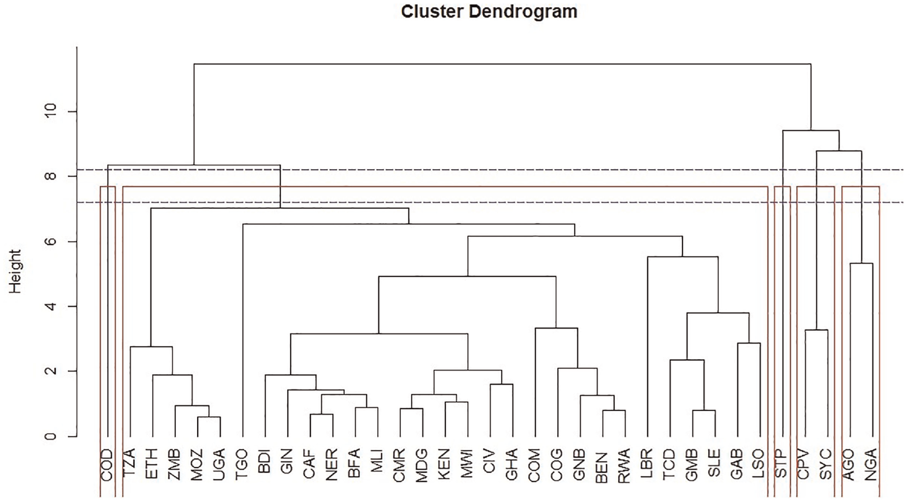
Cluster dendrogram – 2000.

From Figure 1, five cluster groupings can be observed between points 7.2 and 8.2 of the cophenetic distance/height (highlighted with the blue dotted line). These include, from the right-hand side, Nigeria (NGA) and Angola (AGO), Seychelles (SYC) and Cabo Verde (CPV), Sao Tome and Principe (STP) is an outlier, then Lesotho (LSO) to Tanzania (TZA) with Congo, Dem. Rep. (COD) also outlying. A good statistical technique to validate the clustering of cases is to compare the cophenetic distance with the original (unmodelled) data (Kassambara, 2017). To do this, a cophenetic correlation coefficient is applied. Here, the magnitude of this value should be close to 1 for a high-quality clustering solution (Saraçli et al., 2013). Usually, as a rule of thumb, values above 0.75 suggest good clustering. For the year 2000, the results showed a cophenetic correlation coefficient of 0.82, suggesting the clustering solution is a good fit.

Another common practice to validate the HCA outputs is by comparing how members of each cluster group compare with other members (within-cluster comparison), and with members within other (neighbouring) clusters. This can be done through a silhouette analysis (Wang et al., 2017). The silhouette coefficient measures the average dissimilarity between a case and the cases within the same cluster group, and the average dissimilarity of all cases outside the cluster group. If the silhouette width is close to 1, then the case shares strong similarities with its cluster members. If negative values are produced, then the case shows more similarities with cases within another cluster. For cases that have scores of around 0, these cases can be considered to be between the clusters (Engelbrecht, 2005). The silhouette analysis suggests that in 2000, Nigeria shared more similarities with members within the clustering of Lesotho (LSO) to Tanzania (TZA).

From these checks, one can start to qualitatively validate and evaluate the relationship between cases. For instance, in Angola and Nigeria, despite the silhouette analysis suggesting slightly more similarities (−0.05) between Nigeria and members within the clustering of Lesotho (LSO) to Tanzania (TZA), it is evident from qualitative knowledge that both countries are lower-middle income economies and leading oil exporters within the region. For this reason, they are more likely to share more similarities in economic indicators. Another interesting clustering is that of Cabo Verde and Seychelles, although these economies differ in terms of developmental levels (i.e. low income and lower-middle-income respectively), they are both island countries with relatively smaller economies. The same HCA process is applied to the dataset for the remaining time points (i.e. 2008 and 2015) and the output can be found in Supplemental Appendix C (summary in Table 1).

Table 1.

HCA output 2000–2015.

Year	Cluster	N	Cases
2000	Cluster A	2	AGO, NGA
	Cluster B	29	BEN, BFA, BDI, CMR, CAF, TCD, COM, COG, CIV, ETH, GAB, GMB, GHA, GIN, GNB, KEN, LSO, LBR, MDG, MWI, MLI, MOZ, NER, RWA, SLE, TZA, TGO, UGA, ZMB
	Cluster C	2	CPV, SYC
	Cluster D	1	COD
	Cluster E	1	STP
2008	Cluster F	3	AGO, BDI, LSO
	Cluster G	16	BEN, BFA, CMR, CAF, TCD, COM, CIV, GMB, GIN, GNB, KEN, MDG, MWI, MLI, SLE, TGO
	Cluster H	4	CPV, LBR, STP, SYC
	Cluster I	9	COD, ETH, GHA, MOZ, NER, RWA, TZA, UGA, ZMB
	Cluster J	3	COG, GAB, NGA
2015	Cluster K	9	AGO, COD, ETH, GHA, KEN, MWI, MOZ, NGA, TZA
	Cluster L	18	BEN, BFA, BDI, CMR, CAF, TCD, CIV, GAB, GMB, GIN, GNB, MDG, MLI, NER, RWA, TGO, UGA, ZMB
	Cluster M	6	CPV, COM, LSO, LBR, STP, SYC
	Cluster N	1	COG
	Cluster O	1	SLE

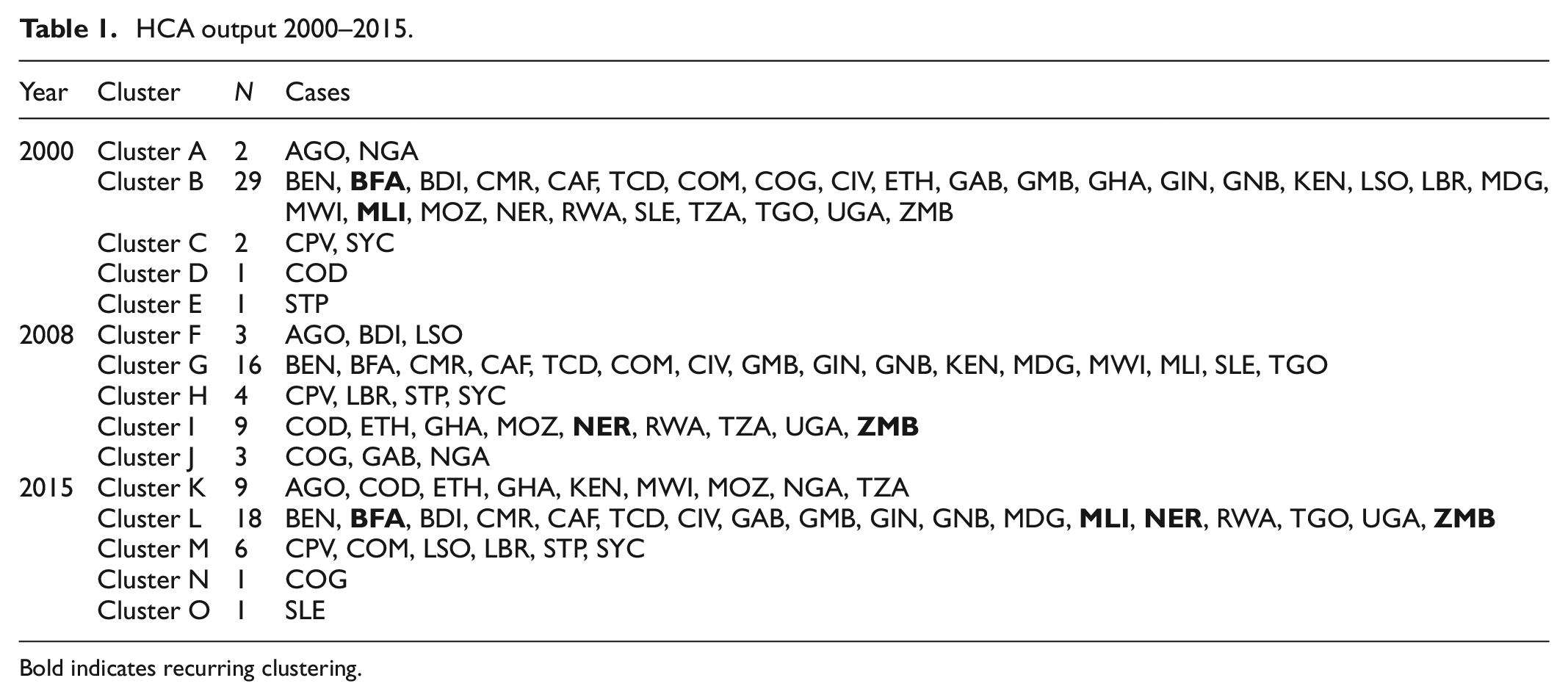
Bold indicates recurring clustering.

Similar to the clustering output for the year 2000, five cluster formations were also observed between points 7.2 and 8.2 of the cophenetic distance for 2008 (Supplemental Figure C2 – Supplemental Appendix C). However, for 2015 (Supplemental Figure C3 – Supplemental Appendix C), a higher cut off point was chosen (between 7.4 and 8.4) based on the HCA output. To validate the clustering, a cophenetic correlation coefficient of 0.76 and 0.7 was identified for 2008 and 2015, respectively. The silhouette analysis for the year 2008 showed that Burundi (Cluster F), Niger (Cluster I), Cabo Verde and Seychelles (both in Cluster H) shared similarities with Cluster G and Nigeria and Gabon (both in Cluster J) shared similarities with Clusters G and I respectively. For the period after the financial crisis (2015), Tanzania, Malawi, Mozambique, Congo, Dem. Rep., Kenya (all in Cluster K) and Comoros (Cluster M) were seen to share similarities with members of Cluster L. The silhouette output can be found in Supplemental Appendix F. All cases with negative values would be discussed in the configurational model.

When placed alongside each other, HCA dendrograms can also be used to compare the similarities in case clustering across two time points. This can be done by measuring the level of entanglement (Kassambara, 2017). That is to say, the quality of alignment between case cluster groups across two dendrograms. An entanglement distance can be used to assess the extent of growth in similarities across cases over time (i.e. sigma-convergence). In this sense, the entanglement measure serves as a dispersion index (Heinze and Knill, 2008) – demonstrating the level of similarity and differences over time. Statistically, entanglement is measured between 1 (full entanglement) and 0 (no entanglement). A lower entanglement coefficient represents good alignments (Kassambara, 2017).

The entanglement for the period before the financial crisis (2000/2008) was 0.47 with no re-emerging case pairing (Supplemental Figure C4). This suggests a decrease in similarities between the start of the MDGs and the 2008 financial crisis – a higher entanglement coefficient represents lesser similarities across cluster groupings. The observation of lesser similarities across this time point highlights the varying impacts the financial crisis had on each economy. For the period after the financial crisis (2008/2015), economies within the Sub-Saharan region begin to share more macroeconomic similarities as compared to the period before the crisis. This is reflected in the lower entanglement coefficient score of 0.37. During this time interval (2008/2015) the clustering of Zambia and Niger re-emerges (Supplemental Figure C5). Lastly, for the duration of the MDGs (i.e. 2000/2015) an entanglement of 0.43 was detected with Mali (MLI) and Burkina Faso (BFA) as the re-emerging cluster pairs (Supplemental Figure C6). Indicating dissimilarities between the convergence situation at the start and end of the MDGs.

Fluctuations in the entanglement values and re-emerging cases also indicate a high degree of macroeconomic complexity in the political economy of the Sub-Saharan Africa region. Evidently, the impact of the 2008 financial crisis is seen to have affected the growth in macroeconomic similarities within the region. Having observed longitudinal case patterns in the HCA, it is also possible to assess variables influencing case clustering using inferential and descriptive statistics. This is useful in situations when a researcher seeks to produce generalisable findings. However, in more detailed comparative case studies, an in-depth case comparison and further cluster validation can be achieved through the use of configurational modelling. Configurational tables allow for understanding the variations in variable patterns across case and cluster configurations. This provides a comparison of specific variable influences on within-case clustering and cross-cluster comparison.

Configurational model

To explore patterns in variable trends, especially those influencing case clustering, a combination of correlation coefficients and correlation tests are first applied to observe the direction of movement between variables (Emerson et al., 2012). The output for the three time points can be found in Supplemental Appendix E. From this, a positive significant correlation between general government revenue (GGR) and general government total expenditure (GGE) is noticed. This was especially significant during (2008) and after (2015) the financial crisis. This indicates that, at those time points (2008/2015), these two variables operated in tandem – in instances where one increased or reduced, it is likely similar impacts were experienced by the other. For the outcome variable (FDI), there was no significant correlation with the other variables.

For the configurational model, the same scaled HCA dataset is used to observe variable interactions across case clustering over the period under discussion. Configurational modelling seeks to identify patterns resulting in the formation of clusters, and how each cluster compares with another. This approach stresses an understanding of the features of each cluster group, allowing for within and cross-cluster comparison and validation of case configurations in the HCA output. Here, data is coded through a process of calibration – that is, transforming data into set membership scores. This is achieved using either binary ‘crisp’ coding where variables (attributes) are coded into scores of ‘0’ to indicate below a threshold and ‘1’ to indicate above a threshold. Or, ‘fuzzy’ values over a continuous range between ‘0’ and ‘1’. Thresholds should be theoretically conceptual based on the empirical knowledge of cases.

In this example application, the standardised dataset is presented in the configurational modelling such that individual case scores are considered with regard to their point on the central tendency of each variable distribution, either being above threshold, or below threshold. The central tendency point used is the mean. The output for each time period can be found in Supplemental Appendix D. Colour scales illustrate trends in the scaled data, green indicates higher values (i.e. above the variable central tendency) while red suggests lower values (i.e. below the variable central tendency). At this stage of the analysis IMF intervention indicators are added to reflect the total number of interventions each country experienced between the period before (2000/2007) and after (2008/2015) the financial crisis (see Supplemental Table D2 and D3 in Appendix D). This approach to configurational modelling allows the researcher to observe diversity in the scaled variable scores.

With some datasets, observing average variable trends across cluster groups can be useful in painting an overall picture (see Table 2). This can aid in the development of a typology or hierarchy of cluster grouping based on the performance in an outcome variable (in this case FDI), and in singling out variables influencing outliers – for instance in 2000 Cluster D has the highest IACP% and lowest GDP, GGE and GGR; and interesting cases – in the same year Cluster A consists of oil exporters and highest average cluster FDI scores. In longitudinal comparative analysis, Table 2 can also be used to observe variables influencing the movement of cases over time. For instance, combined, members of Cluster A had the highest average FDI and FDI% scores (and the lowest NBTT) for 2000. In 2008, Angola is paired with Lesotho and Burundi (Cluster F) while Nigeria is grouped within Cluster J (Congo, Rep. and Gabon). For that year, combined, members of Cluster J had the highest average scores for FDI, GGNLB and NBTT; and the lowest average cluster scores for GDP%. For Cluster F, combined, members had scores lower than the average FDI, the lowest scores for FDI% and the highest average cluster scores for GDP%, GGR and GGE. Suggesting that between 2000 and 2008, Nigeria had more FDI inflows as compared to Angola. The observation of longitudinal patterns across case clustering over time can aid in providing a summary picture of patterns in variable and case movement.

Table 2.

Configurational model – average variable trends per cluster (2000–2015).

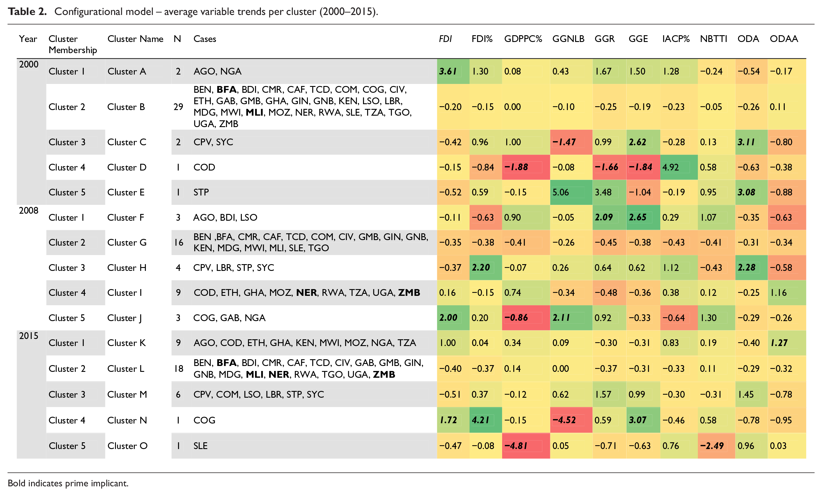
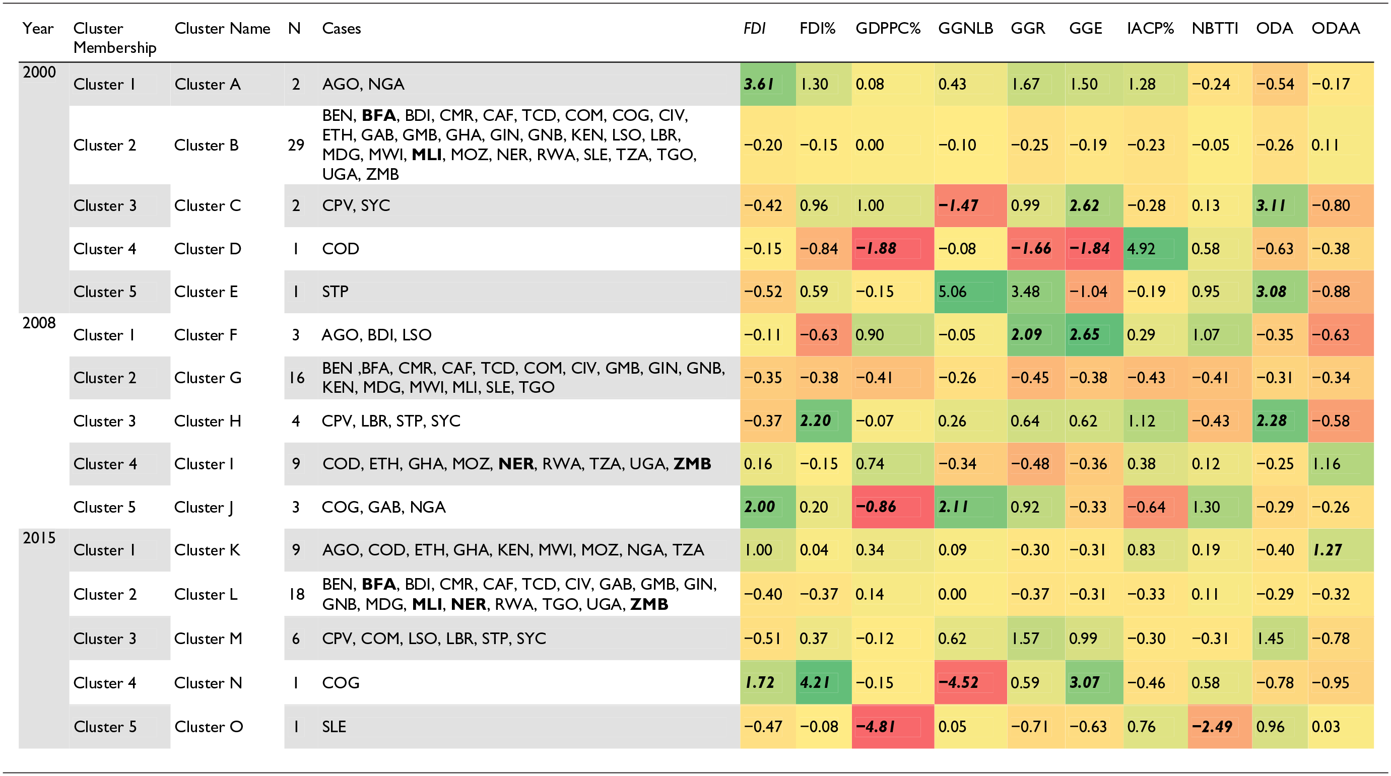
Bold indicates prime implicant.

The configurational model for each time point (Supplemental Table D1, D2 and D3 in Appendix D) can also be used in validating cases with negative scores produced during the silhouette analysis (i.e. Nigeria in 2000; Burundi, Niger, Cabo Verde, Seychelles, Nigeria and Gabon in 2008; and Tanzania, Malawi, Mozambique, Congo, Dem. Rep., Kenya and Comoros in 2015). Here, the researcher is able to identify variable patterns that may make a case more fitting for its proposed cluster (or neighbour). At this stage, the researcher can also observe mathematical ‘near misses’ in the data that may indicate some degree of similarity. That is to say, instances where cases within a cluster share similar above (or below) threshold scores for a specific variable but one or two cluster members have a score slightly below (or above) or relatively close to the threshold. In the example dataset, Cluster L (Supplemental Table D3) provides an illustration of a near miss. In this cluster, most members seem to share scores below the central tendency for FDI%, with exception of Niger and Zambia. Yet, Niger and Zambia have values of 0.05 and 0.06, respectively. These values are close to the threshold (0.00), and the value for Togo (−0.05).

The silhouette analysis for the first time point (2000) suggested Nigeria (−0.05) shared slightly more similarities to members in Cluster B as compared to Cluster A. From the configurational model (Supplemental Table D1), it becomes evident that although Nigeria had comparatively lower scores for GGR, GGE and IACP% members of Cluster A share strong similarities in their FDI inflows. That year Nigeria and Angola had the highest FDI inflows. Members of Cluster B also share more similarities in IACP% – all with values below the central tendency. For the year 2008, the silhouette analysis suggests Burundi (Cluster F), Niger (Cluster I), Cabo Verde and Seychelles (both in Cluster H) shared similarities with members of Cluster G and Nigeria and Gabon (both in Cluster J) also shared similarities with Clusters G and I respectively. The configurational model for that year shows that most cases in Cluster G have values below the central tendency for FDI, GGNLB, GGR, NBTT and ODA. Evidently, the comparatively higher values in GGR and GGE for Burundi make it more similar to members within Cluster F. Niger is also seen to have more similarities with members of Cluster I as compared to Cluster G. This is evident in the above threshold score for GDP%. For Cabo Verde and Seychelles, both cases are also seen to have scores above the central tendency for FDI%, GGR, GGE and ODA making them more similar to Cluster H as compared to Cluster G. Nigeria and Gabon also have scores above the threshold for FDI, GGNLB and NBTT – making them more similar to Cluster J then the suggested clusters.

For the period after the financial crisis (2015), Tanzania, Malawi, Mozambique, Congo, Dem. Rep. and Kenya (all in Cluster K) and Comoros (Cluster M) were all seen to share similarities with members of Cluster L. Cases within Cluster L share similarities in below threshold scores for FDI (i.e. except Zambia), FDI% (i.e. except. Zambia and Niger) and ODAA (i.e. except Burkina Faso, Mali and Uganda). Conversely, cases within Cluster K have comparatively higher ODAA scores and Comoros has higher values for GGNLB and GGR, making these cases more similar to members of Cluster M. In this example dataset, majority of the negative values suggested in the silhouette analysis remain close to 0. This indicates that these cases could remain in their current cluster group or moved to another similar cluster. For this reason, the HCA outputs for each time point is retained. In this sense, the configurational model is used to validate the clustering of cases by searching for possible patterns in the data that reaffirm (or otherwise) cluster membership, especially for cases with negative values produced in the silhouette analysis.

The identification of patterns in the data also enables the researcher to compare cases within, and across, cluster grouping. From this synthesis, patterns begin to appear. A text summary ‘Cluster Profile’ can also be produced for each time point summarising variable patterns observed in the data (see Supplemental Appendix G Tables G1, G2 and G3). An additional column can be added to include important variable patterns for individual cases for cross-case comparison and observing trajectories. It is important to note that, throughout this synthesis of variable and case movement over time, the researchers detailed qualitative knowledge of cases becomes essential in understanding the configurations. Additional applied statistical approaches can also be used to produce more statistically generalisable information (see for instance Haynes, 2014).

Assessing IMF impacts on FDI during the MDGs

Having affirmed the structure of each cluster, and identified convergent patterns in the data, one can proceed to consider the possible impacts of IMF interventions on FDI inflows. At this stage, IMF intervention variables are added to the data. To highlight longitudinal trends in the dataset, the configurational model is recoded to place emphasis on cases that experience variable trends consistently above or below the threshold throughout the period under analysis – see Supplemental Appendix I. For cases that have inconsistent variable trends, this is left blank.

When assessing IMF impacts, the researcher starts by observing the macroeconomic situation at the first time point (i.e. 2000 – in this case the baseline assessment or the start of the MDGs). In the year 2000, the HCA output produced five clusters, two cases were outliers (Supplemental Figure C1 in Appendix C). While remaining heterogenous, cases within each cluster share some similarities in one or more variables based on how they compare to the average performer that year (Supplemental Table D1 in Appendix D). From this starting point, an assessment of IMF interventions impacting changes in FDI inflows over time is conducted. During the period before the financial crisis, a total of fifty-eight IMF interventions had been implemented across 30 (out of 35) cases (Supplemental Table D2). From Supplemental Table D2 (Supplemental Appendix D – highlights variable trends for cases in 2008) and Supplemental Table I1 (Supplemental Appendix I highlights consistency in below and above variable threshold scores for cases between 2000 and 2008), it is evident that there is no pattern/configuration in the data suggesting a number of IMF interventions impacting the clustering of cases – or FDI. By 2008, cases that experienced one IMF intervention show varying impacts on FDI (although sharing similarities in above threshold scores for NBTT). For cases that have FDI values above the central tendency, they also share similar above threshold values for FDI%. The same is observed for cases with below threshold scores for FDI – similar FDI% values below the central tendency.

In the same year (2008), with exception of Madagascar and Nigeria, cases that experienced two IMF interventions shared FDI scores below the central tendency. Madagascar and Nigeria also shared similar above threshold scores for GDP% and ODAA, and similar below threshold scores for GGR, GGE, IACP% and ODA. Both countries also belong to different cluster formations. For cases that experienced three IMF interventions, only Cameroon had values below the central tendency for FDI inflows. These cases also share similarities in below central tendency scores for FDI%, GGE and IACP%. Rwanda and Uganda both experienced the highest number of interventions between 2000/2007 (four each). Both cases had different levels of FDI inflows but share similar above threshold scores for GDP% and ODAA, and similar below threshold scores for FDI%.

For the period after the financial crisis (Supplemental Table D3), a decrease in the total number of IMF interventions experienced across the region can be observed. This is as compared to the previous time interval – from 59 interventions between 2000 and 2007 to 49 interventions between 2008 and 2014. By 2015, cases with no IMF interventions between 2008 and 2014 had values below the central tendency for FDI – with exception of Nigeria. These cases also share similar negative values for GGR, GGE and ODA – although across these cases Nigeria’s values are comparatively higher. Out of the 18 cases that experienced one IMF intervention, Angola had very high values for FDI (the highest that year), Ghana and Congo, Rep. also had comparatively higher FDI values and Ethiopia and Congo, Dem. Rep had scores slightly above the central tendency. The remaining cases have FDI scores below the average. For cases that experienced two IMF interventions between 2008/2015, only Mozambique had scores above threshold for FDI, the remaining cases having below threshold values. This pattern is similar to cases that implemented three interventions – with only Tanzania demonstrating FDI scores above the central tendency.

From the observation of IMF interventions impacts prior to, and after, the financial crisis, complex causal configurations become evident in relation to FDI inflows, and convergent patterns. In some cases, IMF interventions are seen to have impacts (e.g. Nigeria, Ghana and Congo., Rep between 2000/2008), in others impacts are not evident. At this stage, one can begin to synthesise the DPS output. To highlight a few trends, in the cluster with the highest average cluster FDI values for 2000 (Cluster A), Nigeria (second highest FDI that year) is seen to share similarities with Angola, between 2000/2008, Nigeria implemented two IMF interventions and had the highest FDI inflows in 2008 (Cluster J). Angola had the highest FDI inflows in 2000, did not implement an IMF intervention between 2000/2008, and had a drop in FDI inflows in 2008 (Cluster F). Interestingly, by 2015 Angola and Nigeria cluster together (Cluster K) with Angola having the highest FDI inflows that year while Nigeria had comparatively lower values for FDI. Angola experienced one IMF intervention and Nigeria did not experience an IMF intervention during that interval.

Similar patterns are seen when observing cases that experienced lower FDI inflows in 2000 (below −0.50), that is Congo, Rep., Benin, Comoros, Guinea-Bissau, Central African Rep. (all within Cluster B) and Sao Tome and Principe (Cluster E). Variations in cluster formations for subsequent time points highlight varying impacts of the financial crisis and IMF interventions. In 2008, Central African Rep., Benin, Guinea-Bissau and Comoros remained clustered together (Cluster G – low FDI, FDI%, GGR and ODA). Across the 2000/2008 period, these economies also implemented varying IMF interventions. By 2015, Benin, Central African Rep. and Guinea-Bissau remain together in Cluster L (low FDI and FDI%) while Comoros moves to Cluster M (Low FDI and ODAA; High GGR and GGE) and Sao Tome and Principe (an outlier in 2000) start to share similarities with members of Cluster H in 2008. With exception of Sao Tome and Principe (experienced two IMF interventions), Benin, Central African Rep., Guinea-Bissau and Comoros all implemented an IMF intervention each. These observations suggest equifinality in achieving higher FDI inflows (i.e. similar FDI outcomes resulting from varying numbers of IMF interventions). At the same time, it is evident that cases with similar starting points also end up with different FDI inflows (i.e. multifinality).

In longitudinal applications, the researcher can observe trends in the data to highlight variables influencing ‘convergent’ cases. That is to say, cases that remained closely clustered together over two time points. In the example application, the HCA output comparing the period after the financial crisis (2008/2015) showed that Zambia and Niger shared strong similarities (converged) during that time interval. From the configurational model (Supplemental Table D2 and D3), it becomes evident that, across these time points, while both cases demonstrate differences in FDI inflows (Zambia experiencing comparative more inflows than Niger), these cases possess some similarities in threshold scores for FDI%, GDP%, GGE and NBTT. For Mali and Burkina Faso (converged between 2000/2015), both cases demonstrate similarities in threshold scores for FDI, FDI%, GDP%, GNLB, GGR and IACP% across the two time points.

Discussion

Our analysis examines the convergence trends in Sub-Saharan Africa during the Millennium Development Goals in the context of sigma and delta convergence. Sigma-convergence indicates that nations are showing increasingly similar macroeconomic outcomes, suggesting growing homogeneity. Delta-convergence assesses how countries’ economic policies align with ideal outcomes such as increased FDI, often influenced by IMF strategies.

For sigma convergence, our data shows a modest improvement over time in the consistency of cluster formations, as evidenced by the Adjusted Rand Index (ARI), which rose from 0.21 in 2000 versus 2008 to 0.24 in 2008 versus 2015. However, Dendrogram Correlation and Silhouette Scores indicate a decrease in cluster stability and cohesion over time, suggesting that the quality of clustering has diminished, likely due to evolving economic policies or external factors. Interestingly, while the ARI suggests a slight improvement in clustering consistency, other metrics like Silhouette and Entanglement Scores reveal a decrease in cluster quality and distinctiveness. This discrepancy highlights the complex dynamics at play, which include shifts in economic policies and external economic shocks that might have influenced these trends.

In our delta-convergence analysis, the impact of IMF interventions on economic indicators like FDI does not show a consistent pattern. While some countries with frequent IMF engagements, like Rwanda (6) and Ghana (2), have seen certain economic improvements, the overall effect on FDI is mixed. For example, Ghana shows positive trends potentially due to successful IMF-supported reforms, while others like Tanzania and Uganda display less consistent FDI outcomes. The effectiveness of IMF interventions varies significantly with each country’s specific situation and responsiveness. Rwanda and Uganda, despite similar levels of IMF interactions, show varying outcomes in fiscal measures such as General Government Revenue and Net Lending/Borrowing. This variability underscores the nuanced impact of IMF policies, suggesting that alignment with IMF recommendations might enhance macroeconomic stability and attract more FDI, though this is not universally the case across all countries studied. This analysis demonstrates that while IMF interventions may influence global economic policies, their direct impact on enhancing FDI in Sub-Saharan Africa during the specified period has been mixed, reflecting a complex interplay of local and international interactions.

Conclusion

This paper demonstrates an example application of DPS in assessing the macroeconomic convergence situation for Sub-Saharan African economies that implemented IMF interventions between the years 2000 and 2015. DPS method enables longitudinal applications, offering the possibility of examining the stability (or instability) of variable scores by observing changes in variable trends over time. In this research, DPS assessed stability and instability within countries during the period before and after the financial crisis, with a focus on stability in variable threshold scores for FDI and other key macroeconomic indicators.

Reflecting on the findings from the DPS analysis, it becomes evident that the method not only captures the nuances of socio-economic and political groupings but also reinforces the validity of DPS as a robust tool for macroeconomic analysis. The DPS also provides a structured systematic analysis that not only confirms the groupings of cases but also enhances them with robust empirical evidence. Such detailed insights are crucial for shaping informed policy decisions and advancing academic research within the Sub-Saharan African context. Moreover, additional qualitative data could be added to the model to test for additional patterns. A central point of this research was the impact of exogenous shocks on economic stability, specifically, the impact of IMF interventions on macroeconomic indicators. Considering this, the DPS method can be modelled in a way that permits the addition of variables that assist in assessing exogenous economic and policy interventions within and across groups of cases, taking into consideration the specific context in which an intervention was implemented.

DPS also assists in inferring causation as it allows for considerations of ‘complex causal configurations’ and provides the researcher with the possibility of capturing ‘complex paradoxicality’ across sample cases. This is evident when an outcome variable is added to the model to test for dynamics and stability. In the example application, it is observed that IMF interventions do not necessarily have significant effects on FDI convergent patterns. This is based on the varying causal mechanisms triggering the convergent changes across cases and the facilitating factors that affect the effectiveness of these mechanisms. Suggesting the presence of ‘multiple conjunctural causation’ across cases, causation that is not necessarily permanent and subject to different circumstances which may result in the same or different outcomes. This was reflected in the configurational results which show disparities in variables that bind convergent cases and cluster groups together.

In the example application, the DPS method highlights the importance of individual country differences and suggests that there are multiple paths to a given policy outcome (FDI), rather than a single optimal economic strategy. This raises policy issues associated with economic complexity, such as how best to create an overall environment of stability that might promote convergence and reduce instability. DPS benefits significantly from R’s robust computational power, particularly when managing large datasets. R enhances DPS by allowing detailed analysis through clear visualisations and effective data handling, especially useful in cases of dense dendrograms. This facilitates focussed investigations into specific data groupings and improves the accuracy of cluster analysis. Moreover, R supports the comparison of average cluster variable patterns, simplifying the classification of extensive groups and enhancing the analytical depth. These capabilities are crucial for applying DPS to larger and more complex datasets.

DPS’s structured approach to clustering and configurational analysis can enrich machine learning algorithms by providing an initial, interpretable grouping of data, which can be further explored using predictive or classification models. Similarly, in network models, DPS can help identify nodes or clusters with significant shared attributes, facilitating a more nuanced understanding of network dynamics. Advancing DPS’s scalability could involve integrating more sophisticated computational methods and parallel processing techniques. This enhancement would broaden DPS’s applicability in macroeconomic research and other areas dealing with large, complex datasets, pushing the boundaries of what can be achieved with this analytical approach. There is significant potential to expand the application of DPS to other regions and different types of economic data. Future studies could explore the application of DPS in analysing economic patterns in regions beyond Sub-Saharan Africa, such as in emerging Asian or Latin American markets. Utilising DPS to examine diverse economic indicators—such as digital economy metrics or sustainability indices—could offer new insights and validate the method’s effectiveness across different economic contexts. These expansions not only broaden the applicability of DPS but also contribute to a more detailed and nuanced global economic analysis.

Supplemental Material

sj-doc-1-mio-10.1177_20597991241256791 – Supplemental material for Systems dynamics and causal configurations: Using dynamic pattern synthesis for macroeconomic comparative research

Supplemental material, sj-doc-1-mio-10.1177_20597991241256791 for Systems dynamics and causal configurations: Using dynamic pattern synthesis for macroeconomic comparative research by David Alemna and Philip Haynes in Methodological Innovations

Footnotes

Acknowledgements

This research was also supported by funding from the University of Portsmouth through UKRI grants, enabling open access publication.

Correction (October 2024):

Article updated to add Acknowledgements section.

Declaration of conflicting interests

The author(s) declared no potential conflicts of interest with respect to the research, authorship, and/or publication of this article.

Funding

The author(s) disclosed receipt of the following financial support for the research, authorship, and/or publication of this article: This research was partly conduct under an Economic and Social Research Council research grant aimed at providing empirical applications of innovative quantitative methodologies [Project Reference: ES/W005743/1]. Aspects of this paper was submitted to the NAEC New Analytical Tools and Techniques for Economic Policymaking Conference 2019. OECD, New Approaches to Economic Challenges, France.

ORCID iD

David Alemna

Supplemental material

Supplemental material for this article is available online. The re-coded dataset and R script is available in RDA format from the corresponding author on reasonable request.

Author biographies

David Alemna is teaching fellow at the University of Portsmouth and a Consultant at ICF - Inner City Fund (UK). He previously served as an ESRC South Coast Doctoral Training Partnership Post Doc Fellow at the University of Portsmouth. He completed is PhD research on comparative public policy and policy transfer, using configurative methods in 2020, and has also worked on policy research for an international consultancy.

Philip Haynes is Professor of Public Policy at the University of Brighton. His research includes the use and development of methods that better represent the complexity of social and economic policy systems.

References

Aldenderfer

Blashfield

(1984) Cluster Analysis: Quantitative Applications in the Social Sciences. Beverly Hills: Sage.

Anderberg

(1973) Cluster Analysis for Applications: Probability and Mathematical Statistics: A Series of Monographs and Textbooks (Vol. 19). Academic Press.

Arthur

(2013) Complexity Economics. Oxford: Oxford University Press.

Barbrook-Johnson

Schimpf

Castellani

(2019) Reflections on the use of complexity-appropriate computational modeling for public policy evaluation in the UK. Journal on Policy and Complex Systems 5(1): 55–70.

Berg-Schlosser

De Meur

Rihoux

, et al. (2009) Qualitative comparative analysis (QCA) as an approach. In: Rihoux

Ragin

(eds) Configurational Comparative Methods: Qualitative Comparative Analysis (QCA) and Related Techniques, vol. 1, p.18.

Bicket

Christie

Gilbert

, et al. (2020) Handling Complexity in Policy Evaluation: Supplementary Gude to Magenta Book. London: HM Treasury.

Bicket

Hills

Wilkinson

, et al. (2021). Don’t panic: Bringing complexity thinking to UK Government evaluation guidance. Evaluation 27(1): 18–31.

Bryman

(2008) The End of the Paradigm Wars. The SAGE Handbook of Social Research Methods. Thousand Oaks, CA: Sage, pp.13–25.

Bleiklie

(2001). Towards European convergence of higher education policy. Higher Education Management 13(3).

10.

Burch

Heinrich

(2015) Mixed Methods for Policy Research and Program Evaluation. Thousand Oaks, CA: Sage.

11.

Burns

(2007) Systemic Action Research: A Strategy for Whole System Change. Bristol: Policy Press.

12.

Byrne

(2002) Interpreting Quantitative Data. Thousand Oaks, CA: Sage.

13.

Cairney

(2012) Complexity theory in political science and public policy. Political Studies Review 10(3): 346–358.

14.

Creswell

Clark

VLP

(2017) Designing and Conducting Mixed Methods Research. Thousand Oaks, CA: Sage.

15.

Emerson

Green

Schloerke

, et al. (2012). The generalized pairs plot. Journal of Computational and Graphical Statistics 22(1): 79–91.

16.

Engelbrecht

(2005) Fundamentals of Computational Swarm Intelligence. Chichester: John Wiley & Sons.

17.

Fletcher

(2017) Applying critical realism in qualitative research: Methodology meets method. International Journal of Social Research Methodology 20(2): 181–194.

18.

Glattfelder

(2013) Decoding Complexity: Uncovering Patterns in Economic Networks. Heidelberg: Springer.

19.

Greene

Caracelli

Graham

(1989) Toward a conceptual framework for mixed-method evaluation designs. Educational Evaluation and Policy Analysis 11(3): 255–274.

20.

Hair

Black

Babin

, et al. (1998) Multivariate Data Analysis, vol. 5, pp.207–219. Upper Saddle River: Prentice Hall.

21.

Hakura

Nsouli

MSM

(2003) The Millennium Development Goals, Capacity Building, and the Role of the IMF. Washington: International Monetary Fund.

22.

Haynes

(2014) Combining the strengths of qualitative comparative analysis with cluster analysis for comparative public policy research: With reference to the policy of economic convergence in the euro currency area. International Journal of Public Administration 37(9): 581–590.

23.

Haynes

Alemna

(2022) From aggregations to multimethod case configurations. Case diversity in quantitative analysis when explaining COVID-19 fatalities. International Journal of Social Research Methodology 27(2): 147–158.

24.

Haynes

Alemna

(2023a) Convergence trends in Euro Economies: Financial crisis recovery and the COVID-19 pandemic. Economies, 11(11), 284. https://doi.org/10.3390/economies11110284

25.

Haynes

Alemna

(2023b) Dynamic Pattern Synthesis Chichester: White Horse Books. Available at: https://whb.co.uk/new-publication-on-dynamic-pattern-synthesis-2023/

26.

Haynes

(2017) Social Synthesis: Finding Dynamic Patterns in Complex Social Systems. London: Routledge.

27.

Haynes

(2016) Convergence and heterogeneity in Euro based economies: Stability and dynamics. Economies 4(3): 16.

28.

Heichel

Pape

Sommerer

(2005) Is there convergence in convergence research? an overview of empirical studies on policy convergence. Journal of European Public Policy 12(5): 817–840.

29.

Heinze

Knill

(2008) Analysing the differential impact of the Bologna Process: Theoretical considerations on national conditions for international policy convergence. High Educ 56: 493–510.

30.

Hodgson

(2014) Economics in the Shadows of Darwin and Marx. Cheltenham: Edward Elgar Publishing.

31.

IMF (2001) IMF managing director’s report to the International Monetary and Financial Committee Streamlining Conditionality and Enhancing Ownership. IMF. Available at: https://www.imf.org/external/np/omd/2001/110601.htm (accessed 20 October 2018).

32.

Inman

(2019, ). Georgieva’s brave new agenda at IMF threatened by economic storm clouds. The Guardian, 29 November, 2019. Available at: https://www.theguardian.com/business/2019/oct/12/kristalina-georgieva-imf-washington-climate-crisis

33.

Jessop

Knio

(eds.) (2018) The Pedagogy of Economic, Political and Social Crises: Dynamics, Construals and Lessons. London: Routledge.

34.

Johnson

Onwuegbuzie

(2004) Mixed methods research: A research paradigm whose time has come. Educational Researcher 33(7): 14–26.

35.

Kassambara

(2017) Practical Guide to Cluster Analysis in R: Unsupervised Machine Learning, vol. 1. STHDA. Available at: clustering_english_edition1_amazon(datanovia.com)

36.

Kaufman

Rousseeuw

(2009) Finding Groups in Data: An Introduction to Cluster Analysis, vol. 344. New York, NY: John Wiley & Sons.

37.

Knill

(2005) Introduction: Cross-national policy convergence: Concepts, approaches and explanatory factors. Journal of European Public Policy 12(5): 764–774.

38.

Morçöl

(2013) A Complexity Theory for Public Policy. London: Routledge.

39.

Pawson

Tilley

(1997) Realistic Evaluation. Sage.

40.

Pawson

Tilley

(2001) Realistic evaluation bloodlines. American Journal of Evaluation 22(3): 317–324.

41.

Radelet

(2004) Aid effectiveness and the millennium development goals. Center for Global Development Working Paper (39). Center for Global Development. Washington. Available at: https://ssrn.com/abstract=1112641 or http://dx.doi.org/10.2139/ssrn.1112641

42.

Ragin

(1987) The Comparative Method: Moving Beyond Qualitative and Quantitative Methods. Berkeley, CA: University of California.

43.

Ragin

(1997) Turning the tables: How case-oriented methods challenge variable-oriented methods. Comparative Social Research 16(1): 27–42.

44.

Rodrik

(2003) Challenges to the World Bank and IMF: Developing country perspectives. London: Anthem Press.

45.

Rokach

Maimon

(2005) Clustering methods. In Maimon

Rokach

(eds) Data Mining and Knowledge Discovery Handbook. Boston, MA: Springer, pp.321–352.

46.

Romesburg

(2004) Cluster Analysis for Researchers. Morrisville: Lulu Press.

47.

Saraçli

Doğan

(2013) Comparison of hierarchical cluster analysis methods by cophenetic correlation. Journal of inequalities and Applications 2013(1): 1–8.

48.

Schimpf

Barbrook-Johnson

Castellani

(2021) Cased-based modelling and scenario simulation for ex-post evaluation. Evaluation 27(1): 116–137.

49.

Schimpf

Castellani

(2020) COMPLEX-IT: A case-based modelling and scenario simulation platform for social inquiry. Journal of Open Research Software 8(1): 25.

50.

Shorten

Smith

(2017) Mixed methods research: Expanding the evidence base. Evidence-Based Nursing 20(3): 74–75.

51.

Schneider

Wageman

(2010) Standards of good practice in qualitative comparative analysis (QCA) and fuzzy sets. Comparative Sociology 9(3): 397–418.

52.

Taylor

Haynes

Darking

(2020). English local government finance in transition: Towards the marketization of income. Public Management Review 23(7): 1081–1106.

53.

Tilley

Pawson

(2000) Realistic evaluation: An overview. In Founding Conference of the Danish Evaluation Society, vol. 8.

54.

Wang

Franco-Penya

Kelleher

, et al. (2017) An analysis of the application of simplified silhouette to the evaluation of k-means clustering validity. In: International Conference on Machine Learning and Data Mining in Pattern Recognition, 15–20 July, 2017, New York. Cham: Springer, pp.291–305.

55.

Wilks

(2011) Cluster Analysis. In International Geophysics, vol. 100. Cambridge, MA: Academic Press, pp.603–616.

56.

Zachariadis

Scott

Barrett

(2013) Methodological implications of critical realism for mixed-methods research. MIS Quarterly 37: 855–879.

57.

Zelli

Gerrits

Möller

(2021) Global governance in complex times: Exploring new concepts and theories on institutional complexity. Complexity, Governance & Networks 6(1): 1–13.

Supplementary Material

Please find the following supplemental material available below.

For Open Access articles published under a Creative Commons License, all supplemental material carries the same license as the article it is associated with.

For non-Open Access articles published, all supplemental material carries a non-exclusive license, and permission requests for re-use of supplemental material or any part of supplemental material shall be sent directly to the copyright owner as specified in the copyright notice associated with the article.

0.00 MB

2.29 MB