Data Imbalances in Coincidence Analysis: A Simulation Study

Abstract

In this paper, we investigate the conditions under which data imbalances, a common data characteristic that occurs when factor values are unevenly distributed, are problematic for the performance of Coincidence Analysis (CNA). We further examine how such imbalances relate to fragmentation and noise in data. We show that even extreme data imbalances, when not combined with fragmentation or noise, do not negatively affect CNA’s performance. However, an extended series of simulation experiments on fuzzy-set data reveals that, when mixed with fragmentation or noise, data imbalances may substantially impair CNA’s performance. Furthermore, we find that the performance impairment is higher when endogenous factors are imbalanced than when exogenous factors are concerned. Our results allow us to quantify these impacts and demarcate degrees at which data imbalances should be considered as problematic. Thus, applied researchers can use our demarcation guidelines to enhance the validity of their studies.

Introduction

Coincidence Analysis (CNA; Baumgartner and Ambühl, 2020) is a novel method of causal learning that belongs to the family of configurational comparative methods (CCMs; Rihoux and Ragin, 2009). Unlike most methods of data analysis, CNA can handle complex causal structures involving conjunctivity (when multiple factors interact to produce an outcome) and disjunctivity (when alternative pathways produce the same outcome independently of one another), which do not necessarily exhibit pairwise dependencies between a cause and its effect. CNA accomplishes this by fitting complex Boolean functions as a whole to the data, and it is the only method of its kind capable of detecting links between multiple outcomes (sequentiality), which are characteristic for causal chains.

As such, CNA has been increasingly applied in a wide range of fields, including political science (e.g., Haesebrouck, 2023), environmental studies (e.g., Edianto, Trencher, and Matsubae, 2022), public health (e.g., Yakovchenko et al., 2020), medical informatics (e.g., Womack et al., 2022), sociology (e.g., Epple and Schief, 2016), and organizational behavior (e.g., Swiatczak, 2021). In parallel, methodological research has substantially improved the quality of CNA’s data analysis approach (e.g., Parkkinen and Baumgartner, 2023). However, data distribution requirements have not yet been investigated for CNA. This is all the more striking as, for example, within the framework of statistical methods, assessing data distributions is a crucial pre-analytical step for selecting appropriate methods and determining the expected accuracy of analyses. Accordingly, various data distribution characteristics have been widely shown to create issues for these methods (e.g., von Hippel, 2013; Yuan, Bentler, and Zhang, 2005).

This study examines how the performance of CNA is affected by a common data distribution characteristic: data imbalances (also referred to as skewness), which occur if factors have value distributions that partition the cases in the data into sets of notably unequal sizes. Such imbalances are often encountered in CCM applications. For instance, the vast majority of countries are classified as not wealthy based on the world bank GDP classification system (Goertz, 2020), decisions against the termination of pregnancy after a prenatal diagnosis of Down syndrome are very rare (Britt et al., 2000), educational poverty is a marginal occurrence in developed countries (Glaesser, 2022), and employees prevailingly consider themselves competent (Swiatczak, 2021).

Skewness has received some attention in the methodological literature on Qualitative Comparative Analysis (QCA; Ragin, 2009), another method from the family of CCMs (e.g., Oana, Schneider, and Thomann, 2021; Schneider and Wagemann, 2012). However, on the one hand, those discussions have so far focused on particular data examples, which do not yield quantitative performance assessments or generalizable conclusions. On the other hand, findings on QCA cannot be transferred to CNA because of substantive algorithmic differences between the two methods (Swiatczak, 2022). As a consequence, thus far, applied CNA researchers lack a means to determine whether their data are imbalanced to such an extent that countermeasures should be taken or reliable results can be expected.

The aim of this study is to remedy this situation by systematically investigating to what extent data imbalances affect the quality of CNA’s output. First, we demonstrate that, contrary to previous discussions on skewness, no general claims can be made about the effect of data imbalances in isolation of other aspects of data quality. More precisely, data imbalances do not affect CNA’s performance if the data are completely free from noise and fragmentation. By contrast, it is far from clear how imbalances interact with noise and fragmentation. Do they affect CNA’s performance solely by exacerbating noise and fragmentation or do they have their own impact on performance that is independent of other data deficiencies? Second, to answer these questions, we present the results of a series of simulation experiments benchmarking CNA’s performance under varying degrees of distributional imbalances while controlling for other data deficiencies. Our experiments are designed as inverse search trials, meaning that we randomly draw data-generating causal structures from which we simulate data with varying imbalances and different combinations of other data deficiencies, consecutively analyze these data with CNA, and measure how frequently the original causal structures (or proper parts thereof) are contained in CNA’s output.

Overall, we find that increasing imbalances while keeping noise and fragmentation constant results in impaired performance, which our results allow to quantify. In other words, imbalances not only exacerbate other data deficiencies but also have a negative impact of their own. This impact is higher for imbalances in endogenous factors than in exogenous ones. Our study identifies degrees at which distributional imbalances should be considered problematic and proposes approaches to address them.

Data Imbalances in CNA

CNA Preliminaries

To infer causal structures featuring conjunctivity, disjunctivity, and sequentiality from data, CNA draws on the so-called (M)INUS theory of causation (Baumgartner and Falk, 2023; Mackie, 1974), ¹ which is specifically designed for the analysis of such structures as it defines causation via complex Boolean dependencies. Factors are the basic modeling devices of the MINUS theory and of CNA. They are analogous to variables, meaning they are functions from (measured) properties into a range of values (typically integers). CNA can process data comprising crisp- and fuzzy-set or multi-value factors (Baumgartner and Ambühl, 2020). For reasons of space, the ensuing discussion will, however, focus on crisp- and fuzzy-set factors only.

Values of a crisp- and fuzzy-set factor $\mathrm{X}$ can be interpreted as membership scores in the set of cases exhibiting the property represented by $\mathrm{X}$ . That is, a case of type $\mathrm{X}=1$ is a full member of that set, a case of type $\mathrm{X}=0$ is a full non-member, and a case of type $\mathrm{X}={\chi }_i$ , where $0<{\chi }_i<1$ , is a member to degree ${\chi }_i$ . A case is considered a member if its membership score ${\chi }_i$ is above the 0.5-anchor, that is, ${\chi }_i>0.5$ , and it is a non-member if ${\chi }_i\le 0.5$ . In the process of calibration, the meanings of full membership, full non-membership, and cross-over at the 0.5-anchor are defined for each set and then used to transform raw data into crisp or fuzzy membership scores (see e.g., Thiem and Duşa, 2013; Oana et al., 2021 on calibration methods and algorithms).

As the explicit “Factor $=$ value” notation yields convoluted syntactic expressions, we will use the following shorthand notation, which is conventional in Boolean algebra: “ $X$ ” signifies membership in the set of cases exhibiting the property represented by $\mathrm{X}$ and “ $x$ ” signifies non-membership in that set. Italicization thus carries meaning: “ $\mathrm{X}$ ” designates the factor and “ $X$ ” membership in the set of cases with values of $\mathrm{X}$ above $0.5$ . Moreover, we write “ $X*Y$ ” for the Boolean operation of conjunction “ $X$ and $Y$ ”, “ $X+Y$ ” for the disjunction “ $X$ or $Y$ ”, “ $X\to Y$ ” for the implication “if $X$ then $Y$ ”, and “ $X\leftrightarrow Y$ ” for the equivalence “ $X$ if, and only if, $Y$ ”. For crisp-set factors, the Boolean operations are given a rendering in classical logic (e.g., Lemmon, 1965), and for fuzzy-set factors, these operations are rendered in fuzzy logic (e.g., Baumgartner and Ambühl, 2020). ² The implication operator is used to define the notions of sufficiency and necessity, which are the two Boolean dependencies exploited by the MINUS theory and CNA: $X$ is sufficient for $Y$ if, and only if, $X\to Y$ ; and $X$ is necessary for $Y$ if, and only if, $Y\to X$ .

To reflect causation, sufficiency and necessity relations need to be rigorously freed of redundancies, which is accomplished if sufficient and necessary conditions are minimal, meaning they do not have proper parts that are, respectively, sufficient and necessary on their own (Baumgartner and Falk, 2023). In sum, using techniques from Boolean algebra, set theory, and fuzzy logic, CNA infers minimally necessary disjunctions of minimally sufficient conditions of scrutinized outcomes (in disjunctive normal form), so-called MINUS-formulas, from data. The following is an example:

$$A*b+c*D\leftrightarrow E$$

(1)When causally interpreted, (1) entails that each of $A$ , $b$ , $c$ , and $D$ is a cause of outcome $E$ and that $A$ and $b$ conjunctively cause $E$ on one path while $c$ and $D$ operate on another path.

In view of its embedding in the MINUS theory, CNA—unlike most other methods—does not infer its output from associations (e.g., effect sizes) in the data as a whole; rather, it exploits difference-making evidence on the level of individual factor configurations instantiated by cases in the data. For example, if two configurations ${\sigma }_i$ and ${\sigma }_j$ coincide in all measured factors except for $\mathrm{X}$ and $\mathrm{Y}$ , such that ${\sigma }_i$ features $X$ and $Y$ and ${\sigma }_j$ features $x$ and $y$ , this is evidence—assuming the homogeneity of the unmeasured causal background (for details, see Baumgartner and Ambühl, 2020)—that $X$ makes a difference to $Y$ in the causal background of ${\sigma }_i$ and ${\sigma }_j$ . ³ It follows that $X$ must be part of some conjunction causally relevant for $Y$ . Correspondingly, a pair of configurations as ${\sigma }_i$ and ${\sigma }_j$ is called a difference-making pair for the causal relevance of $X$ to $Y$ (Baumgartner and Falk, 2023).

Table 1.

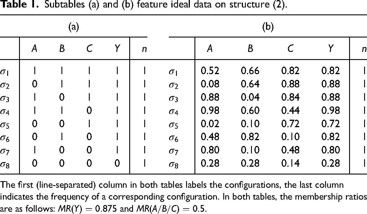
Subtables (a) and (b) feature ideal data on structure (2).

(a)						(b)
	$A$	$B$	$C$	$Y$	$n$		$A$	$B$	$C$	$Y$	$n$
${\sigma }_1$	1	1	1	1	$1$	${\sigma }_1$	0.52	0.66	0.82	0.82	$1$
${\sigma }_2$	0	1	1	1	$1$	${\sigma }_2$	0.08	0.64	0.88	0.88	$1$
${\sigma }_3$	1	0	1	1	$1$	${\sigma }_3$	0.88	0.04	0.84	0.88	$1$
${\sigma }_4$	1	1	0	1	$1$	${\sigma }_4$	0.98	0.60	0.44	0.98	$1$
${\sigma }_5$	0	0	1	1	$1$	${\sigma }_5$	0.02	0.10	0.72	0.72	$1$
${\sigma }_6$	0	1	0	1	$1$	${\sigma }_6$	0.48	0.82	0.10	0.82	$1$
${\sigma }_7$	1	0	0	1	$1$	${\sigma }_7$	0.80	0.10	0.48	0.80	$1$
${\sigma }_8$	0	0	0	0	$1$	${\sigma }_8$	0.28	0.28	0.14	0.28	$1$

The first (line-separated) column in both tables labels the configurations, the last column indicates the frequency of a corresponding configuration. In both tables, the membership ratios are as follows: $MR(Y)=0.875$ and $MR(A/B/C)=0.5$ .

The Problem of Imbalanced Data

As difference-making pairs are the main drivers of CNA’s inference to causation, the value distributions of factors above and below the 0.5-anchor may affect CNA’s performance. Notably in extreme scenarios, where all values of $\mathrm{X}$ or $\mathrm{Y}$ are above or below the 0.5-anchor, the data do not contain any difference-making pairs whatsoever, for the simple reason that all cases are uniformly in or out of $X$ and $Y$ . Without differences in set memberships, no difference-making pairs and, thus, no difference-making evidence. In order for data to contain reliably exploitable difference-making evidence, the value distributions of analyzed factors must be balanced so that an appropriate number of cases fall above and below the 0.5-anchor. Of course, the exact meaning of “appropriate” requires specification—which is the very topic of this paper.

Based on Oana et al. (2021), we define the membership ratio ( $MR$ ) in a crisp or fuzzy set $X$ to be the ratio of cases in data $\delta$ with X $>0.5$ to all cases in $\delta$ . ⁴ For example, $MR(X)=0.8$ means that $\mathrm{X}$ takes a value $>0.5$ in 80% of the cases in $\delta$ and a value $\le 0.5$ in 20% of the cases. Whenever the value distributions of a factor do not partition the cases in the data into sets of roughly equal size, we speak of an imbalanced (or skewed) factor distribution. Imbalanced distributions come in degrees and are the higher the farther away membership ratios are from $0.5$ . However, data imbalances are the norm in applied research and most of them are unproblematic because they do not impair CNA’s performance. For $\delta$ to contain an appropriate amount of difference-making evidence, it suffices that membership ratios lie in some interval centered around 0.5. A factor $\mathrm{X}$ only counts as problematically imbalanced if the membership ratio in $X$ is outside of this moderate interval. Problematic imbalances are those imbalances that our subsequent investigation shows to significantly weaken CNA’s performance, on average.

For QCA, Oana et al. (2021) propose that “as a rule of thumb” (p. 48) ratios outside of the interval $[0.8,0.2]$ are problematic. But they do not provide an argument for why this, rather than, say, $[0.9,0.1]$ is the relevant interval and they stress themselves that these are not fixed thresholds. Moreover, as there are many algorithmic differences between CNA and QCA (Swiatczak, 2022), the question as to the interval outside of which membership ratios should be considered problematic is entirely open for CNA at this point. Note that the CCM literature typically discusses data imbalances under the label of skewness (e.g., Schneider and Wagemann, 2012; Oana et al., 2021; Thomann and Maggetti, 2020), which must not be confused with skewness in statistics, where it is a measure for the asymmetry of the distribution of a variable around its mean (e.g., Tabachnick and Fidell, 2019). What matters for difference-making evidence in CCMs, however, are neither distributional symmetries nor mean factor values, but only the ratios of cases above and below the 0.5-anchor. ⁵ For that reason, we prefer to speak of data imbalances or imbalanced distributions. Even so, we acknowledge that the term skewness has an established usage in CCMs and, occasionally, also speak of skewness or skewed distributions. ⁶

The Case of Ideal Data

Before turning to the problem of demarcating the interval of problematic membership ratios, the special case of ideal data requires separate treatment. The reason is that, in ideal data, membership ratios can be extreme without any negative consequences for the performance of CNA. To see this, we first have to specify when data are ideal in configurational causal modeling. This is best accomplished by example. Thus, assume that the behavior of the factors in the set ${\mathbf{F}}_1=\{\text{A},\text{B},\text{C},\text{Y}\}$ is regulated by the causal structure corresponding to this simple MINUS-formula, which we will refer to as the ground truth:

$$A+B+C\leftrightarrow Y$$

(2)(2) entails that $A$ , $B$ , and $C$ are three alternative causes of $Y$ . If we take the factors in ${\mathbf{F}}_1$ to be crisp-set and hold additional causes of $Y$ not contained in ${\mathbf{F}}_1$ constant, it follows that the factors in ${\mathbf{F}}_1$ can be combined in exactly the eight configurations listed in Table 1a. To generalize for the fuzzy-set case, Table 1b contains fuzzy-set data corresponding to the crisp-set configurations in Table 1a. As the factors in ${\mathbf{F}}_1$ take a value above the 0.5-anchor in one of these tables exactly if they take such a value in the other one, both tables feature the same configurations.

There are $2^3=8$ logically possible ways of combining values above and below the 0.5-anchor of the 3 exogenous factors in (2), all of which are contained in Tables 1a and 1b. Moreover, these tables do not contain any configurations incompatible with (2), that is, (2) is true in all configurations of both tables. ⁷ It follows that Tables 1a and 1b feature neither fragmentation nor noise. ⁸ Fragmentation of a data set $\delta$ generated by a ground truth $\mathrm{\Delta }$ over a factor set ${\mathbf{F}}_i$ is defined as the ratio of configurations of the factors in ${\mathbf{F}}_i$ compatible with $\mathrm{\Delta }$ that are missing from $\delta$ . By contrast, data $\delta$ feature noise when some configurations in $\delta$ are incompatible with $\mathrm{\Delta }$ , which obtains if the left-hand and right-hand sides of the ’ $\leftrightarrow$ ’ in the MINUS-formula corresponding to $\mathrm{\Delta }$ , $lhs(\mathrm{\Delta })$ and $rhs(\mathrm{\Delta })$ , are non-identical (e.g., due to measurement error or confounding). The higher the mean differences between $lhs(\mathrm{\Delta })$ and $rhs(\mathrm{\Delta })$ in $\delta$ , the higher $\delta$ ’s noise level. Accordingly, noise can be measured in terms of the mean absolute difference between $lhs(\mathrm{\Delta })$ and $rhs(\mathrm{\Delta })$ in the $n$ cases of $\delta$ :

$$\frac{{\sum }_{i=1}^n|lhs(\mathrm{\Delta }{)}_i-rhs(\mathrm{\Delta }{)}_i|}{n}$$

(3)Data with zero fragmentation and zero noise are ideal data. Thus, Tables 1a and 1b contain ideal data on ground truth (2) with each configuration realized by exactly one case. While the distributions of the exogenous factors are balanced in both tables, Y takes a value above $0.5$ in 7 of 8 cases, yielding $MR(Y)=0.875$ . That is, even though Tables 1a and 1b contain ideal data, they feature an endogenous factor that is imbalanced to a degree that counts as problematic for QCA subject to Oana et al.’s (2021) rule of thumb. Clearly though, this extreme imbalance is all but problematic. Rather, it is induced by the form of the ground truth (2) itself. If case frequencies are kept constant, that is, if we ensure that all configurations are realized by an equal amount of cases, ideal data on structure (2) will always have very high membership ratios in Y. Despite the extreme imbalance of Y, CNA easily infers the MINUS-formula (2) from Tables 1a and 1b. Factor Y is imbalanced because, subject to the ground truth (2), there are three independent paths to produce $Y$ , each of which is activated by simply instantiating one cause. That means the overwhelming majority of all logically possible configurations of the exogenous factors produce $Y$ , which, correspondingly, occurs frequently in ideal data with constant case frequencies.

Plainly, not only high but also low membership ratios can be induced by the structure of the ground truth. Assume that, instead of (2), the following is the ground truth:

$$A*B*C\leftrightarrow Y$$

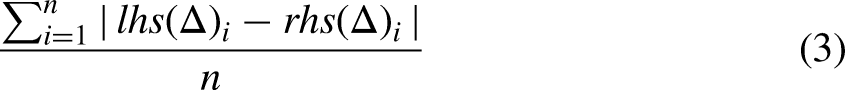
(4)If the three causes of $Y$ are not disjunctively concatenated as in (2) but conjunctively as in (4), three factors must jointly take values above 0.5 for $Y$ to occur, which only happens in one of eight configurations in the ideal data on (4) in Tables 2a and 2b, where the membership ratio in $Y$ is $MR(Y)=0.125$ , while $MR(A)$ , $MR(B)$ , and $MR(C)$ are again perfectly balanced at $0.5$ . Just as in case of Table 1, CNA straightforwardly infers (4) from Tables 2a and 2b.

Table 2.

Subtable (a) features ideal crisp-set data on structure (4), subtable (b) ideal fuzzy-set data on structure (4), and subtable (c) comprises ideal crisp-set data, with unequal case frequencies, on structure (4).

(a)						(b)						(c)
	$A$	$B$	$C$	$Y$	$n$		$A$	$B$	$C$	$Y$	$n$		$A$	$B$	$C$	$Y$	$n$
${\sigma }_1$	1	1	1	1	$1$	${\sigma }_1$	0.60	0.84	0.64	0.60	$1$	${\sigma }_1$	1	1	1	1	$33$
${\sigma }_2$	0	1	1	0	$1$	${\sigma }_2$	0.20	0.66	0.56	0.20	$1$	${\sigma }_2$	0	1	1	0	$1$
${\sigma }_3$	1	0	1	0	$1$	${\sigma }_3$	0.90	0.10	0.86	0.10	$1$	${\sigma }_3$	1	0	1	0	$1$
${\sigma }_4$	1	1	0	0	$1$	${\sigma }_4$	0.86	0.96	0.04	0.04	$1$	${\sigma }_4$	1	1	0	0	$1$
${\sigma }_5$	0	0	1	0	$1$	${\sigma }_5$	0.16	0.36	0.88	0.16	$1$	${\sigma }_5$	0	0	1	0	$1$
${\sigma }_6$	0	1	0	0	$1$	${\sigma }_6$	0.14	0.58	0.38	0.14	$1$	${\sigma }_6$	0	1	0	0	$1$
${\sigma }_7$	1	0	0	0	$1$	${\sigma }_7$	0.68	0.14	0.04	0.04	$1$	${\sigma }_7$	1	0	0	0	$1$
${\sigma }_8$	0	0	0	0	$1$	${\sigma }_8$	0.24	0.24	0.00	0.00	$1$	${\sigma }_8$	0	0	0	0	$1$

The first (line-separated) column in all subtables labels the configurations, the last column indicates the frequency of a corresponding configuration. The data in (a)-(b) have membership ratios of $MR(Y)=0.125$ and $MR(A/B/C)=0.5$ , the data in (c) have $MR(Y)=0.825$ and $MR(A/B/C)=0.9$ .

In general, membership ratios in outcomes in ideal data ${\delta }^{id}$ with constant case frequencies depend on the structural properties of the ground truth $\mathrm{\Delta }$ in the following manner: Given a fixed number of conjuncts in $\mathrm{\Delta }$ , the more disjuncts $\mathrm{\Delta }$ has, the higher the membership ratio in the outcome in ${\delta }^{id}$ , as the outcome can be produced more easily (via more paths), that is, more frequently. Conversely, given a fixed number of disjuncts in $\mathrm{\Delta }$ , the more conjuncts $\mathrm{\Delta }$ has, the lower the membership ratio in the outcome in ${\delta }^{id}$ , as more conditions must be satisfied to produce the outcome, which is more difficult to accomplish and, correspondingly, occurs less frequently. We refer to imbalances that are induced by the properties of the ground truth as structure-induced. Note that, in ideal data with constant case frequencies, exogenous factors are always perfectly balanced, even when endogenous factors are affected by structure-induced imbalances.

However, ideal data are not required to have constant case frequencies. Some configurations may be realized by more cases than others in ideal data. To illustrate, consider Table 2c, which, like Table 2a, contains ideal crisp-set data on structure (4). But while all configurations in Tables 2a and 2b are realized by exactly one case, in Table 2c, configuration ${\sigma }_1$ is realized much more frequently than all others (i.e., by 33 cases). This mismatch in case frequencies is not due to structural properties of (4), rather, cases realizing configuration ${\sigma }_1$ just happen to be more frequent than cases realizing the other configurations. The frequency mismatch in Table 2c yields that all membership ratios are high: $MR(Y)=0.825$ and $MR(A/B/C)=0.9$ . Plainly, if configuration ${\sigma }_8$ instead of ${\sigma }_1$ was realized more frequently, the result would not be high but low membership ratios. We refer to imbalances that are not induced by the properties of the ground truth as frequency-induced. As the example in Table 2c demonstrates, both exogenous and endogenous factors can be affected by frequency-induced imbalances in ideal data. But importantly, what we showed for CNA’s analysis of Tables 1a, 1b, 2a, and 2b also holds for Table 2c: The MINUS-formula inferred by CNA corresponds to the ground truth.

Overall, extreme imbalances, whether structure- or frequency-induced, do not impair CNA’s performance provided that the data are free of fragmentation and noise, that is, ideal. As indicated in the last section, difference-making pairs of configurations constitute the main inferential lever of CNA. Ideal data contain exactly those difference-making pairs that are characteristic for the underlying ground truth. How often factors take values above the 0.5-anchor or how frequently configurations are realized by cases is irrelevant for the difference-making evidence contained in ideal data and, correspondingly, for CNA’s analysis of such data. If the data contain all and only the difference-making pairs compatible with a ground truth, the latter will always be recovered by CNA. A demonstration of this is provided in an R-script contained in the paper’s supplemental online materials.

The same cannot be expected for fragmented or noisy data. CNA has to fit its models to non-ideal data by lowering the thresholds on its fit measures of consistency and coverage (Baumgartner and Ambühl, 2020), and these measures are sensitive to distributional imbalances generated by case frequencies. Frequency-induced imbalances may push consistency and coverage scores up or down in non-ideal data, thereby distort the signal in the data, and make it difficult to distinguish signal from noise. In the following simulation experiments we determine how data imbalances affect CNA’s performance when analyzing non-ideal data.

Simulation Experiments

We run a series of simulation experiments benchmarking the performance of CNA with noisy or fragmented data featuring varying degrees of distributional imbalances. The experiments are designed as inverse search trials. That is, we first randomly draw ground truths, second, simulate data from these ground truths featuring systematically varied membership ratios in all possible combinations with noise or fragmentation—which we hold constant in most of the trials—, third, analyze the data with CNA, and fourth, measure how frequently the ground truths (or proper parts thereof) are contained in CNA’s output. We use the implementation of CNA in the R-libraries cna and frscore (Ambühl and Baumgartner, 2023; Parkkinen, Baumgartner, and Ambühl, 2021). The code of the test series is available in the paper’s supplemental online materials.

Test Setup and Data Simulation

The series consists of four experiments, which differ in the investigated data characteristics. The data analyzed in all experiments are simulated from a stock of 1,000 ground truths ${\mathrm{\Delta }}_1$ to ${\mathrm{\Delta }}_{1000}$ , randomly drawn from the factor set ${\mathbf{F}}_2=\{\text{A, B, C, D, E, F}\}$ . As the execution time of the CNA algorithm increases, on average, with the complexity of the models to be built and as we process a total of over 100,000 data sets in the whole series, we have to restrict the maximal complexity of the ground truths ${\mathrm{\Delta }}_i$ . Hence, our ${\mathrm{\Delta }}_i$ have one outcome only and a maximum of three alternative paths (i.e., disjuncts), with a maximum of three causes on each path (i.e., conjuncts), producing the outcome. While many real-life CNA applications actually target causal structures within that complexity range, it must also be emphasized that this restriction has consequences for our experiments. Ground truths drawn within that complexity range tend to have endogenous factors with slightly structure-induced imbalances. More precisely, the average membership ratio in the outcome in ground truths satisfying our complexity restriction is about 0.4. How this affects our findings will be discussed in the results section. Finally, to test how frequently data imbalances induce CNA to erroneously include causally irrelevant factor values (i.e., non-causes) in its models, we ensure that, in all ${\mathrm{\Delta }}_i$ , there is at least one element of ${\mathbf{F}}_2$ missing, values of which, thus, are causally irrelevant.

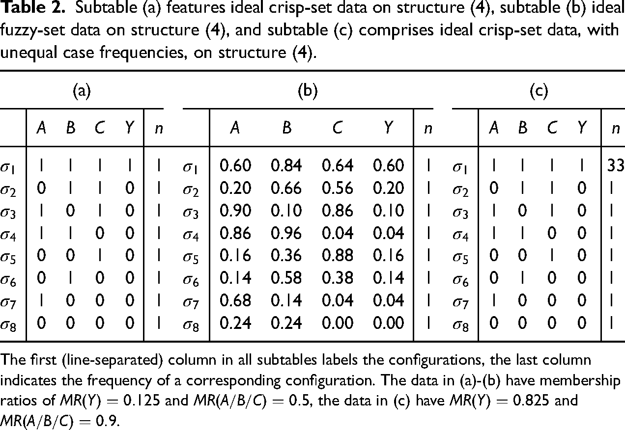
The first step of the data simulation process then is the same in all four experiments: For every ${\mathrm{\Delta }}_i$ , we generate ideal fuzzy-set data on the factors in ${\mathbf{F}}_2$ , with a sample size of 50 cases each, yielding 1,000 ideal data sets ${\delta }_1^{id}$ to ${\delta }_{1000}^{id}$ . For every ${\delta }_i^{id}$ it holds that the left- and right-hand sides of the MINUS-formula corresponding to ${\mathrm{\Delta }}_i$ have identical membership scores in each row of ${\delta }_i^{id}$ and that all configurations compatible with ${\mathrm{\Delta }}_i$ are represented by at least one case in ${\delta }_i^{id}$ . In the second and third step, we add noise or fragmentation to ${\delta }_i^{id}$ (see Table 3). In experiment 1, we add fragmentation but no noise, in experiment 2, we add noise but no fragmentation, and in experiments 3 and 4 we add both fragmentation and noise. Contrary to experiments 1, 2, and 3, where fragmentation is kept constant at the expense of varying sample sizes, we keep sample sizes constant in experiment 4 and allow fragmentation to vary.

Table 3.

Overview of investigated data characteristics in experiments 1-4.

	Experiment 1	Experiment 2	Experiment 3	Experiment 4
Resulting mean noise ratio randomly introduced from $[0,0.3]$ 9	0	$0.15$	$0.15$	$0.15$
Resulting mean fragmentation ratio randomly introduced from $[0.2,0.5]$	$0.35$	0	$0.35$	$0.21-0.41$
Resulting mean sample size	$23-123$	$53-282$	$36-182$	57
Manipulated membership ratios (MR)	$MR(OUT)$ , $MR(CAU)$ , $MR(nonCAU)$ varied to each value in $⟨0.1,0.2,0.3,0.4,0.5,0.6,0.7,0.8,0.9⟩$

The first two rows indicate if noise or fragmentation was added. In experiments 1-3, fragmentation is kept constant at the expense of varying sample sizes. In experiment 4, sample size is kept constant at the expense of varying fragmentation ratios.

Whenever noise or fragmentation are introduced, this is done at random. To randomly introduce noise into ${\delta }_i^{id}$ , we first draw a number $\gamma$ from the interval $[0,0.3]$ . Second, we draw a sequence $ϵ$ of normally distributed random errors from the interval $[-1,1]$ with a length equal to the number of rows of ${\delta }_i^{id}$ such that, over all rows of ${\delta }_i^{id}$ , the mean absolute difference between the scores of $lhs({\mathrm{\Delta }}_i)$ and $lhs({\mathrm{\Delta }}_i)+ϵ$ is equal to $\gamma$ . Third, we replace the outcome value in every row $j$ of ${\delta }_i^{id}$ by the sum of that outcome value and the $j^{th}$ element of $ϵ$ . The resulting data have a noise ratio equal to $\gamma$ , meaning anywhere between $0$ and $0.3$ . To randomly fragment a data set ${\delta }_i^{id}$ , we draw a ratio from the interval $[0.5,0.8]$ and sample that ratio of configurations from ${\delta }_i^{id}$ (without replacement). The resulting data have a fragmentation ratio anywhere between $0.2$ and $0.5$ . The upshot of introducing noise or fragmentation into each ${\delta }_i^{id}$ in accordance with the requirements of the different experiments are $4\times 1,000$ non-ideal base data sets of type ${\delta }_i^k$ , where $k$ refers to the experiment and $i$ numbers the data set. For example, ${\delta }_{543}^2$ designates the ${543}^{rd}$ base data for experiment 2.

In these base data sets, we then, in the fourth step, systematically manipulate case frequencies in order to modify selected membership ratios such that these ratios are transformed to each value in the following variation sequence:

$$⟨0.1,0.2,0.3,0.4,0.5,0.6,0.7,0.8,0.9⟩.{}^1{}^0$$

This is done in three different legs of each experiment. In the first leg, case frequencies in ${\delta }_i^k$ are manipulated such that the membership ratio in the outcome (OUT) is transformed to each value of the variation sequence. In the second leg, a cause (CAU) is randomly selected in each ${\delta }_i^k$ and frequencies in ${\delta }_i^k$ manipulated such that the membership ratio in that cause assumes all values in the variation sequence. In the third leg, a non-cause (nonCAU) is selected in each ${\delta }_i^k$ and its membership ratio correspondingly transformed. That is, in every leg of an experiment, 9 (length of the variation sequence) frequency-manipulated data sets are built from every base set ${\delta }_i^k$ . As there are three legs in each of the four experiments, we end up with $9\times 3\times 4\times 1,000=108,000$ test data sets for the whole series. We will refer to them by ${\delta }_{t/i}^{k/r}$ , where $k$ indicates the experiment, $r$ the targeted membership ratio, $t$ the leg of the experiment, and $i$ numbers the data. For example, ${\delta }_{3/34}^{2/0.4}$ designates the 34 ${}^{th}$ data set in the 3 ${}^{rd}$ leg of experiment 2, in which the membership ratio in a non-cause is transformed to $0.4$ .

As these data transformations are done by changing case frequencies in the base data, all resulting membership ratios are frequency-induced. In experiments 1–3, case frequencies are modified by suitably selecting cases from the base ${\delta }_i^k$ in such a way that the fragmentation and noise ratios of ${\delta }_i^k$ are retained (as closely as possible) in the transformed data ${\delta }_{t/i}^{k/r}$ . Depending on what the initial membership ratio is in ${\delta }_i^k$ , this selection process may cause ${\delta }_{t/i}^{k/r}$ to have a much larger sample size than ${\delta }_i^k$ . Also, the sample sizes of the test data vary greatly within each leg of an experiment. On average, test sets at the lower and upper ends of the variation sequence have much larger sample sizes than test sets targeting membership ratios around $0.5$ .

As sample sizes may influence the performance of CNA, experiment 4 varies membership ratios in such a way that, apart from noise ratios, also sample sizes are held constant across all data transformations. Selecting cases from the base set ${\delta }_i^k$ in such a way that noise and sample size stay the same can only be accomplished at the expense of varying fragmentation. That is, the test data ${\delta }_{t/i}^{k/r}$ may have much higher fragmentation than the corresponding base ${\delta }_i^k$ and fragmentation also varies within each leg of an experiment. Test sets targeting membership ratios around $0.5$ tend to have lower fragmentation than sets aiming for extreme ratios. Table 3 summarizes the settings for the four experiments.

Data Analysis and Benchmark Criteria

The 108,000 test data sets are analyzed by CNA using the robustness analysis protocol developed by Parkkinen and Baumgartner (2023). That means that each ${\delta }_{t/i}^{k/r}$ is not only analyzed at one designated tuning setting of consistency and coverage thresholds but re-analyzed at all settings in a whole sequence of consistency and coverage thresholds. For our analysis we choose the sequence $⟨0.65,0.70,0.75,\dots ,1⟩$ . All MINUS-formulas CNA recovers in that re-analysis series are collected and their robustness and overall model fit measured and scored. For every ${\delta }_{t/i}^{k/r}$ , we then return the $95$ ^th percentile of top-performing MINUS-formulas as CNA’s output set $\mathbf{S}$ for that data.

The elements of such a set, which contains between 1 and 6 models in our test series, are indistinguishable on the basis of the evidence contained in ${\delta }_{t/i}^{k/r}$ by current model selection standards used in CNA. Accordingly, if $\mathbf{S}$ comprises more than one MINUS-formula, CNA cannot determine which of those formulas truthfully represents the ground truth ${\mathrm{\Delta }}_i$ ; all that can be said is that at least one of them is true of ${\mathrm{\Delta }}_i$ . It follows that a set $\mathbf{S}$ featuring, say, three MINUS-formulas ${\mathbf{m}}_1$ , ${\mathbf{m}}_2$ , and ${\mathbf{m}}_3$ is to be causally interpreted disjunctively: ${\mathbf{m}}_1$ OR ${\mathbf{m}}_2$ OR ${\mathbf{m}}_3$ is true of ${\mathrm{\Delta }}_i$ . ¹¹ If CNA returns multiple models in a real-life discovery context, an analyst has to rely on data-external sources of information as theoretical background knowledge to select among the candidates. ¹² As such a data-external background is not available for simulated data, we take the set $\mathbf{S}$ inferred from ${\delta }_{t/i}^{k/r}$ to be CNA’s final output for these data. All in all, analyzing the data of our entire test series yields 108,000 output sets ${\mathbf{S}}_i$ .

We assess the quality of all those output sets based on three complimentary benchmark criteria, which Table 4 summarizes. The first is a qualitative correctness criterion, which has been repeatedly used in CCM benchmarking before (e.g., Baumgartner and Ambühl, 2020; Baumgartner and Thiem, 2020; Baumgartner and Falk, 2023).

Table 4.

Overview of used benchmark criteria with example formulas that (do not) pass respective criteria assuming that (1), i.e. $A*b+c*D\leftrightarrow E$ , is the ground truth.

Criterion	Substance	Output	Examples based on (1)
Correctness	non-empty output without false positives	(not) passed	passed: $A*b\leftrightarrow E$ ; $A+D\leftrightarrow E$ not passed: $A*B\leftrightarrow E$ ; $A+b\leftrightarrow E$
Completness	degree of ground truth captured	passed to degree	$A*b\leftrightarrow E$ ; $A+D\leftrightarrow E$ both score $2/4=0.5$
Error-freeness	no false positives or empty output	(not) passed	passed: $A*b\leftrightarrow E$ ; $\mathrm{\varnothing }$ not passed: $A*B\leftrightarrow E$

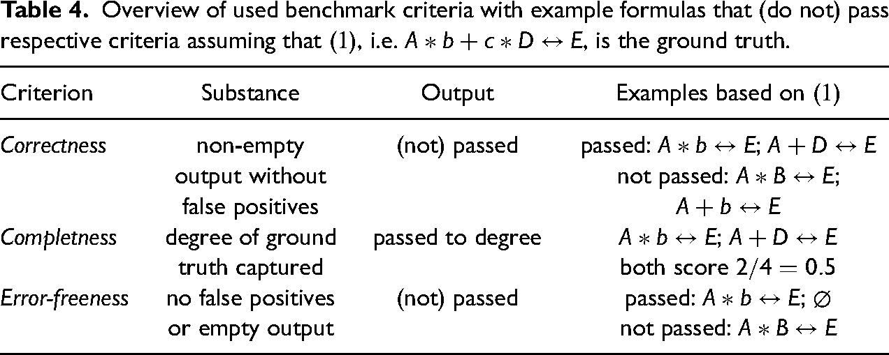
According to that criterion, what CNA infers from ${\delta }_{t/i}^{k/r}$ counts as correct if, and only if, that inference is true of the underlying ground truth ${\mathrm{\Delta }}_i$ . As we have seen above, that is the case if, and only if, at least one MINUS-formula ${\mathbf{m}}_j$ in ${\mathbf{S}}_i$ is true of ${\mathrm{\Delta }}_i$ , which, in turn, holds if, and only if, all factor values contained in ${\mathbf{m}}_j$ are in fact causes of the outcome of ${\mathrm{\Delta }}_i$ and all conjunctive and disjunctive groupings in ${\mathbf{m}}_j$ are in agreement with ${\mathrm{\Delta }}_i$ . In other words, ${\mathbf{m}}_j$ is correct if, and only if, it entails no false positives. ¹³ For example, if formula (1) from our previous example, i.e. $A*b+c*D\leftrightarrow E$ , is the ground truth, models as $A*b\leftrightarrow E$ or $A+D\leftrightarrow E$ are correct because all factor values contained in these models are in fact causes of $E$ and all conjunctive and disjunctive groupings are true of (1). By contrast, a model as $A*B\leftrightarrow E$ is incorrect because $B$ is not in fact a cause of $E$ , or $A+b\leftrightarrow E$ is incorrect because $A$ and $b$ are conjunctively and not disjunctively grouped in (1). If CNA does not infer anything from ${\delta }_{t/i}^{k/r}$ and, thus, ${\mathbf{S}}_i$ is empty—say, because consistency or coverage thresholds cannot be met— ${\mathbf{S}}_i$ does not pass the correctness benchmark.

The second benchmark is a completeness criterion that quantifies the informativeness of correct MINUS-formulas. Making only true claims about ${\mathrm{\Delta }}_i$ , as is required to pass the correctness benchmark, can be easily accomplished by models that make only very few causal claims. Also, of two correct MINUS-formulas one can be more complex than the other and, hence, reveal ${\mathrm{\Delta }}_i$ more completely. As more informative models are preferable, the completeness benchmark measures the degree to which the correct MINUS-formulas in ${\mathbf{S}}_i$ exhaustively reveal ${\mathrm{\Delta }}_i$ . More specifically, completeness amounts to the ratio of the complexity of the most complex correct MINUS-formula in ${\mathbf{S}}_i$ to the complexity of ${\mathrm{\Delta }}_i$ , where complexity of a MINUS-formula ${\mathbf{m}}_i$ is understood as the number of factor values in ${\mathbf{m}}_i$ . That is, contrary to correctness, which can only be either satisfied or not, the second benchmark can be passed by degree. For example, if (1) is the ground truth, models as $A*b\leftrightarrow E$ or $A+D\leftrightarrow E$ score $2/4=0.5$ on completeness, as they recover two of the four factor values contained in the ground truth. When ${\mathbf{S}}_i$ is either empty or does not contain a correct MINUS-formula, completeness is 0 by default.

As a supplement, we measure a third auxiliary criterion, error-freeness, that is also qualitative and counts as passed if, and only if, ${\mathbf{S}}_i$ as a whole is not false. Contrary to correctness and completeness, error-freeness is non-zero both if ${\mathbf{S}}_i$ contains a MINUS-formula ${\mathbf{m}}_i$ that does not entail a false positive and if ${\mathbf{S}}_i$ is empty. As an empty output set is uninformative and thus suboptimal, error-freeness is not a benchmark on a par with correctness and completeness, and our subsequent discussion will mainly focus on the latter two benchmarks. Nonetheless, error-freeness deserves some attention because an empty output is still preferable over a false one.

Results

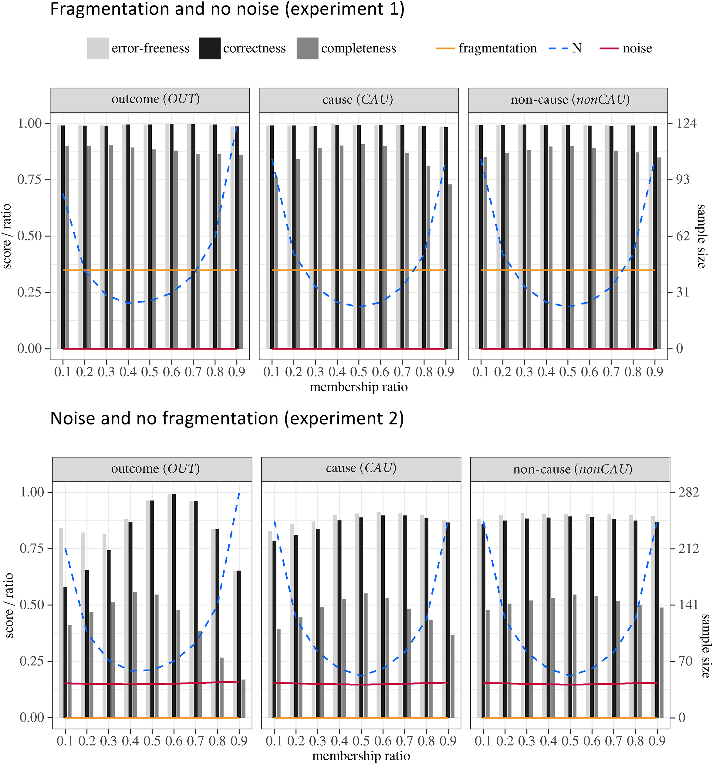
The results of experiments 1 and 2 are plotted in the bar-charts in Figure 1, Figure 2 shows the results of experiments 3 and 4. Black bars represent correctness scores, dark gray bars completeness scores, and light gray bars depict error-freeness scores. The effects of varying membership ratios in an outcome, a cause, and a non-cause are presented in separate panels. The exact values of all scores can be found in the score tables in the paper’s supplemental online materials. Apart from the benchmark scores, the plots also display fragmentation and noise ratios as well as sample sizes. All values are means over 1,000 CNA analyses of 1,000 test data ${\delta }_{t/i}^{k/r}$ . For example, the correctness score of 0.99 depicted by the first (black) bar in the leftmost panel in the plot of experiment 1 in Figure 1 means that CNA found a correct MINUS-formula for 99% of the 1,000 test data of type ${\delta }_{1/i}^{1/0.1}$ . The fragmentation score of 0.35 superimposed over that bar means that, on average, 35% of rows compatible with the corresponding ground truths are missing from the 1,000 ${\delta }_{1/i}^{1/0.1}$ . ¹⁴

Figure 1.

Results of experiments 1 and 2, subdivided by their three legs. Membership ratios are plotted on the $x$ -axis, benchmark scores (black and shades of gray), noise (red), and fragmentation ratios (orange) are on the left $y$ -axis, sample sizes (blue) on the right $y$ -axis. All values are means over 1,000 CNA runs.

Figure 2.

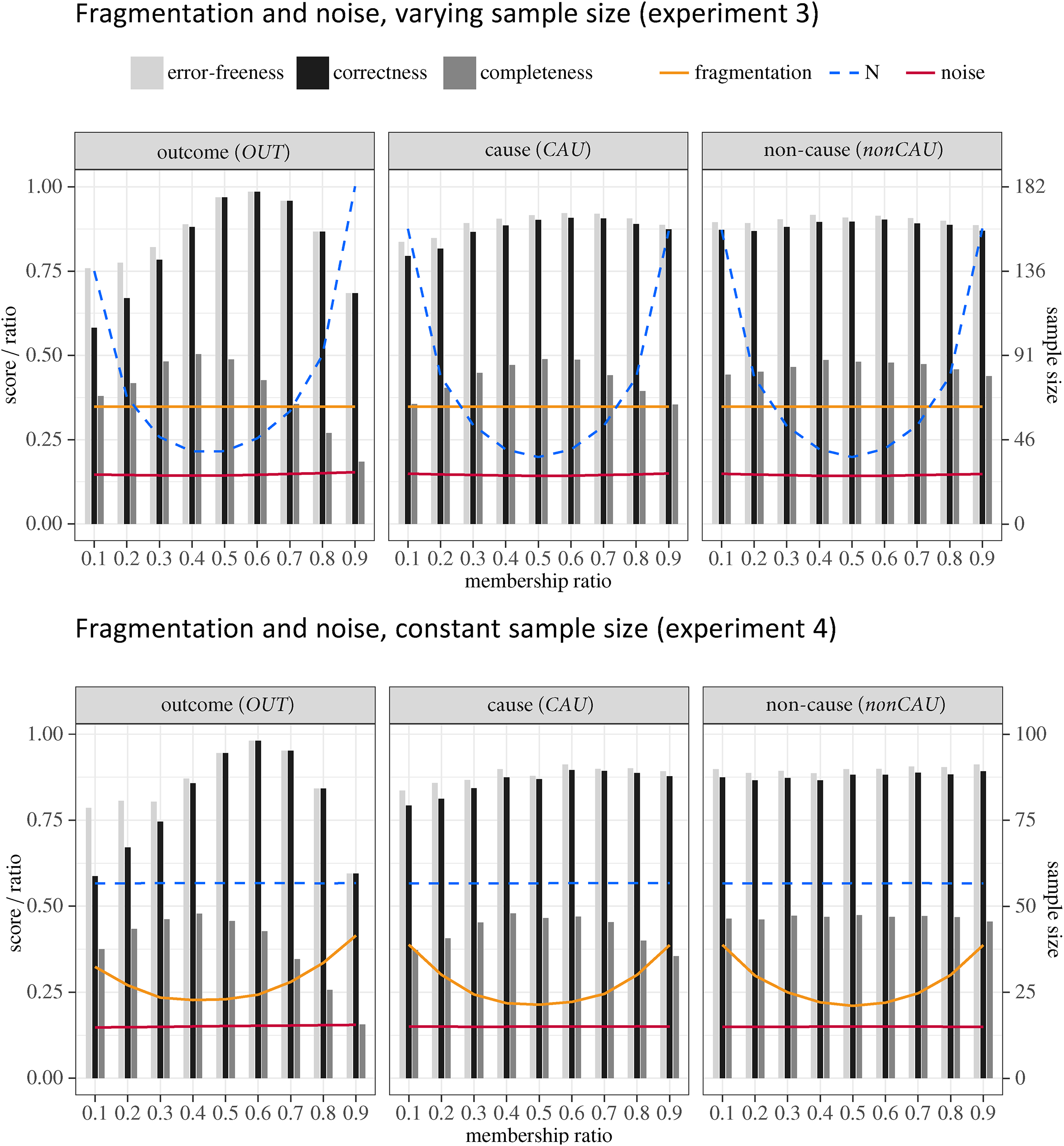
Results of experiments 3 and 4, subdivided by their three legs. Membership ratios are plotted on the $x$ -axis, benchmark scores (black and shades of gray), noise (red), and fragmentation ratios (orange) are on the left $y$ -axis, sample sizes (blue) on the right $y$ -axis. All values are means over 1,000 CNA runs.

First and foremost, our results demonstrate, that increasing distributional imbalances may be associated with decreasing performance even when fragmentation, noise, or sample size are kept constant. This, in turn, shows that data imbalances do not only exacerbate the negative effects of other data deficiencies but also have an independent negative effect. In what follows, we break this main finding down in more detail.

Fragmentation vs. Noise

Data imbalances have weaker effects when paired only with fragmentation than when paired with noise. In all three legs of experiment 1, where fragmented but noise-free data are processed, correctness scores remain almost maximal (between 0.98 and 1). Maximal completeness, however, cannot be achieved because of the fragmentation, which amounts to missing empirical information about ground truths ${\mathrm{\Delta }}_i$ . In legs 1 and 3, varying membership ratios only barely affect completeness scores (which remain between 0.85 and 0.90) beyond the impact of fragmentation. In leg 2, distributional imbalances drag completeness down noticeably. If $MR(CAU)$ is set to $0.1$ or $0.2$ , the cause is so rare that it is no longer needed to cover the outcome and thus is not built into the models. By contrast, in the trials with $MR(CAU)=0.8/0.9$ , the cause is so frequent that it covers the outcome even without other causes, which therefore become redundant and are not built into the models. In both scenarios, some causes are missing from CNA’s models in addition to those that are missing due to fragmentation alone.

In experiments 2–4, where data feature noise, both correctness and completeness scores drop significantly compared to experiment 1 because CNA cannot persistently avoid false positives in the presence of noise, which, after all, amounts to incorrect information about ${\mathrm{\Delta }}_i$ . Moreover, in trials when all models in ${\mathbf{S}}_i$ make false claims about ${\mathrm{\Delta }}_i$ , both correctness and completeness are 0. Completeness drops more than correctness because CNA is designed to keep false positives to a minimum, meaning that the method abstains from including a factor value in a model, if its causal relevance is not sufficiently corroborated by the data. The more cautiously a method operates, the less causal inferences it draws, the lower the chances that false positives are committed, yet the less completely ${\mathrm{\Delta }}_i$ is recovered.

Owing to its cautiousness, CNA frequently abstains from drawing any inferences when the outcome is very rare in experiments 2–4. The result are empty output sets ${\mathbf{S}}_i$ in up to 25% of the trials, which can be read off the large difference in correctness and error-freeness scores at the lower end of the variation sequence. Error-free trials that do not pass correctness are trials with empty outputs. In consequence, error-freeness scores remain above 0.75 in all experiments even when the outcome is very rare. By contrast, when $MR(OUT)=0.9$ , there are no longer any empty outputs, to the effect that error-freeness and correctness coincide and drop well below 0.75. The reason is overfitting. Due to the noise, conjunctions of only one or two factor values are not consistently sufficient for the outcome, such that CNA builds rather complex minimally sufficient conditions, on average. And in order to cover a very frequent outcome with complex conditions, large disjunctions of many of these conditions are needed. In 35%–40% of the trials on noisy data at $MR(OUT)=0.9$ , CNA’s output sets contain only overfitted models.

Performance Peaks

Another feature of the results obtained in the first leg of experiments 2–4 is that, across all variations of $MR(OUT)$ , CNA scores highest on completeness at $MR(OUT)=0.4$ and highest on correctness at $MR(OUT)=0.6$ . Why are these performance peaks off-centered? To answer this question recall from the test setup that outcomes have an average structure-induced membership ratio of roughly $0.4$ in the ground truths ${\mathrm{\Delta }}_1$ to ${\mathrm{\Delta }}_{1000}$ , which, in turn, stems from the complexity restriction imposed on them. Deviations from structure-induced membership ratios in our experiments are due to biased case frequencies and hence tend not to be faithful to the structural properties of ${\mathrm{\Delta }}_i$ . The more we increase that frequency bias as we move through the variation sequence, the higher the chances that CNA builds elements into its models that fail to have counterparts in ${\mathrm{\Delta }}_i$ . The complex models contained in output sets ${\mathbf{S}}_i$ have the highest chances of being true of ${\mathrm{\Delta }}_i$ in trials at $MR(OUT)=0.4$ because, in these trials, case frequencies are manipulated the least, on average, meaning that membership ratios are most faithful to the structural properties of ${\mathrm{\Delta }}_i$ . The higher the chances that complex CNA models in ${\mathbf{S}}_i$ are true, the higher CNA’s completeness scores.

But then, why are the correctness scores, even though they are good at $MR(OUT)=0.4$ (i.e., between 0.85 and 0.88), not the highest in those trials as well? To understand that, recall that we analyze each data set at a whole range of threshold combinations, going down to consistency and coverage set to $0.65$ . The lower these thresholds, the less accurately models are required to account for the outcome, the higher the chances that very sparse models pass the thresholds. And the sparser a MINUS-formula ${\mathbf{m}}_i$ , the less causal claims it makes, which, in return, increases the probability that ${\mathbf{m}}_i$ does not make any false claims and, thus, is true of ${\mathrm{\Delta }}_i$ . The sparsest possible MINUS-formulas are one-cause formulas of type $B\leftrightarrow A$ . In our test series, CNA’s output sets contain the most one-cause formulas at $MR(OUT)=0.6$ . The fact that the MINUS-formulas with the highest a priori probability of being true are the most frequent in the trials at $MR(OUT)=0.6$ pushes CNA’s correctness score even higher than it is at $MR(OUT)=0.4$ (i.e., to scores between 0.98 and 0.99).

Outcome vs. Causes vs. Non-Causes

Finally, our results show that extreme membership ratios have varying performance impacts depending on whether they affect the outcome, a cause, or a non-cause. In all experiments, extreme membership ratios in non-causes have no significant effect on performance beyond fragmentation and noise. That means they do not induce CNA to erroneously include non-causes in models more frequently than they are included because of other data deficiencies. In contrast, extreme membership ratios in causes have sizeable effects on completeness scores in all experiments. The same mechanism as in experiment 1 accounts for this finding in all other experiments. That is, rare causes are often not included in models and frequent causes tend to render other causes redundant, which then are not included. In addition, extreme membership ratios in causes, when combined with noise (i.e., in experiments 2–4), induce a noticeable drop in correctness. Still, correctness scores do not fall below 0.79 and correctness drops are counterbalanced by error-freeness scores well above 0.8, meaning that CNA repeatedly issues no models at all.

In general, when data feature noise (i.e., in experiments 2–4) the performance impact is much higher if the endogenous factors are imbalanced than if exogenous factors are concerned. The reason is that while every ${\mathrm{\Delta }}_i$ has only one outcome, most ${\mathrm{\Delta }}_i$ have several causes, yet only the frequency of one of these is manipulated in our experiments. Thus, whereas frequency distortion in one cause can be counterbalanced by correctly inferred causal claims on other causes, this is not possible with frequency distortion in the outcome which then tends to hinder the correct recovery of the whole ${\mathrm{\Delta }}_i$ .

Discussion

We set out to answer the question whether data imbalances have their own impact on CNA’s performance. In the case of ideal data, even extreme imbalances have no such impact. However, we have seen that in case of non-ideal data, which are common in real-life research settings, extreme membership ratios affect CNA’s performance. It remains to be determined, first, which membership ratios should count as problematic for CNA, second, what counter-measures can be taken to resolve problematic distributional imbalances, and, third, what our study’s limitations are.

Demarcating Problematic Membership Ratios

In light of our results, the answer to the first question depends on an array of conditions such as the quality of the data at hand, the type of factor(s) with extreme imbalances, whether the analysts are primarily interested in correct or complete models, and how willing they are to take a risk. Accordingly, there does not exist a general and objective demarcation between problematic and unproblematic membership ratios. In what follows, we determine whether a performance drop in a particular benchmark measure within a leg of an experiment is problematic by comparing it to the best benchmark score in that leg. In order for a drop to count as problematic we require the difference to the best performance to be higher than 20%. Readers with a different assessment of what counts as problematic have to correspondingly adjust our subsequent demarcations.

If it can be plausibly assumed that the data are collected against a homogeneous background, such that noise is negligible and the only serious data deficiency is fragmentation, distributional imbalances tend not to affect performance beyond fragmentation. The only exception, as the second leg of experiment 1 shows, is that causes with extreme membership ratios noticeably reduce the completeness of CNA’s models. At $MR(CAU)=0.5$ , CNA recovers 91% of the ground truths, on average, whereas this percentage drops to 76% at $MR(CAU)=0.1$ and to 73% at $MR(CAU)=0.9$ , which amount to performance drops of 16.5% and 19.8%, respectively. Although the latter drop borders on the problem zone identified above, the fact that the overall completeness scores remain high throughout the second leg of experiment 1 lets us confidently conclude that these completeness drops, though sizeable, are not to be considered problematic.

This changes when the data are noisy. In the second leg of experiment 2, the best completeness score is 0.55 at $MR(CAU)=0.5$ ; it drops by more than 20% at $MR(CAU)=0.1$ and $MR(CAU)⩾0.8$ , and similarly in the second legs of experiments 3 and 4. Hence, in the presence of noise, membership ratios of causes outside of the interval $[0.2,0.7]$ drag down completeness to a problematic extent. It follows that somebody with an interest in learning as much as possible about the ground truth should consider countermeasures.

The same does not hold if analysts are primarily interested in correct models, that is, in reliably finding parts of the data-generating structure. While $MR(CAU)=0.9$ has no effect on correctness at all, correctness drops from a solid score of 0.9 at $MR(CAU)=0.5/0.6$ by about 12% to 0.79 at $MR(CAU)=0.1$ when the data are noisy. But at the same time, error-freeness remains between 0.83 and 0.85, meaning that the loss in correctness is to a substantive degree due to empty outputs. That is, there is a slightly increased risk of inferring something false at $MR(CAU)=0.1$ , but that increase is not severe enough to call for countermeasures against distributional imbalances; if an error risk of 15% is considered too high, taking measures against the noise in the data would be more effective.

The most problematic impact extreme membership ratios have on the correctness of CNA’s output occurs when endogenous factors are imbalanced in noisy data. In experiments 2–4, correctness and error-freeness collapse at $MR(OUT)=0.9$ . While correctness and error-freeness are between 0.84 and 0.87 at $MR(OUT)=0.8$ in the experiments with noise, these scores drop to values between 0.6 and 0.65 at $MR(OUT)=0.9$ . Compared to the best correctness scores at $MR(OUT)=0.6$ , that is a performance drop of almost 40%, down to a level where, in 2 out of 5 CNA runs, all resulting models are fallacious. That is unquestionably an instance of a problematic distributional imbalance.

The situation is not so clear in case of low membership ratios in outcomes. At $MR(OUT)=0.1/0.2$ , CNA only recovers a true model in 58%–67% of the trials, but these low correctness scores are largely due to the fact that CNA often abstains from inferring any models at all. When conditionalized on the trials that produce non-empty outputs, correctness does not fall below 0.75 at $MR(OUT)=0.1/0.2$ in any of our experiments. If a fallacy risk of 25%—in contexts where up to 30% of the observations are distorted by noise—is acceptable to the analyst, even an extremely rare outcome hence does not call for immediate countermeasures. Instead, CNA could be run to see if an output is produced. If that is not the case, the low membership ratio in the outcome is the likely source of the problem, making it an instance of a problematic imbalance after all.

Finally, at $MR(OUT)=0.1$ the completeness of the output CNA infers from noisy data is reduced by about 25%, which is deep within the problem zone. Similarly, high outcome membership ratios are very consequential for the completeness of CNA’s output in the presence of noise. At $MR(OUT)=0.7$ completeness drops between 25% and 30% compared to the optimal membership ratio; at $MR(OUT)=0.8$ completeness is cut in half, and at $MR(OUT)=0.9$ two thirds of the information CNA recovers at the optimal membership ratio are lost, on average. Hence, if maximal informativeness is a research objective and the data cannot plausibly be assumed to be noise-free, membership ratios in the outcome outside of the interval $[0.2,0.6]$ should be considered problematic.

In sum, based on our convention that performance drops need to be larger than 20% to count as problematic, we propose the following demarcation lines for problematic data imbalances, assuming a typical real-life research with the following two characteristics: First, neither fragmentation nor noise can plausibly be excluded, and second, only outcomes and candidate causes can be distinguished, but the latter cannot be grouped into causes and non-causes. If the analyst is primarily interested in finding a correct model, only $MR(OUT)=0.9$ is problematic. Yet, if the research context requires learning as much as possible about the data-generating structure, membership ratios in outcomes outside of the interval $[0.2,0.6]$ or membership ratios in candidate causes outside of the interval $[0.2,0.7]$ are problematic.

Resolving Problematic Distributional Imbalances

When it comes to taking countermeasures, problematic distributional imbalances affecting the correctness of CNA’s output must be distinguished from problematic imbalances affecting completeness. The former type requires countermeasures before CNA is applied to the data, whereas the latter type may be addressed after initial applications of CNA are found not to deliver satisfactory results. If an outcome is imbalanced at $MR(OUT)\ge 0.9$ , CNA’s output cannot be trusted in non-ideal discovery circumstances, making it imperative to take immediate action. By contrast, if the data are imbalanced in a way that does not create problems for correctness but only for completeness, say, an outcome has a membership ratio of 0.2 or 0.1, the analyst may well run an analysis and inspect the results before any action is taken. Our simulations indicate that the likelihood of not receiving any model are high. But if a non-empty output is produced under such circumstances, it may be given consideration. In fact, we have seen that such outputs are correct in 80% of the trials. Thus, if these outputs are informative enough for the research question at hand and analysts are ready to accept a fallacy risk of 20%, they can take such outputs seriously without addressing distributional imbalances. Yet, if it turns out that CNA does not return any models or that returned models are not informative enough, resolving distributional imbalances will be a promising path forward.

There are three main approaches to resolve distributional imbalances: (1) adding or removing cases, (2) adjusting membership scores via recalibration, and (3) negating values of imbalanced factors. We take them in turn. Approach (1) consists in suitably changing the sample of cases in the data. To resolve a problematically high membership ratio in $X$ , cases can be added to the data in which the factor $\mathrm{X}$ takes values below 0.5 or cases can be removed in which $\mathrm{X}$ takes values above $0.5$ . Analogously, if $MR(X)$ is problematically low, cases with membership scores above $0.5$ can be added or cases with membership scores below $0.5$ removed. Both adding and removing cases require to reassess the case selection decisions in the study design. For instance, complementing the data in a study analyzing employees from a particular industry by cases featuring employees from another (comparable) industry shifts the study’s analytical focus to employees in the union of both industries. Or, cases can be removed from that study by shifting the level of analysis from all employees in an industry to a particular group of employees from that industry, say, employees without leadership positions. Plainly, such case selection adjustments should not only be assessed based on their capacity to resolve problematic distributional imbalances but, in the first place, they must be theoretically meaningful and in line with the research interests at hand. Avoiding problematic imbalances is only one constraint among many to be taken into account when selecting cases. Moreover, note that after cases have been added or removed in order to resolve the problematic imbalance of some factor $\mathrm{X}$ , the distributions of all factors must be reassessed, not just of $\mathrm{X}$ . The reason is that changing the data basis might resolve the distributional problem for $\mathrm{X}$ but create it for another factor.

Moreover, other constraints must be kept in mind when adding and removing cases to and from the data. First, added cases should have homogenous causal backgrounds and they should be comparable to the cases already contained in the data. For example, if a study affected by problematic imbalances is concerned with Western democracies, adding cases from the set of Asian autocracies will, in all likelihood, induce homogeneity violations and, thereby, render the resulting models uninterpretable. Second, removing cases should, if possible, not increase fragmentation, that is, it should not reduce the number of configurations instantiated in the data and thus reduce the amount of difference-making evidence. In other words, cases should primarily be removed that instantiate configurations which have various other cases instantiating them in the data.

By contrast, when membership ratios are modified by recalibration in the vein of approach (2), the imbalance of one factor $\mathrm{X}$ can be tackled without affecting the distribution of the other factors. To this end, the number of $\mathrm{X}$ ’s values above and below the 0.5-anchor is changed by moving the cross-over calibration threshold defining the 0.5-anchor. If $X$ is too frequent, that threshold is moved up such that less cases are calibrated to instantiate $X$ , whereas if $X$ is too rare, the cross-over threshold is moved down such that more cases instantiate $X$ .

Note that recalibration also requires changes to the study design, as shifting calibration thresholds changes the subject matter of the analysis; it moves the analytical interest from a problematically imbalanced factor to a different, non-problematic one. Such adjustments must, of course, also be theoretically justified and in line with the study’s research goals. To illustrate, shifting the subject matter via recalibration can be an option when the imbalanced factor represents a concept for which a bias towards higher or lower values that is not induced by the causal structure under investigation can be observed. A concept as self-perceived competence (or self-efficacy) is an example for which many studies observe a general positivity bias resulting in high membership ratios (e.g., Swiatczak, 2021; Gabriel et al., 2018; Schnell, Höge, and Pollet, 2013). If the aim of the study is not to investigate the causal structure underlying overly positive competence assessments, the bias can be counterbalanced by changing the subject matter of the analysis from, say, “competent employees” to “highly competent employees”. In addition, it is clear that such recalibrations should also follow general calibration guidelines (e.g., Oana et al., 2021). Unproblematic distributions are merely one constraint among many to be considered in the calibration process.

Finally, while it can happen that approaches (1) and (2) are inapplicable because there may not be justifiable ways of changing the data basis or the calibration thresholds, approach (3) is always applicable. It amounts to simply replacing an $X$ with a problematic membership ratio by its negation $x$ , that is, $1-X$ . To illustrate, consider a scenario where $X$ is an outcome with a membership ratio of $0.7$ and an initial CNA analysis produces a model that is not informative enough. According to our findings, $X$ ’s membership ratio counts as problematic in that scenario. If $X$ is now replaced by $x$ , the previously problematic membership ratio becomes a ratio of $MR(x)=0.3$ (i.e., $1-0.7$ ), which our results show not to count as problematic. In fact, we have found that an outcome membership ratio of $0.3$ is almost optimal for completeness maximization in the presence of fragmentation and noise.

Not only is approach (3) always applicable, it also does not require intricate considerations on changing the data basis or the calibration. On the downside, however, it is not always possible to resolve problematic imbalances by simple negation. In particular, when both $X$ and $1-X$ fall into ranges of problematic membership ratios, which, according to our findings, holds if $\mathrm{X}$ is an exogenous factor, approach (3) does not solve the problem. Also, while the adjustments of the study design induced by approaches (1) and (2) may be small, negating outcomes or causes amounts to reversing the subject matter of the study entirely. It shifts the focus from investigating the presence of factors to their absence.

Limitations

Our study’s limitations originate from design decisions we had to take when simulating data. For reasons of computational feasibility, we had to restrict the complexity of the assumed ground truths to structures with one outcome and a complexity range of one to three disjuncts, each consisting of one to three conjuncts. Ground truths were randomly drawn from that complexity range to the effect that resulting ground truth complexities are normally distributed in that range. As pointed out before, the outcomes in those ground truths have mean structure-induced membership ratios of about $0.4$ , which, ultimately, off-centered the demarcation lines we found for problematic imbalances.

While we are confident that the (unknown) ground truths in a majority of actual CNA applications fall into our complexity range, causal structures analyzed by CNA may, of course, have higher complexities, which moreover may not be normally distributed. We suspect that the intervals demarcating problematic distributional imbalances will be more centered, on average, if more complex grounds truths are taken into account, but our study provides no basis for making such a determination. And it is an open question what membership ratio intervals should count as problematic if the complexities of real-life causal structures are not normally distributed. At the same time, as ground truth complexities do not influence the distributions of mutually independent exogenous factors, we have every reason to expect that our findings on causes and non-causes can be generalized to single-outcome ground truths with higher complexities—even if the latter are not normally distributed.

The same does not hold for ground truths with multiple outcomes. Although its capacity to analyze data stemming from multi-outcome structures is one of CNA’s distinctive qualities, we could not integrate that additional layer of complexity into this study. Investigating problematic membership ratios for such structures, hence, remains an important open question.

Furthermore, again for reasons of computational feasibility, we could not systematically vary fragmentation and noise in a controlled manner, even though it is very likely that demarcation lines for problematic data imbalances change with varying levels of fragmentation and noise. Also, fragmentation and noise may be biased in real-life research contexts, to the effect that imbalances affect CNA’s performance in ways unforeseen by our analysis. Finally, when manipulating distributions of exogenous factors we did so for only one exogenous factor in each trial. But, of course, in real-life settings multiple exogenous factors may be imbalanced to varying degrees. It is to be expected that extreme imbalances in more than one such factor interact and negatively impact on performance much beyond the impact we found in our experiments. But quantifying that impact has to await another occasion.

Finally, the reader shall be reminded that our criterion for demarcating problematic from unproblematic performance drops is negotiable. A reader with a different view of what counts as a problematic drop in performance is invited to correspondingly adjust the membership ratio intervals that call for measures against imbalances.

Outlook

This is the first study investigating how data imbalances affect the performance of CNA, in particular, and the first study quantifying that impact for a CCM, in general. Even though CCMs, contrary to many other methods, do not infer causation from distributional properties of the data but from difference-making pairs contained therein, our results show that extreme imbalances can affect both the correctness and the completeness of CNA’s output. The reason, in a nutshell, is that extreme distributional imbalances induce CNA to mistake noise for signal. That mechanism remains underinvestigated despite our study. Further analyses are needed to determine how varying membership ratios impact on performance under the discovery circumstances we had to bracket for reasons of computational feasibility. And we submit that similar studies aiming at quantifying the performance impact are needed for other CCMs, such as QCA.

Another avenue for future research derives from the fact that even extreme distributional imbalances do not negatively affect CNA’s performance when applied to ideal data. We envisage that the closer analyzed data are to ideal data, the lower the negative impact of such imbalances. It follows that a technique estimating the closeness of the data to ideality would likewise provide an estimate for the severity of the performance impact to be expected from problematic distributional imbalances. Such a technique is lacking at the moment.

In sum, our study shows that the problems posed by data imbalances are to be taken seriously—more seriously than they currently are—by both methodologists and applied researchers. The former need to address the many remaining questions surrounding distributional imbalances and CNA (or CCMs, more generally). The latter should learn to take analytical decisions, from the study design to the interpretation of the results, with an eye on distributional imbalances.