Sage Journals: Discover world-class research

Abstract

The application of statistical modelling techniques has become a cornerstone of analyses of large-scale social survey data. Bringing this special section on key variables to a close, this final article discusses several important issues relating to the inclusion of key variables in statistical modelling analyses. We outline two, often neglected, issues that are relevant to a great many applications of statistical models based upon social survey data. The first is known as the reference category problem and is related to the interpretation of categorical explanatory variables. The second is the interpretation and comparison of the effects from models for non-linear outcomes. We then briefly discuss other common complexities in using statistical models for social science research; these include the non-linear transformation of variables, and considerations of intersectionality and interaction effects. We conclude by emphasising the importance of two, often overlooked, elements of the social survey data analysis process, sensitivity analysis and documentation for replication. We argue that more attention should routinely be devoted to these issues.

Keywords

Social surveys quantitative data analysis generalised linear models logistic regression sensitivity analysis documentation for replication

Introduction

In recent decades, the increased sophistication of statistical analysis software packages has broadened the statistical modelling options available to data analysts. The appropriate substantive interpretation of modelling results (especially the detailed interpretation of parameter estimates from statistical models) is by no means trivial however (Berk, 2004). There are numerous guides to the mathematical interpretation of parameter estimates (e.g. Allison, 1999; Menard, 2002). An important point that we wish to raise is that the communication of results from statistical models hinges upon which aspects of the model results the analyst chooses, rightly or wrongly, to emphasise (Berk, 2004). Goldstein (1993) provides cautionary advice which we paraphrase here. He argues that one of the useful things about statistical models is that so long as researchers state the assumptions clearly and follow the rules correctly, conclusions can be reached that are, in their own terms, beyond reproach. The awkward thing about statistical models is the snares they set for the casual user, the person who needs conclusions but is untrained in questioning model assumptions. What makes things more difficult is that, in trying to communicate modelling results the data analyst will often feel obliged to simplify technical issues and gloss over statistical complexities. As Goldstein (1993) concludes, it is hardly surprising that such an enterprise is fraught with difficulties, even when the attempt is genuinely one of honest communication.

There are many statistically orientated texts which describe how to estimate statistical models (e.g. Hardin and Hilbe, 2007; Hosmer and Lemeshow, 2000; McCulloch and Neuhaus, 2001; Montgomery et al., 2012). There are also a number of advanced methodological texts which outline the post-estimation techniques that a secondary analyst might undertake (e.g. regression diagnostics) to evaluate the validity of their models (e.g. Belsley et al., 2005; Fox, 1991; Pregibon, 1981). These texts are orientated towards statistical analysis rather than the more practical, and often prosaic, activities associated with the secondary analysis of social survey datasets. There is usually little or no discussion of the issues surrounding selecting social science variables, assessing their scope and limitations and including them in statistical models. Most texts use specially selected and highly polished datasets to aid clear communication. We are aware of only a handful of texts which fully embrace the messiness of genuine social science data (e.g. Longhi and Nandi, 2014; Milliken and Johnson, 2002; Treiman, 2009). In practice, analysts of large-scale social survey datasets are likely to encounter challenges when incorporating key variables into their analyses which are not ordinarily covered in conventional reference sources.

In the next sections of this article, we outline two often neglected issues that are relevant to a great many applications of statistical models based upon social survey data. The first is known as the reference category problem and is related to the interpretation of categorical explanatory variables. The second is the interpretation and comparison of effects from models for non-linear outcomes. We then discuss a number of other common complexities in using statistical models for social science research which include the non-linear transformations of variables, and considerations of intersectionality and interaction effects. We end with a focus on two important elements of the social survey data analysis process, sensitivity analysis and documentation for replication, which we have emphasised throughout this special section.

The reference category problem

Interpreting the effects of a multiple category explanatory variable is not as tractable as interpreting the effects of a metric explanatory variable in most statistical models. In this sub-section, we provide an extended discussion of how to consider, and how best to interpret, the effects of key variables and other measures that are included within statistical models as multiple category explanatory variables. In standard statistical models, the effects of a categorical explanatory variable are assessed by selecting one category as a benchmark against which all other categories are compared. This benchmark category is usually referred to as the ‘reference’ or ‘base’ category. The reference category coefficient is arbitrarily fixed to zero in the model estimation procedure, and the coefficients of the other categories are interpreted as the additional impact of a survey respondent not being in the reference category. Standard statistical software undertakes formal comparisons of whether or not each coefficient differs from the reference category (which is set to zero). These comparisons can be made through either the well-known p values, through t or z values, through inspection of a confidence interval¹ or even by other benchmarks.² These comparisons with the reference category tell us nothing about whether other categories are different from each other. In some analyses, the reference category might be a substantively appropriate benchmark, but in others, it might be a relatively special case. A common example of this is when measures of educational qualifications are included in a statistical model. Researchers often work with a derived multi-category measure, the lowest of which is ‘no qualifications’. The ‘no qualification’ category might seem an obvious choice of reference category, and in older birth cohorts it might be appropriate. In many contemporary societies, this category is problematic for more recent birth cohorts because typically only very few people have ‘no qualifications’, and when they do it often reflects unusual circumstances. As a reference category, the influence of another qualification tested against the ‘no qualifications’ category is not an optimal comparison, as it may involve different social circumstances for different age cohorts.³

In theory, the reference category problem can be addressed by presenting results that compare other pairs of categories. It is formally possible to test the difference between the coefficients for any two levels of a categorical explanatory variable by undertaking a t test, given in equation (1) (for more details, see Hardy and Reynolds, 2004)

t = \frac{{\hat{β}}_{2} - {\hat{β}}_{3}}{s . e ({\hat{β}}_{2} - {\hat{β}}_{3})}

(1)

Calculating the standard error of this difference is not straightforward however. The standard error of the difference is conventionally calculated from equation (2)

s . e ({\hat{β}}_{2} - {\hat{β}}_{3}) = \sqrt{v a r (\hat{β_{2}}) + v a r (\hat{β_{3}}) - 2 (c o v (\hat{β_{2}} - \hat{β_{3}}))}

(2)

The standard error of the difference between $\hat{β_{2}}$ and $\hat{β_{3}}$ is based on information on the ‘covariance’ of the two parameters. This information is generated in the model estimation procedure and is stored in the variance–covariance matrix of the parameter estimates, and in most conventional data analysis software packages (e.g. Stata and SPSS) this information is available. In social science journal articles, the variance–covariance matrix is seldom reported.⁴ Without access to the variance–covariance matrix, it is not possible for anyone other than the researcher estimating the model to compare a pair of categories which do not include the reference category. Hardy and Reynolds (2004) note that a common short-cut to undertaking formal tests between categories involves the analyst simply repeating the model estimation with a variety of alternative choices of reference category, and therefore building up a series of all possible contrasts to the reference category. This can prove a sensible strategy for the data analyst, but again it is not available to others such as the reader of a published output. In analyses with a large number of multiple category explanatory variables, there will inevitably be an extremely large number of possible comparisons. Given the constraints usually imposed on the length of published work, the original data analyst will still need to make a choice over which level of the variable they ultimately present as their reference category.

The estimation of quasi-variance based standard errors has been proposed as a practical solution to the reference category problem in several statistical papers (see Firth, 2000, 2003; Firth and Menezes, 2004). Quasi-variance statistics can be reported along with standard outputs from statistical models in order to enable readers to make comparisons between categories which do not include the reference category. The method of estimating quasi-variances provides a neat solution to the reference category problem.

In essence, Firth’s method (see Firth, 2000, 2003) uses an approximation in order to allow for an easier calculation of the test statistic for the difference between any two categories.⁵ A single approximation statistic, known as the quasi-variance, is calculated for each category of a categorical explanatory variable (including the reference category). This statistic may then be used to generate an alternative standard error (the quasi-variance based standard error) which can be reported for each coefficient and which now has the more attractive quality of facilitating the evaluation of differences between any pair of coefficients.

Using the quasi-variance method, the calculation for equation (2) becomes

s . e ({\hat{β}}_{2} - {\hat{β}}_{3}) \approx \sqrt{q u a s i v a r (\hat{β_{2})} + q u a s i v a r (\hat{β_{3}})}

(3)

As long as the quasi-variance statistic for each level of the explanatory variable is reported, a conventional assessment of difference using the t test can be undertaken. This is especially helpful to the reader of a journal article who wishes to understand a contrast between categories of a categorical explanatory variable that have not been focussed upon in the presentation of the modelling results.

Gayle and Lambert (2007) offer an accessible introduction to the quasi-variance approach for social science researchers, and they provide a number of Stata and SPSS syntax files and an Excel calculator⁶ to help secondary data analysts produce and present quasi-standard errors in their work. Firth (2000) provides an online quasi-variance calculator⁷ as well as the R package qvcalc, which computes quasi-variances.⁸ Recently Chen (2014) has developed the program -qv- for Stata which can be used to calculate quasi-variances and generate plots of point estimates and confidence intervals based on quasi-standard errors in an efficient manner.

In Figure 1, we highlight the benefit of estimating quasi-variances. In this analysis, we estimate a linear regression model of children’s scores on a reading test taken in the fourth wave of the UK Millennium Cohort Study (MCS), when the children in the study were around 7 years old⁹ (for more details of the MCS, see Connelly and Platt, 2014).

Figure 1.

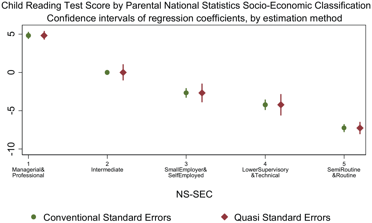
An example of the use of quasi-standard errors in an analysis of the UK Millennium Cohort Study.

A measure of highest parental National Statistics Socio-Economic Classification (NS-SEC) and a dummy variable for gender are included in the model. We are interested in interpreting the association between parental NS-SEC and reading test scores. Our reference category for parental NS-SEC is category 2 (Intermediate occupations) and using conventional standard errors (shown in green) we are able to compare the reading test performance of children in this category with those in the other NS-SEC categories. Using only conventional standard errors, we are not able to compare children in NS-SEC categories which do not include the reference category. For example, we are not able to compare children in NS-SEC category 3 (Small employers and own account workers) and those in NS-SEC category 4 (Lower supervisory and technical occupations). With the use of quasi-standard error based comparison intervals¹⁰ (shown in red), we are able to make comparisons between all possible combinations of NS-SEC categories. We can see, for example, that there are not significant differences between the reading test scores of children in NS-SEC categories 3 and 4, but there are significant differences between children in NS-SEC categories 3 and 5. Making comparisons across different categories in this way would not be possible if only regression coefficients and conventional standard errors were presented because a conventional error is not calculated for the reference category.

The example above illustrates the utility of estimating quasi-variance based measures. Reporting quasi-variance measures will increase the transparency of secondary data analyses. The facility to make additional comparisons is especially valuable when replicating analyses with other datasets and when undertaking reviews or meta-analyses where statistical models have been constructed with alternative parameterisations. Quasi-variance based statistics can now be routinely calculated as part of the statistical modelling process in both Stata and R, and results can conveniently be graphed. Therefore, we advocate that data analysts who are working with categorical explanatory variables routinely report quasi-variance based measures in their modelling results.

Parameter estimates in logistic regression models

Many data analysis modules within undergraduate and postgraduate sociology programmes introduce linear regression after bivariate correlations (and associated items such scatter plots). This is a pedagogically logical place in the curriculum to position this topic. Topics such as logistic regression will often be introduced on courses after linear regression. One example of this ordering is illustrated in the excellent instructional text by Marsh and Elliott (2008).

Linear regression models (often called multiple regression) are a reasonable starting point in learning about statistical models, but they are seldom used in applied sociological research. Even a cursory review of empirical analyses of social surveys reveals that logistic regression models are far more commonly used. Linear regression models are relatively uncommon in sociological research because there are so few social science outcome variables that are measured on metric scales. By contrast, there are an inordinate number of outcome variables that lend themselves to measurement on categorical scales. In particular, many social science outcome variables are discrete binary measures. These measures frequently take the form of ‘no’ or ‘yes’ or relate to the presence or absence of some condition. Logistic regression models are very commonly used in empirical analyses using large-scale social science datasets in disciplines such as sociology, social policy, politics and geography. By contrast, the probit model is ubiquitous within economic research. These models are simply special cases within the generalised linear model (GLM) framework¹¹ (Nelder and Wedderburn, 1972). Both are more complex compared with the linear regression model, and the complexities of these models are not always well understood by sociologists.

In this section, we provide a discussion of the complexities involved in presenting and interpreting the results of logistic regression models. Throughout this section, we illustrate these methodological points with a series of models estimated using data from the 1970 British Cohort Study.¹² Our example focuses on children’s performance on a maths test taken at around age 10 (in 1980). We have categorised performance on this test to 1 = above average scores and 0 = average and below average scores. Our explanatory variables are the seven category version of father’s NS-SEC, a binary variable indicating whether the child’s parents own their own home (1 = yes and 0 = no), and a binary variable of whether the child’s mother is rated as being very interested in her child’s education (1 = yes and 0 = no). In general, within regression models it is desirable that explanatory variables are not extremely highly correlated (i.e. collinear) (see Fox, 1991; Treiman, 2009: 108). In the current example, the three explanatory variables used have weak associations with each other and satisfy standard tests for multicollinearity.¹³

The effects of the individual explanatory variables in logistic regression models are far less intuitive than in a standard linear regression model. In the case of a linear regression model, the effect of a continuous explanatory variable can be interpreted in a relatively straightforward manner. This is because a one unit change in the explanatory variable leads to a change in the outcome variable equal to the value of the coefficient (the beta). There is not an equivalent simple interpretation of the effect of a single explanatory variable in a logistic regression model because estimation is undertaken using a transformation and results are presented on the log odds scale.

Table 1 reports the results of two statistical models. Model 1 is a linear regression of maths test scores and model 2 is a logistic regression of maths test scores categorised as 1 = above average and 0 = average and below. When interpreting the coefficients of the linear regression model, we can see that children whose fathers are in NS-SEC category 2 on average score 2.09 points lower than children with fathers in NS-SEC category 1, net of all other variables in the model.

Table 1.

An example of a linear regression model (model 1) and a logistic regression model (model 2). The outcome of model 1 is score on a maths test. The outcome of model 2 is the score on the same maths test categorised into above average (1) and average and below attainment (0).

		Model 1	Model 2
		Linear regression coefficients (standard errors)	Logistic regression coefficients log odds (standard errors)
Father’s NS-SEC	1. Large employers, higher managerial and professional	Ref.	Ref.
	2. Lower managerial and professional	−2.09^*** (0.50)	−0.30^** (0.10)
	3. Intermediate	−2.52^*** (0.55)	−0.34^** (0.11)
	4. Small employers and own account workers	−4.38^*** (0.52)	−0.67^*** (0.10)
	5. Lower supervisory and technical	−5.34^*** (0.48)	−0.82^*** (0.09)
	6. Semi-routine	−5.77^*** (0.50)	−0.89^*** (0.10)
	7. Routine	−6.80^*** (0.49)	−0.95^*** (0.09)
Home owner		3.53^*** (0.27)	0.53^*** (0.05)
Mother very interested in child’s education		5.29^*** (0.26)	0.74^*** (0.05)
Constant		44.19 (0.46)	0.01 (0.09)
Adjusted R²		0.15
McFadden’s adjusted R²			0.07
McKelvey and Zavoina’s R²			0.13
Cragg and Uhler’s R²			0.13
n		8198	8198

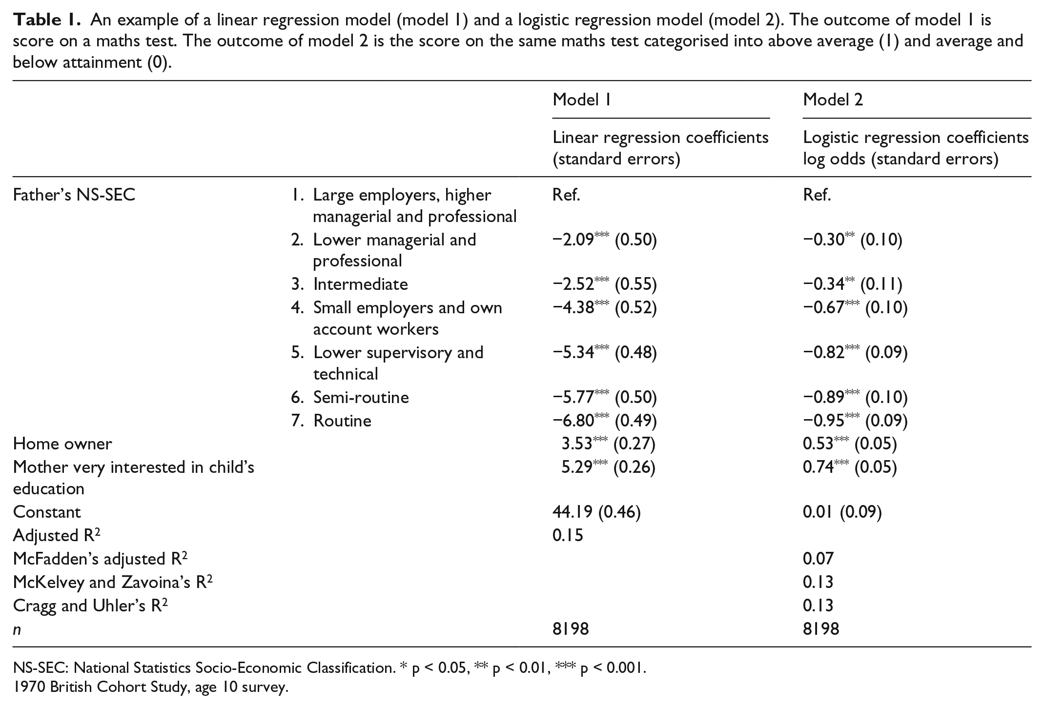
NS-SEC: National Statistics Socio-Economic Classification. * p < 0.05, ** p < 0.01, *** p < 0.001.

1970 British Cohort Study, age 10 survey.

The interpretation of model 2 is less straightforward. In statistical terms, children whose fathers are in NS-SEC category 2 have a decreased log odds of 0.30 of achieving an above average score on the maths test, compared with children who have fathers in NS-SEC category 1, net of all other variables in the model. Although this tells us that the more advantaged children in NS-SEC category 1 perform better on the maths test. In our experience, many sociologists find that the further interpretation of log odds is far from intuitive.

Odds ratios

There are several alternative ways in which the results of a logistic regression model can be presented, which we illustrate in Table 2. The use of odds ratios is frequently advocated (see Rubin, 2012; Tolmie et al., 2011). Odds ratios are calculated by exponentiating estimates of log odds for the explanatory variables. In model 2, the odds of getting an above average score on the maths test is 0.74 for children whose fathers are in NS-SEC category 2 compared with children who have fathers in NS-SEC category 1, net of other variables in the model.

Table 2.

An example of the different presentation of parameter estimates from a logistic regression model of maths test scores (model 2 in Table 1).

Father’s NS-SEC	1	2	3	4	5
Father’s NS-SEC	Log odds	Odds ratio	Gelman and Hill (probability)	Conditional marginal effects (probability)	Adjusted prediction (probability)
1. Large employers, higher managerial and professional	Ref.	Ref.	Ref.	Ref.	0.67
2. Lower managerial and professional	−0.30^**	0.74^**	−0.08^**	−0.07^**	0.60
3. Intermediate	−0.34^**	0.71^**	−0.09^**	−0.08^**	0.59
4. Small employers and own account workers	−0.67^***	0.51^***	−0.17^***	−0.16^***	0.51
5. Lower supervisory and technical	−0.82^***	0.44^***	−0.21^***	−0.20^***	0.47
6. Semi-routine	−0.89^***	0.41^***	−0.22^***	−0.21^***	0.46
7. Routine	−0.95^***	0.39^***	−0.24^***	−0.23^***	0.44

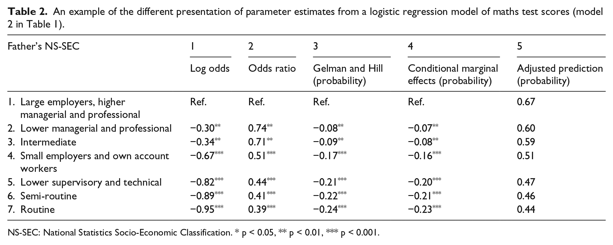
NS-SEC: National Statistics Socio-Economic Classification. * p < 0.05, ** p < 0.01, *** p < 0.001.

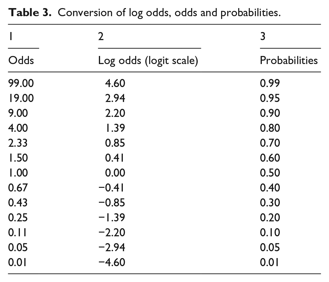
Odds ratios are a convenient means of understanding the effects of explanatory variables in logistic regression models. A hidden consequence of converting coefficients measured on the log odds scale to odds ratios is that the transformation is not linear. In our experience, this is not widely appreciated by sociological researchers. Table 3 illustrates that log odds from −4.60 to 0 (column 2) are transformed into odds from 0.01 to 1.00 (column 1). By contrast, log odds from 0 to +4.60 (column 2) are transformed into odds from 1.00 to 99.00 (column 1). Therefore, some caution should be applied when using odds ratios to communicate the effects of explanatory variables in logistic regression models. Some researchers present odds ratios in graphical formats to aid interpretation. When odds ratios that are both greater and less than 1 are simultaneously presented, the non-linear nature of odds ratios will be visually misleading. It is worth noting that while log odds map onto odds asymmetrically, they map on to probabilities symmetrically (see Table 3 column 3). Therefore, we conclude that in general presenting coefficients as log odds values is usually more appropriate than presenting them as odds ratios.

Table 3.

Conversion of log odds, odds and probabilities.

1	2	3
Odds	Log odds (logit scale)	Probabilities
99.00	4.60	0.99
19.00	2.94	0.95
9.00	2.20	0.90
4.00	1.39	0.80
2.33	0.85	0.70
1.50	0.41	0.60
1.00	0.00	0.50
0.67	−0.41	0.40
0.43	−0.85	0.30
0.25	−1.39	0.20
0.11	−2.20	0.10
0.05	−2.94	0.05
0.01	−4.60	0.01

Gelman and Hill (2008) suggest that as a rule of convenience, analysts should take logistic regression coefficients (other than the constant term) and divide them by 4 to get an upper bound of the predictive difference corresponding to a one unit change in the explanatory variable. We illustrate this approach in column 3 of Table 2. The log odds reported in column 1 of Table 2 are divided by 4. Although this technique is not widely known, it appears to provide a quick and easy substantive interpretation of estimates reported on a log odds scale.¹⁴

Marginal effects

The use of marginal effects to interpret statistical models is well known in economics (see Greene, 2008), but less known in other social science disciplines. Expressed simply, marginal effects are statistics that are presented to aid the interpretation of modelling results. They are calculated from a regression model at fixed values of some explanatory variables and/or averages of other explanatory variables (for extended discussion, see Long and Freese, 2006; Williams, 2012).¹⁵

We depict two examples of marginal effects. The first are usually known as conditional marginal effects (a terminology used in Stata output). In Table 2 column 4, we present conditional marginal effects (reported as probabilities) for the father’s NS-SEC variable. The marginal effects are calculated with the other explanatory variables held at their mean. For example, a child whose parents are from NS-SEC 2 and who has average characteristics on the other explanatory variables will on average have a probability of obtaining an above average maths test score of 0.08 lower than a counterpart with parents from NS-SEC 1. This specific form of description relates to ‘average characteristics’ on the other explanatory variables.¹⁶ We conclude that using marginal effects provides a convenient and interpretable method of reporting the effects of an explanatory variable in logistic regression analyses.

The conditional marginal effects presented in Table 2 are estimated when the other explanatory variables are held at their means, but it is also possible to calculate marginal effects when the other variables are fixed at substantively meaningful levels. One of the authors has positive direct experience of communicating results from logistic regression models to civil servants using marginal effects at representative values (see Gayle et al., 2003).

A second form of marginal effect is known as ‘adjusted predictions’.¹⁷ These measures show probabilities of the outcome, for a level of the explanatory variable with the other explanatory variables set at a specified level (e.g. their means). We report the adjusted predictions for model 2 in Table 2 column 5. The adjusted predictions are readily interpretable because they are probabilities. For example, the predicted probability of a child getting an above average score is 0.67 for the children with fathers in NS-SEC category 1 (with other explanatory variables at their average values). By contrast, the predicted probability of a child getting an above average score is 0.44 for the children with fathers in the lowest NS-SEC category (with other variables set at their averages). At the time of writing, marginal effects are seldom reported outside of economics where they are widely used. We concur with Angrist and Pischke (2008) that output from non-linear models (such as the logit model) are much more interpretable when marginal effects are reported.

Sample enumeration

Although not widely used, another useful alternative way to represent the results of logistic regression models is sample enumeration (see Davies, 1992; Gayle et al., 2002). This method operates in a similar fashion to marginal and predicted probabilities but is essentially derived from within the sample rather than using means or specific values to illustrate the effects of other explanatory variables in the model. Sample enumeration allows researchers to quantify the substantive importance of statistically significant explanatory variables in a logistic regression model. The use of measures such as odds ratios does not immediately address the issue of how much of the observed relationship is explained by one variable in the model (e.g. father’s NS-SEC) compared to how much is explained by the other explanatory variables in the model.

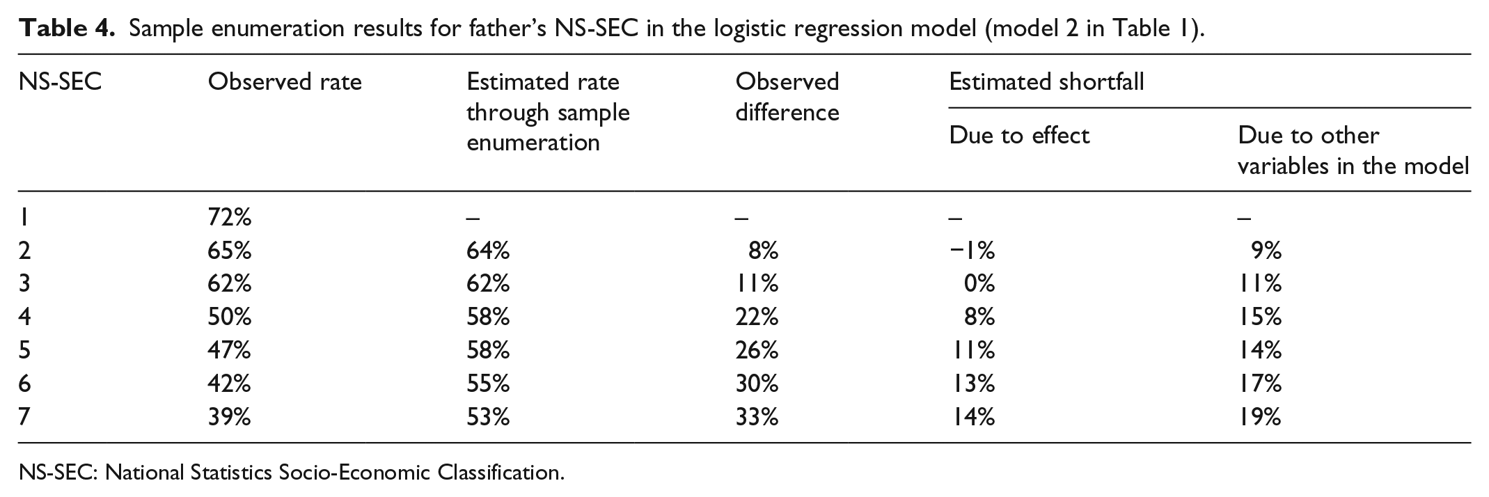
In the present example, the sample enumeration approach allows us to ask the question,

what percentage of children in the least advantaged NS-SEC category would have achieved an above average score on the maths test if they had been in the most advantaged category, given their other characteristics which are measured by other variables included in the model?

Through sample enumeration, we hypothetically move all of the children in the least advantaged NS-SEC category to the most advantaged category. Using the logistic regression model results, we can then estimate the proportion of these children who would have achieved an above average test score given their other characteristics (measured by the other explanatory variables included in the model).

A detailed example of the sample enumeration process is given in Gayle et al. (2002). In our present example, sample enumeration first involves extracting children from the least advantaged NS-SEC category in the sample. Results from the full logistic regression model (with all cases included) are then used to predict the outcome for each child in the least advantaged NS-SEC category, but with the NS-SEC effect set to zero. This is analogous to promoting each child in the least advantaged NS-SEC category to the most advantaged category. This allows us to estimate the probability of each of these children gaining an above average test score if they were moved into the most advantaged NS-SEC, but with their other characteristics remaining exactly the same. Summing these individual predicted probabilities allows us to construct expected frequencies (and therefore expected proportions) of children achieving an above average test score having eliminated the direct effect of NS-SEC.

The results of the sample enumeration are reported in Table 4. They show that 39% of those in the least advantaged NS-SEC category attained an above average maths test score (the observed rate). The sample enumeration rate is 53%, and this figure can be interpreted as the percentage of children in the least advantaged NS-SEC category that would have achieved an above average score on the maths test if they had been in the most advantaged category, given their other characteristics which are measured by other variables included in the model.¹⁸ The sample enumeration method has isolated the direct effect of NS-SEC, 14% in this case. The observed or ‘original’ difference between the rates of children attaining an above average test score in the most advantaged NS-SEC and in the least advantaged NS-SEC was 33% (72%–39%). This figure is the observed difference or ‘shortfall’ between the rates of attainment of above average scores in these two groups. Through sample enumeration, we are able to report that 14% of the original 33% shortfall is due to the effect of NS-SEC. We can therefore conclude that 19% of the original shortfall is due to the combined effects of the other explanatory variables in the model.

Table 4.

Sample enumeration results for father’s NS-SEC in the logistic regression model (model 2 in Table 1).

NS-SEC	Observed rate	Estimated rate through sample enumeration	Observed difference	Estimated shortfall
NS-SEC	Observed rate	Estimated rate through sample enumeration	Observed difference	Due to effect	Due to other variables in the model
1	72%	–	–	–	–
2	65%	64%	8%	−1%	9%
3	62%	62%	11%	0%	11%
4	50%	58%	22%	8%	15%
5	47%	58%	26%	11%	14%
6	42%	55%	30%	13%	17%
7	39%	53%	33%	14%	19%

NS-SEC: National Statistics Socio-Economic Classification.

Although the sample enumeration approach has not been widely used in sociological research, we are convinced that it provides an attractive means of quantifying the substantive importance of the effect of key variables in a form that may be relatively easily understood. We also suspect that this approach might be useful when communicating logistic regression results to researchers and other stakeholders whose interests may be substantive but who may not have an especially sophisticated understanding of concepts such as log odds or odds ratios.

The presentation of logistic regression results

There are no strict protocols for presenting the results of statistical models, and there is a large amount of variation between the formats used in academic publications. From the discussions provided above, we can make several suggestions on reporting information from logistic regression models. Log odds (i.e. coefficients) should be presented as this information conveys both the direction and the size of the effect. Conventional standard errors should be reported as they indicate the precision of the effect. In combination with coefficients, the reporting of standard errors allows readers to formally assess significance and makes other statistics such as p values and z values redundant. Some researchers might be uncomfortable with the suggestion that p values are not required and as a compromise they might choose to also include asterisks (*) to indicate levels of significance.

We strongly advocate reporting quasi-variance based standard errors because these measures facilitate the calculation of comparison intervals and therefore address the reference category problem. Table 5 illustrates a format where there is sufficient space to report both quasi-variance standard errors and comparison intervals. We also consider that conditional marginal effects (probabilities) should routinely be reported as this greatly aids the interpretation of the effects of explanatory variables. We consider that there is additional benefit in reporting the lower and upper bounds of this measure.

Table 5.

An example of the ideal presentation of a logit model.

		Log odds	SE	QV SE	QV SE CI		Conditional marginal effects (probability)	Conditional marginal effects (95% CI)
		Log odds	SE	QV SE	Lower	Upper	Conditional marginal effects (probability)	Lower	Upper
Father’s NS-SEC	1. Large employers, higher managerial and professional	Ref.	–	0.00	−0.18	0.18	–	–	–
	2. Lower managerial and professional	−0.30^**	(0.10)	0.10	−0.45	−0.15	−0.07^**	−0.11	−0.02
	3. Intermediate	−0.34^**	(0.11)	0.11	−0.52	−0.17	−0.08^**	−0.13	−0.03
	4. Small employers and own account workers	−0.67^***	(0.10)	0.10	−0.82	−0.52	−0.16^***	−0.21	−0.12
	5. Lower supervisory and technical	−0.82^***	(0.09)	0.09	−0.95	−0.70	−0.20^***	−0.24	−0.16
	6. Semi-routine	−0.89^***	(0.10)	0.10	−1.02	−0.75	−0.21^***	−0.26	−0.17
	7. Routine	−0.95^***	(0.09)	0.09	−1.07	−0.83	−0.23^***	−0.27	−0.19
Home owner		0.53^***	(0.05)	–	–	–	0.13^***	0.11	0.16
Mother very interested in child’s education		0.74^***	(0.05)	–	–	–	0.19^***	0.16	0.21
Constant		0.01	(0.09)	–	–	–	–	–	–
n		8198
McFadden’s adjusted R²		0.07
McKelvey and Zavoina’s R²		0.13
Cragg and Uhler’s R²		0.13
BIC null model		11,364
BIC full model		10,574

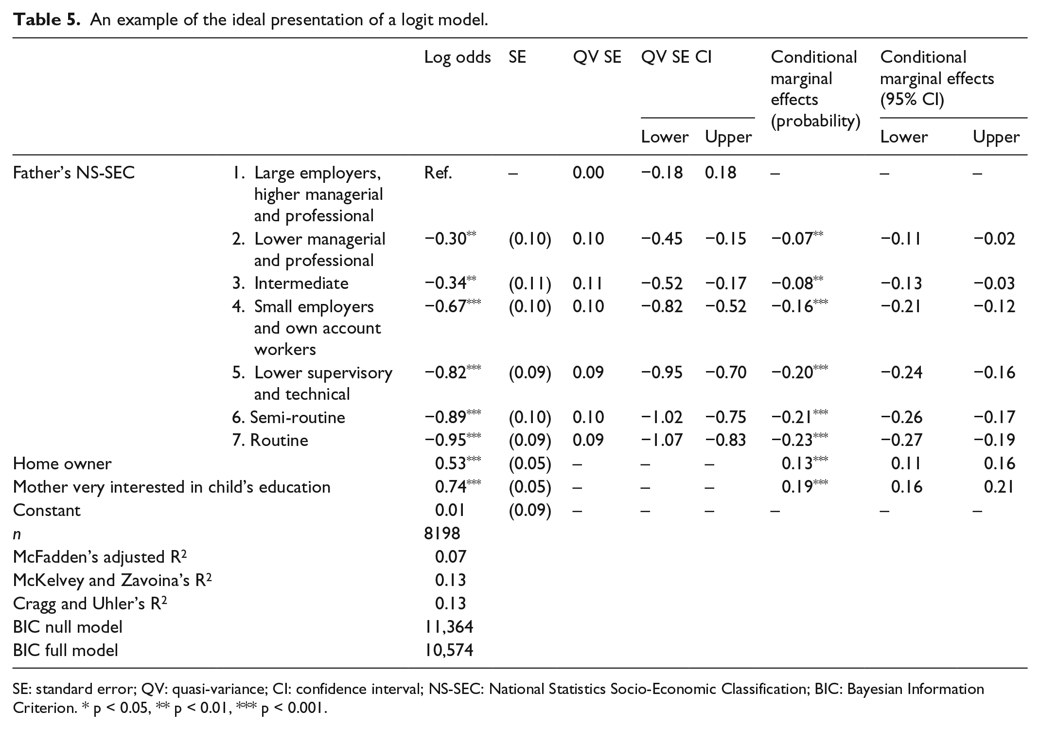
SE: standard error; QV: quasi-variance; CI: confidence interval; NS-SEC: National Statistics Socio-Economic Classification; BIC: Bayesian Information Criterion. * p < 0.05, ** p < 0.01, *** p < 0.001.

In addition to these statistical measures, it is always good practice for data analysts to report sample sizes (n) and model fit statistics. Smithson (2003) pithily remarks that there has been something of a cottage industry in model fit statistics for logistic regression. Long and Freese (2006) provide an excellent overview of the scope and limitations of these measures. Software packages such as Stata report a wide range of pseudo R² measures.¹⁹ We are not persuaded that any single pseudo R² should be routinely preferred above all others. At the current time, we suggest that researchers should report a few alternative measures in published research but provide as many pseudo R² measures as practicable in the documentation of their workflow. When comparing nested models, there is a compelling case for using a measure that accounts for parsimony such as the Bayesian Information Criterion (BIC)²⁰ which was proposed by Raftery (1986).

Comparing nested models

It is often useful to present results as a series of nested models. Looking again at the example of children’s scores on the maths test, we may first seek to examine the association between father’s NS-SEC and whether a child attained an above average test score. We may then seek to investigate the extent of the effect of father’s NS-SEC when other factors are also included in the model (e.g. parental home ownership and maternal interest in the child’s education, see Table 6).

Table 6.

An example of a series of logistic regression models. The outcome is score on the same maths test categorised to above average (1) and average and below attainment (0).

		Model 1 Log odds (SE)	Model 2 Log odds (SE)	Model 3 Log odds (SE)
Father’s NS-SEC	1. Large employers, higher managerial and professional	Ref.	Ref.	Ref.
	2. Lower managerial and professional	−0.36^*** (0.10)	−0.30^** (0.10)	−0.30^** (0.10)
	3. Intermediate	−0.49^*** (0.11)	−0.37^*** (0.11)	−0.34^** (0.11)
	4. Small employers and own account workers	−0.97^*** (0.10)	−0.78^*** (0.10)	−0.67^*** (0.10)
	5. Lower supervisory and technical	−1.10^*** (0.09)	−0.93^*** (0.09)	−0.82^*** (0.09)
	6. Semi-routine	−1.27^*** (0.09)	−1.02^*** (0.10)	−0.89^*** (0.10)
	7. Routine	−1.41^*** (0.09)	−1.11^*** (0.09)	−0.95^*** (0.09)
Home owner			0.66^*** (0.05)	0.53^*** (0.05)
Mother very interested in child’s education				0.74^*** (0.05)
Constant		0.97 (0.07)	0.41 (0.09)	0.01 (0.09)
McFadden’s adjusted R²		0.04	0.05	0.07
McKelvey and Zavoina’s R²		0.06	0.09	0.13
Cragg and Uhler’s R²		0.07	0.10	0.13
n		8198	8198	8198

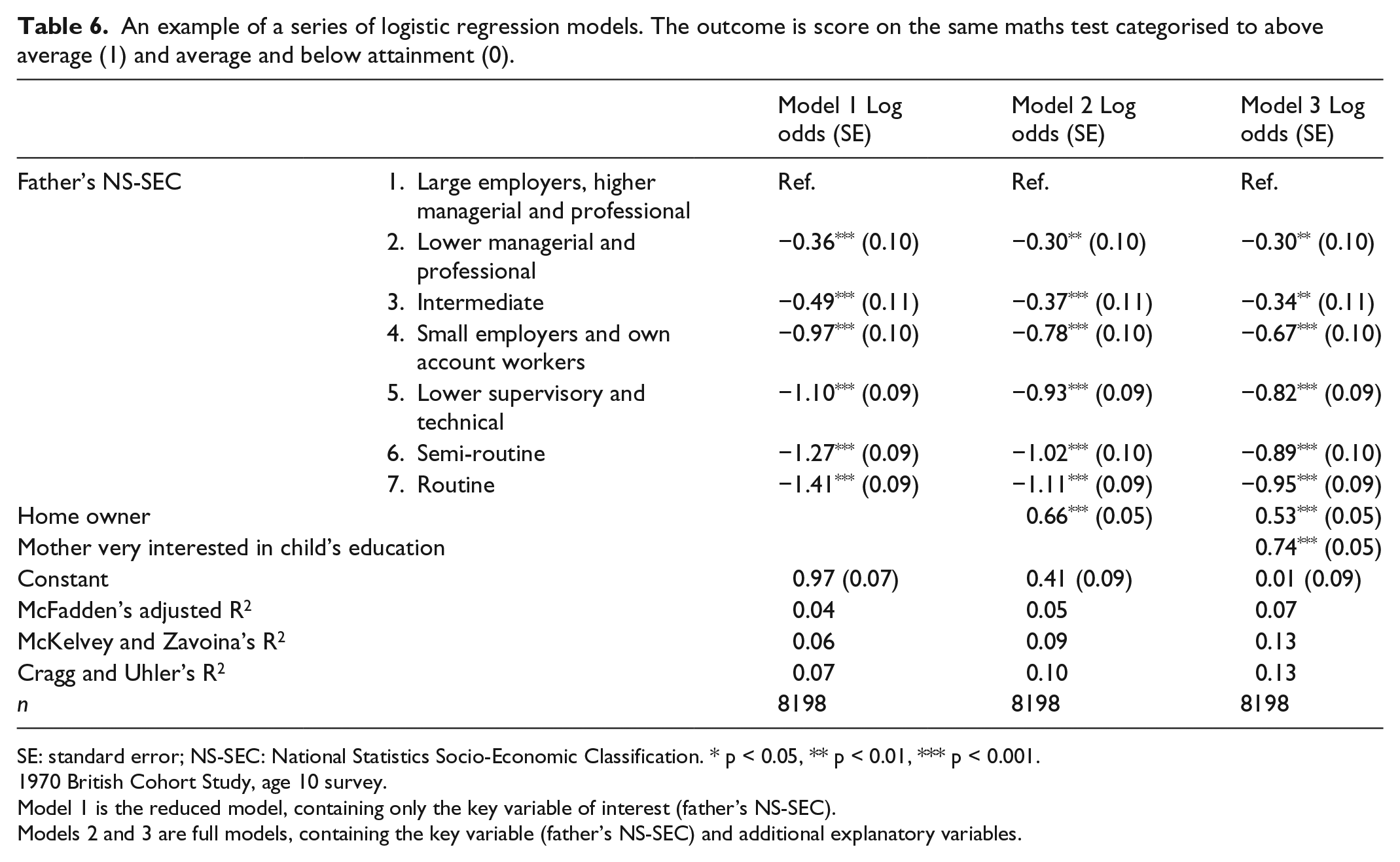
SE: standard error; NS-SEC: National Statistics Socio-Economic Classification. * p < 0.05, ** p < 0.01, *** p < 0.001.

1970 British Cohort Study, age 10 survey.

Model 1 is the reduced model, containing only the key variable of interest (father’s NS-SEC).

Models 2 and 3 are full models, containing the key variable (father’s NS-SEC) and additional explanatory variables.

The comparison of coefficients in nested models is relatively straightforward when analysing linear outcome variables. If a coefficient of one explanatory variable is observed to decline after another explanatory variable is added to the model, this has the convenient interpretation that its effect on the outcome variable is not as substantial once the new variable has been included in the analysis. Unfortunately, the interpretation is not so straightforward for non-linear models, a point that is not widely understood (for extended discussion, see Mood, 2010). This issue arises because non-linear models have what is known as a fixed variance (the fixed variance in the logit model is π² / 3). Adding variables to the model can change the estimated coefficients, even when the explanatory variables are not related. This means that for nested non-linear models, the size of coefficients for the same variables may differ simply because of the rescaling of the model that arises when additional variables are added and should not be given a simple substantive interpretation (Kohler et al., 2011).

When examining the series of nested logistic models presented in Table 6, we may naively interpret the reduction in the log odds for the least advantaged NS-SEC category as evidence that part of the this effect has been explained by the additional variables that have been added to the model. We are unable to conclude this from the details presented in Table 6, however. This is because the changes in the log odds observed may be the result of the rescaling of the model rather than a genuine substantive effect.

Several different solutions have been proposed to deal with the problem of comparing coefficients across nested non-linear models (see Erikson et al., 2005; Winship and Mare, 1984; Wooldridge, 2010). Karlson et al. (2012) and Breen et al. (2013) demonstrate that previous approaches to this problem are suboptimal and they have developed the Karlson–Holm–Breen (KHB) method as a more effective solution. This technique can be implemented through the -khb- program in Stata (see Kohler et al., 2011). KHB estimates the changes in the coefficients of a logit model that are the result of rescaling when new variables are introduced to the model. This allows the analyst to determine the total effect of a variable (e.g. NS-SEC in the example above) into direct effects and indirect effects.

Table 7 presents the results of the KHB technique applied to our example. As in Table 6, model 2 contains father’s NS-SEC and home ownership, and model 3 contains NS-SEC, home ownership and mother’s interest in the child’s education. The KHB method allows us to interpret the effect of a key variable, in this case father’s NS-SEC, taking into account the effects of rescaling.

Table 7.

An example of the use of the KHB method to interpret the effect of father’s NS-SEC in a series of nested logistic regression models. The outcome is score on the same maths test categorised to above average (1) and average and below attainment (0).

		Model 2		Model 3
		Log odds	SE	Log odds	SE
1. Large employers, higher managerial and professional	Reduced	Ref.		Ref.
	Full
	Difference
2. Lower managerial and professional	Reduced	−0.36^***	(0.10)	−0.37^***	(0.10)
	Full	−0.30^**	(0.10)	−0.30^**	(0.10)
	Difference	−0.06^*	(0.03)	−0.07	(0.05)
3. Intermediate	Reduced	−0.49^***	(0.11)	−0.50^***	(0.11)
	Full	−0.37^***	(0.11)	−0.34^**	(0.11)
	Difference	−0.11^***	(0.03)	−0.15^**	(0.05)
4. Small employers and own account workers	Reduced	−0.98^***	(0.10)	−1.00^***	(0.10)
	Full	−0.78^***	(0.10)	−0.67^***	(0.10)
	Difference	−0.20^***	(0.03)	−0.33^***	(0.05)
5. Lower supervisory and technical	Reduced	−1.11^***	(0.09)	−1.14^***	(0.09)
	Full	−0.93^***	(0.09)	−0.82^***	(0.09)
	Difference	−0.18^***	(0.03)	−0.32^***	(0.05)
6. Semi-routine	Reduced	−1.29^***	(0.09)	−1.32^***	(0.10)
	Full	−1.02^***	(0.10)	−0.89^***	(0.10)
	Difference	−0.27^***	(0.04)	−0.43^***	(0.05)
7. Routine	Reduced	−1.43^***	(0.09)	−1.46^***	(0.09)
	Full	−1.11^***	(0.09)	−0.95^***	(0.09)
	Difference	−0.31^***	(0.04)	−0.51^***	(0.05)

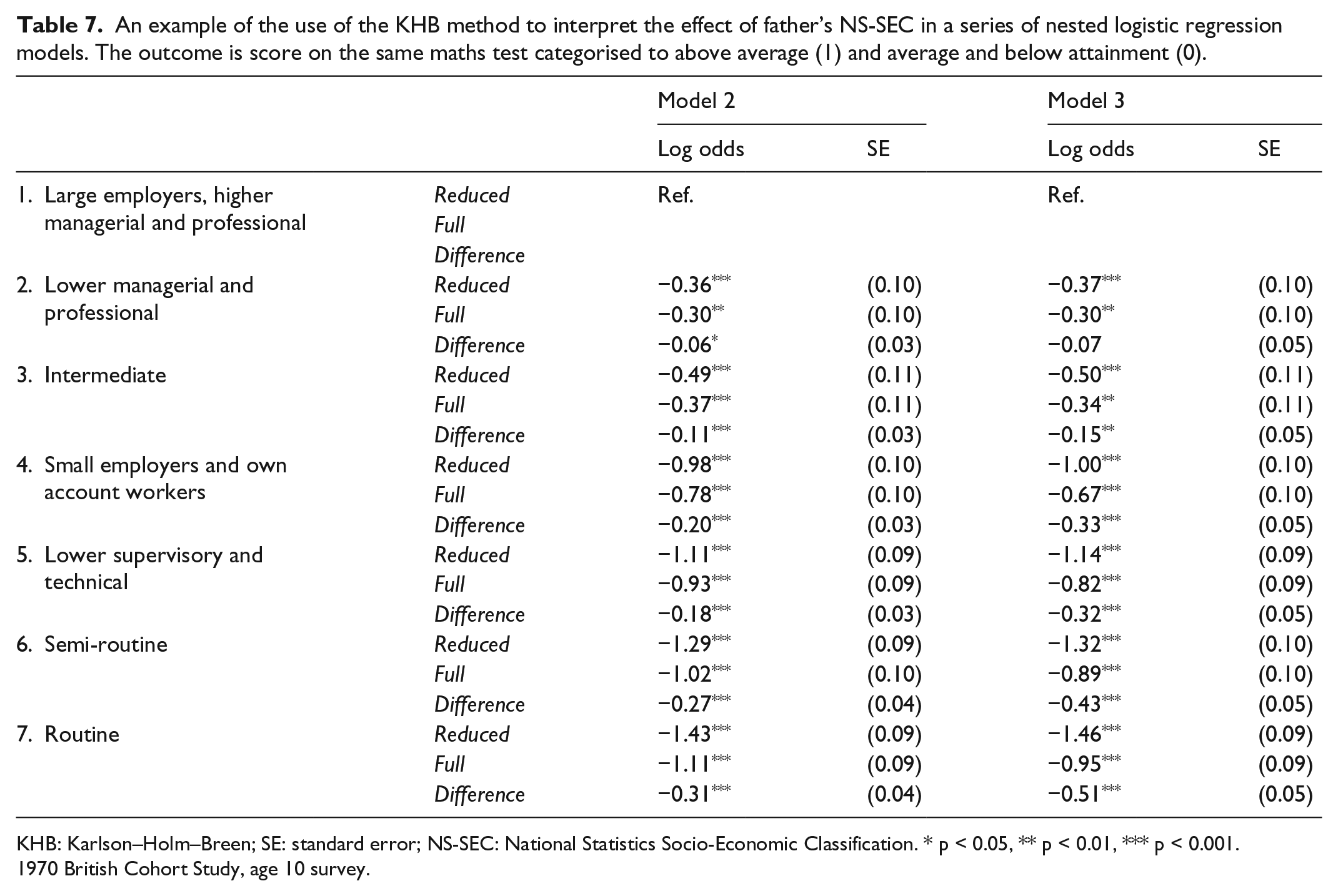
KHB: Karlson–Holm–Breen; SE: standard error; NS-SEC: National Statistics Socio-Economic Classification. * p < 0.05, ** p < 0.01, *** p < 0.001.

1970 British Cohort Study, age 10 survey.

Table 7 shows the estimated effect of father’s NS-SEC in the reduced model (e.g. model 1 in Table 6), the estimated effects in the full model (e.g. model 2 in Table 6) and the difference between the effect of father’s NS-SEC in these two models. The estimated effect of the key variable on the outcome variable is called the direct effect (see Figure 2). When we add additional explanatory variables to the model, some of this direct effect may be accounted for by these additional variables, this is called the indirect effect (see Figure 3). In Figure 3, the direct effect of father’s NS-SEC may be partly explained by the inclusion of parental home ownership, or due to rescaling. Using only conventional logistic regression results, we are unable to determine whether the direct effect of father’s NS-SEC may be partly explained by the inclusion of parental home ownership, or due to rescaling. The crux of the KHB method is to ensure that the estimated indirect and direct effects are better understood and can be given more substantively meaningful interpretations.

Figure 2.

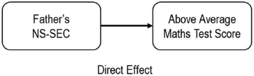
The effect of father’s NS-SEC in the reduced model (Table 6, model 1).

Figure 3.

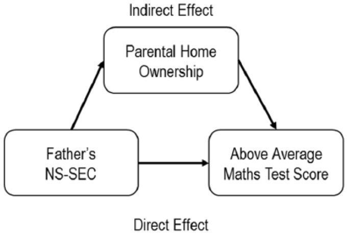
The effect of father’s NS-SEC and parental home ownership in the full model (Table 6, model 2).

We can see from Table 7 model 3 that the log odds of gaining an above average score are decreased by 0.37 for children with fathers in NS-SEC category 2 compared to those in the reference category (NS-SEC category 1). Controlling for home ownership and mother’s interest in the child’s education, the direct effect of being in the most advantaged NS-SEC category is reduced to 0.30, leaving an indirect effect of 0.07. To aid in the interpretation of these effects, Karlson et al. (2012) suggest reporting three measures, the confounding ratio, confounding percentage and the rescaling factor (shown in Table 8).

Table 8.

Confounding ratio and confounding percentage from the KHB method to interpret the effect of father’s NS-SEC in a series of nested logistic regression models. The outcome is score on the same maths test categorised to above average (1) and average and below attainment (0).

	Model 2			Model 3
	Confounding ratio	Confounding percentage	Rescaling factor	Confounding ratio	Confounding percentage	Rescaling factor
1. Large employers, higher managerial and professional	Ref.	Ref.	Ref.	Ref.	Ref.	Ref.
2. Lower managerial and professional	1.20	17	1.00	1.23	19	1.03
3. Intermediate	1.31	23	1.00	1.45	31	1.02
4. Small employers and own account workers	1.25	20	1.01	1.49	33	1.03
5. Lower supervisory and technical	1.20	17	1.01	1.38	28	1.04
6. Semi-routine	1.26	21	1.01	1.49	33	1.04
7. Routine	1.28	22	1.01	1.53	35	1.04

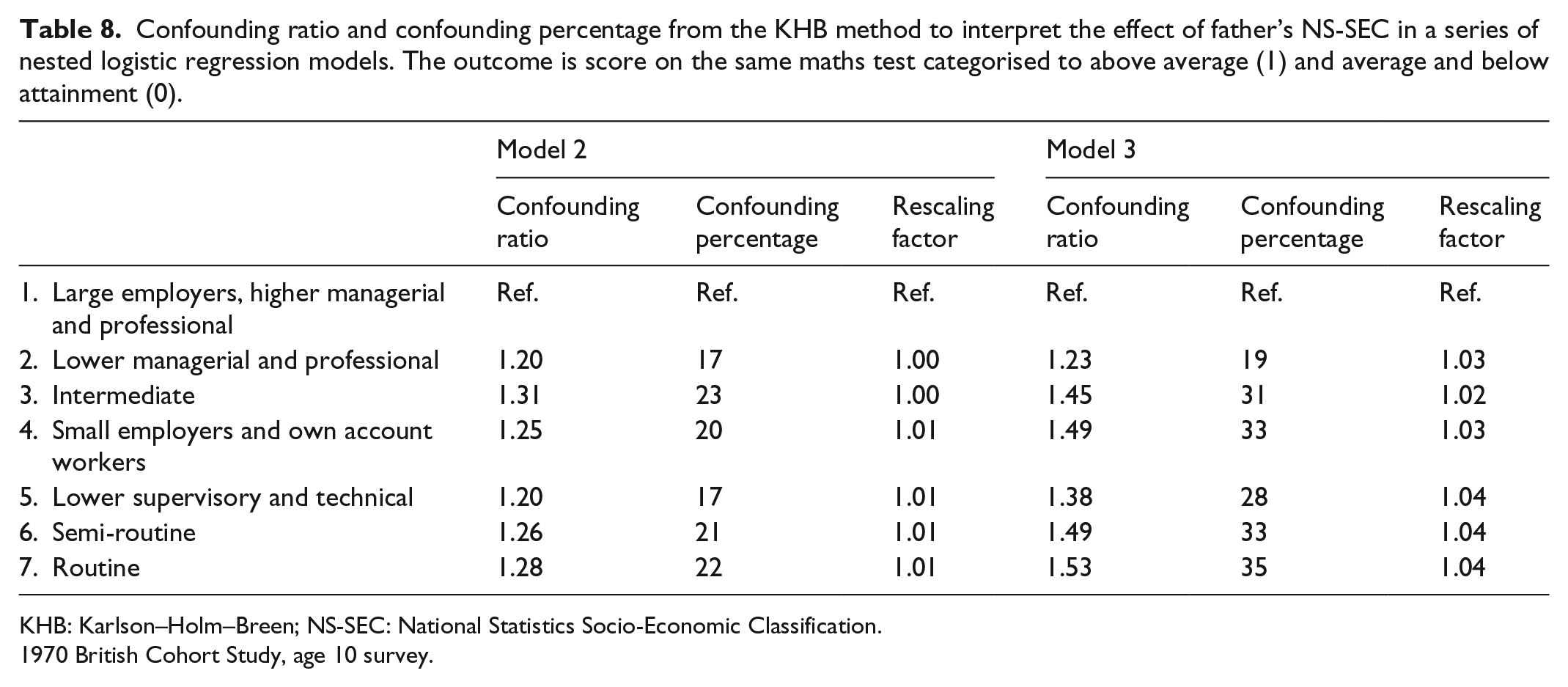
KHB: Karlson–Holm–Breen; NS-SEC: National Statistics Socio-Economic Classification.

1970 British Cohort Study, age 10 survey.

The confounding ratio for model 3 indicates that the total effect (i.e. the sum of the direct and indirect effects) for the NS-SEC category 2 is 1.23 times larger than the direct effect (i.e. the effect of NS-SEC that remains after controlling for the additional variables). The confounding percentage for model 3 indicates that 19% of the total effects of being in NS-SEC category 2 is due to the additional explanatory variables added to the model. Iannelli (2013) neatly demonstrates an application of the KHB method, and the use of the confounding percentage, in her analysis of the National Child Development Study. In order to investigate the extent to which school type and school curricula mediate the effect of social background factors on entry to the service class, she utilises the KHB method to compare the coefficients of origin, social class and parental education across a series of models. She concludes that taken together, school type and curricula can provide an additional advantage in the process of social mobility (Iannelli, 2013). We envisage that the KHB approach is especially attractive in studies where researchers are interested in understanding the effects of mediating variables. There are many examples of this in social stratification research which follows from the classic work of Blau and Duncan (1967). Although the KHB technique is relatively new, there are a growing number of social science studies which utilise this method (e.g. see Gabay-Egozi et al., 2015; Gracia et al., 2013; Iannelli, 2013; Pais, 2014; Whelan and Maître, 2014).

Non-linear associations

In some secondary data analyses, the association between an explanatory variable and a dependent variable is non-linear. Treiman (2009) highlights the example of the association between age and income because in many countries (e.g. the United States) income generally increases with age up to a certain point and then begins to fall. Non-linear relationships between explanatory and dependent variables provide interpretational challenges in simple regression models. Fortunately, there is a straightforward solution to this problem, because the analyst can operationalise suitable transformations of the independent variables.

Within sociological research, transformations are sometimes appropriate, such as power transformations (i.e. squaring or cubing the variable), or using a log transformation (see Treiman, 2009: 140–145). In some cases, the relationships between variables are highly complex and not captured with simpler variable transformations. In such scenarios, analysts could consider the use of a spline function. The use of splines results in a series of linear or curvilinear associations, with points of disjuncture (i.e. knots) where the degree of association is changed (see Marsh and Cormier, 2002). Splines can be implemented quite easily with conventional software (i.e. using dummy variables and polynomial expressions), although in some empirical circumstances extended thought will be required when interpreting results.

There are very many situations in sociological analysis when the use of non-linear transformations makes for a useful explanation of observed patterns of association (Treiman, 2009). In particular, in the case of exploring trends through time with educational and/or occupational measures, it is plausible that the relationship follows some form of non-linear or step relationship, which can be captured by a non-linear transformation. Such relationships would be described sub-optimally if this was not represented in the analysis. For example, the use of non-linear transformations in the analysis of educational inequality over time in the Netherlands is demonstrated by Buis (2009). The downside of the use of non-linear transformations is that they can be very difficult to interpret substantively. We suggest that this may be aided by the use of graphical or visual representation of modelling results.

Intersectionality and interaction effects

When modelling the effects of multiple explanatory variables, it is important to remember that influences can be separated between those that are independent of the values of other explanatory variables (i.e. ‘main effects’), and those that are conditional upon values of other explanatory factors (i.e. ‘interaction effects’) (see Dubrow, 2008; Steinbugler and Dias, 2006; Treiman, 2009; Warner, 2008). In particular, the total influence of a given explanatory factor is best understood as the combination of its main effect and that of any relevant interaction effects. Interaction effects can generally be interpreted as the distinctive outcome associated on average with being in a certain combination of circumstances across the various relevant factors. Statistical interaction effects are very similar in character to the concept of ‘intersectionality’ that is widely used to describe the interplay between different dimensions of difference in people’s lives (e.g. Platt, 2011; see also Davis, 2008).

Examining the interactions between variables that identify multiple characteristics of individuals (e.g. their gender, ethnicity and social class) is a methodological strategy for examining intersectionality. Strand (2014) provides a demonstration of the examination of intersectionality using interaction effects. He notes that analysts generally investigate main effects when studying educational inequalities but that it may be misleading to consider these main effects in isolation. He investigates the effects of the combination of ethnicity, social class and gender on General Certificate of Secondary Education (GCSE) attainment using the Longitudinal Study of Young People in England.²¹ He finds a complex picture of interactions between these variables and emphasises, in particular, the low attainment of White children from low social class groups. Strand’s (2014) results highlight the additional insights which can be gained by explicitly attempting to explore intersectionality by including interaction effects within statistical models.

Models can be estimated that include numerous interaction terms, and higher-order interactions are possible. Hypothetically, a ‘saturated’ model could be estimated that included all possible interaction effects between explanatory variables (including higher-order interactions). A potentially useful model fit statistic could be based on the difference between the saturated model and a current substantive model. In sociological applications where numerous explanatory variables are often relevant, fitting saturated models is seldom practicable because these models are unwieldy and they are often impossible to estimate with desktop computers and standard software packages. Data analysts generally recognise a trade-off between parsimony and interpretability when considering interaction terms, and for this reason it is commonly considered good practice to introduce interaction terms sparingly within the model building process.

Consider a model which included a seven category measure of NS-SEC and a two category measure of gender as explanatory variables. An interaction effect between these two explanatory variables will require six extra parameters. As the number of categories in each explanatory variable increases, effects become very difficult to interpret. Multi-way interactions are often also hard to replicate and sometimes tricky to compare across studies. One recommendation, highlighted in the previous papers in this special section, is that the use of metric (i.e. scale) rather than categorical variables greatly improves the parsimony of interaction effects and their ease of interpretation.

Analysts may also consider modelling categorical differences related to key variables through more advanced Generalised Linear Mixed Models (GLMM). Gelman and Hill (2007) suggest comparing the comparative aspects of different groupings of a categorical explanatory variable by estimating models that partition the variance of the outcome across levels of the explanatory variable (e.g. for each category of an occupation based socioeconomic variable). This is achieved by estimating a random effects model where the random effect represents levels of the observed explanatory variable. This strategy is not routinely employed in social research, but we can foresee situations where this could prove insightful, particularly for measures of variables where there are potentially a lot of different categories such as occupations. Once again, we envisage that this form of exploratory activity could also suitably be reported as a component of a more extensive sensitivity analysis; even if it did not form part of a published output, it should be made accessible for example in a data supplement.

Sensitivity analysis

With a large number of possible forms of key variables measuring occupation, education and ethnicity, it may seem like a daunting task to select the correct measure for an analysis. As we have stressed in the previous papers in this special section, a sensible and defensible solution is to explore several different operationalisations of the key variable. We have repeatedly suggested that operationalising a measure of occupation, education or ethnicity is not a simple case of selecting one superlative measure, and there may be many plausible candidate measures. The alternatives also might often have different functional forms (e.g. categories vs scaling). We recommend that secondary data analysts should routinely undertake sensitivity analyses that compare and evaluate the performance of alternative measures within the statistical models that they are developing.

Sensitivity analysis is the umbrella term for the investigative process of evaluating different analyses, for example, alternative statistical models. This involves investigating the influence which changes in a model (e.g. the use of different operationalisations of a variable) have on substantive results. There are some published examples of sensitivity analyses, for instance the comparisons of occupation based measures presented by Lambert and Bihagen (2012, 2014), Bukodi et al. (2011) and Gayle and Lambert (2011), and the comparison of measures of education presented by Feinstein et al. (2003). We contend that sensitivity analyses should be made as accessible as possible. This can be achieved by publishing data supplements, or making files available on the researcher’s website or through their institutional repositories.

In most circumstances, a specific sensitivity analysis is required for each new project, since the particular features of different measures have the potential to be varied for different outcome measures or subject areas. Although the process of conducting a sensitivity analysis can seem burdensome and even uninspiring, modern software capabilities mean that at least in principle it is now quite easy to re-run analyses using different candidate measures. In much the same way that analysts put a great deal of effort into comparing the results of different forms of statistical analysis, the same could and should be true of comparisons of measures based on alternative key social science variables. We believe that routinely undertaking sensitivity analyses will mean that the substantive results of secondary social survey research will be more robust and stable, and will lead directly to improved confidence in results.

Documentation for replication

Advances in computer power and statistical software have allowed social survey researchers to dramatically increase the scale, complexity and sophistication of their analyses. The production of textual command based analyses (e.g. using .do files in Stata or syntax in SPSS) is the key to providing an accurate record of data operations (see Kohler and Kreuter, 2012; Long, 2009; Treiman, 2009). This documentation also provides a resource for the replication and development of research by others. Treiman (2009) states that researchers should always carry out analyses using statistical code (i.e. syntax), and keep a log of the manipulations which are performed on their data. It should also be noted that central to producing successful textual command files is the use of extensive comments to describe and provide a rationale for the work which has been undertaken.

More generally, social survey analysts should maintain a consistent workflow in their data analysis (see Long, 2009). The workflow of data analysis is a term used to describe the entire process of data analysis including the planning of an analysis, cleaning the variables ready for analysis, creating new variables, producing and presenting statistical analyses and ultimately archiving resources. Ideally researchers should produce a workflow record which covers each of these steps within a coherent textual command file (Long, 2009), with documentation which links it to data files and supporting artefacts which can be archived for later use and for distribution to others. In the analysis of key variables, it is very important that the process of producing these measures is clearly documented, for the benefit of both the original researcher and for the wider research community.

Conclusion

The analysis of large-scale social science datasets has been positively transformed by advances in the power, speed and storage capacity of desktop computers. At the same time, developments in statistical software packages have greatly improved analytical possibilities. We advise that all researchers engaged in the analysis of large-scale social science datasets must use syntax files (e.g. do files in Stata or .sps files in SPSS). The use of syntax files is an essential pillar in producing suitable supporting documentation. Syntax files are also critical for enabling analyses to be replicated, which is an indispensable aspect of incremental development within social science.

We generally advocate the use of the software package Stata (StataCorp, 2015). This is because in our experience it is a fast and powerful package that works well with large-scale social science datasets. Stata is a general purpose package that is capable of undertaking all of the data management and data preparation tasks that are usually required when analysing large-scale datasets. Stata can calculate all of the exploratory data analyses that sociologists routinely require and relevant descriptive and inferential statistics. Using Stata data analysts are able to estimate a very wide range of statistical models from within the generalised linear mixed model family (see Hedeker, 2005). In addition, Stata provides a wide range of more exotic statistical models including duration models, longitudinal models, structural equation models, latent variable models and, more recently, Bayesian models. Most notably, Stata supports analyses that appropriately take account of survey designs and sampling structures. It is also possible for analysts to produce publication ready outputs such as graphs and tables of modelling results.

An on-going theme of this special section is that sociologists should place a large amount of thought into their analyses. Therefore, we strongly warn against using techniques such as stepwise regression (Whittingham et al., 2006), and we advocate that researchers should always have a clear and substantively informed variable selection and inclusion strategy that does not rely upon an automated algorithm. An overall goal for any analysis will be the estimation of a model that is parsimonious but which gives a good representation of the multivariate nature of the outcome under investigation. Model building is usually most effectively achieved by beginning with a very simple model with few explanatory variables, and gradually introducing additional substantively relevant explanatory variables in response to the evaluation of relevant model fit statistics.

We acknowledge that in many sociological investigations, researchers will be analysing categorical outcome variables. Therefore, non-linear models such as logistic regression models are very common in sociology. Compared with standard linear regression models, logistic regression models are trickier to interpret and the effects of individual explanatory variables are not as readily intuitive. At the same time, many statistical models contain categorical explanatory variables. Because of the limitations of using odds ratios we advocate that analysts report parameter estimates on the log odds scale, but also routinely report marginal effects (probabilities) as this greatly aids the interpretation of the effects of explanatory variables. We consider that there is additional benefit in reporting the lower and upper bounds of marginal effects. We strongly advocate reporting quasi-variance based standard errors because these measures facilitate the calculation of comparison intervals and therefore address the reference category problem. We have also illustrated a format where there is sufficient space to report both quasi-variance standard errors and related comparison intervals.

We conclude that it is always good practice for data analysts to report sample sizes and model fit statistics. The use of goodness of fit statistics such as R² is relatively uncontentious when standard linear regression models are being estimated. There are a number of possible pseudo R² measures suitable for non-linear model such as logistic regression. Currently, we are not persuaded that any single pseudo R² measure should ordinarily be preferred above all others, and at the current time, we suggest that researchers report a set of pseudo R² measures. We consider that there is a compelling case for using measures such as the BIC that accounts for parsimony when reporting a set of nested models.

Throughout the special section, we have argued that researchers should undertake sensitivity analyses and, whenever practicable, these analyses should be made as accessible as possible. We have argued for a clear and transparent workflow with documentation which links the component parts of the research process such as data files and outputs. A documented workflow is critical for transparency and for enabling analyses to be replicated.

In conclusion, we hope that these comments fill a neglected gap in the literature on large-scale data analysis in sociology. They are intended to provide practical assistance for empirical researchers. There will be future developments in large-scale surveys, computing power, statistical software and statistical modelling. Therefore, these recommendations are intended to provide useful guidance and are not intended as a final prescription.

Footnotes

Declaration of conflicting interests

The author(s) declared no potential conflicts of interest with respect to the research, authorship and/or publication of this article.

Funding

The author(s) received no financial support for the research, authorship and/or publication of this article.

Notes

Author biographies

Roxanne Connelly is an Assistant Professor of Sociology at the University of Warwick. Her main research interests include social stratification, the sociology of education and the analysis of complex social science datasets.

Vernon Gayle is a Professor of Sociology and Social Statistics at the University of Edinburgh. His main research interests include social stratification, the sociology of youth and the sociology of education. He also has research interests in migration, subjective wellbeing, populations, fertility, digital social research and the sociology of sport. His methodological interests include the analysis of large-scale and complex social science datasets, statistical modelling, longitudinal data, administrative social science data, missing data methods and social networks.

Paul S. Lambert is a Professor of Sociology at the University of Stirling. He is engaged in research on social stratification, social distance, and statistical methodology, and teaches courses on social inequality and social research methods.

References

Aldrich

Nelson

(1984) Linear Probability, Logit, and Probit Models, vol. 45. London: SAGE.

Allison

(1999) Multiple Regression: A Primer. London: SAGE.

Amemiya

(1981) Qualitative response models: A survey. Journal of Economic Literature 19(4): 1483–1536.

Angrist

Pischke

J-S

(2008) Mostly Harmless Econometrics: An Empiricist’s Companion. Princeton, NJ: Princeton University Press.

Bartus

(2005) Estimation of marginal effects using margeff. Stata Journal 5(3): 309–329.

Belsley

Kuh

Welsch

(2005) Regression Diagnostics: Identifying Influential Data and Sources of Collinearity, vol. 571. London: John Wiley & Sons.

Berk

(2004) Regression Analysis: A Constructive Critique, vol. 11. London: SAGE.

Blau

Duncan

(1967) The American Occupational Structure. New York: Wiley.

Breen

Karlson

Holm

(2013) Total, direct, and indirect effects in logit and probit models. Sociological Methods & Research 42(2): 164–191.

10.

Buis

(2009) Not all transitions are equal: The relationship between inequality of educational opportunities and inequality of educational outcomes. In: Buis

(ed.) Inequality of Educational Outcome and Inequality of Educational Opportunity in the Netherlands during the 20th Century. Amsterdam: Vrije Universiteit, pp. 105–136.

11.

Bukodi

Dex

Goldthorpe

(2011) The conceptualisation and measurement of occupational hierarchies: A review, a proposal and some illustrative analyses. Quality and Quantity 45(3): 623–639.

12.

Chen

(2014) QV: Stata module to compute quasi-variances. Statistical Software Components. Available at: http://econpapers.repec.org/RePEc:boc:bocode:s457831

13.

Connelly

Platt

(2014) Cohort profile: UK Millennium Cohort Study (MCS). International Journal of Epidemiology 43(6): 1719–1725.

14.

Dale

Davies

(eds) Analysing Social and Political Change. A Casebook of Methods. London: Sage Publications.

15.

Davies

(1992) ‘Sample enumeration methods for model interpretation’. In: van der Heijden

PGM

Jansen

Francis

Seeber

GUH

(eds) Statistical Modelling. Amsterdam: Elsevier, pp. 65–74.

16.

Davis

(2008) Intersectionality as buzzword: A sociology of science perspective on what makes a feminist theory successful. Feminist Theory 9(1): 67–85.

17.

Dubrow

(2008) How can we account for intersectionality in quantitative analysis of survey data? Empirical illustration for Central and Eastern Europe. Ask: Research and Methods (17): 85–100.

18.

Erikson

Goldthorpe

Jackson

. (2005) On class differentials in educational attainment. Proceedings of the National Academy of Sciences of the United States of America 102(27): 9730–9733.

19.

Feinstein

Hammond

Woods

. (2003) The contribution of adult learning to health and social capital. Wider benefits of learning research report no. 8. London: Centre for Research on the Wider Benefits of Learning, Institute of Education.

20.

Firth

(2000) Quasi-variances in Xlisp-Stat and on the web. Journal of Statistical Software 5(4): 1–13.

21.

Firth

(2003) Overcoming the reference category problem in the presentation of statistical models. Sociological Methodology 33(1): 1–18.

22.

Firth

Menezes

(2004) Quasi-variances. Biometrika 91(1): 65–80.

23.

Fox

(1991) Regression Diagnostics. Newbury Park, CA: SAGE.

24.

Gabay-Egozi

Shavit

Yaish

(2015) Gender differences in fields of study: The role of significant others and rational choice motivations. European Sociological Review 31(3): 284–297.

25.

Gayle

Lambert

(2007) Using quasi-variance to communicate sociological results from statistical models. Sociology 41(6): 1191–1208.

26.

Gayle

Lambert

(2011) An analysis of detailed parental occupational differences and their effects on children’s school attainment in Britain. In: ISA research committee 28 spring meeting, University of Essex, Colchester, 13–16 April.

27.

Gayle

Berridge

Davies

(2002) Young people’s entry into higher education: Quantifying influential factors. Oxford Review of Education 28(1): 5–20.

28.

Gayle

Berridge

Davies

(2003) Econometric Analysis of the Demand for Higher Education. London: Department for Education and Skills.

29.

Gelman

Hill

(2007) Data Analysis Using Regression and Multilevel/Hierarchical Models. Cambridge: Cambridge University Press.

30.

Gelman

Hill

(2008) Data Analysis Using Regression and Multilevel/Hierarchical Models. Cambridge: Cambridge University Press.

31.

Goldstein

(1993) Assessing group differences. Oxford Review of Education 19(2): 141–150.

32.

Gracia

Vazquez

van de Werfhorst

(2013) Ethnic differences in employment and socioeconomic status in the Netherlands: A study of Moroccan and Turkish second generation migrants. Available at: http://www.harryganzeboom.nl/isol/ISOL2013d1-GraciaVazquezWerfhorst_sum.pdf

33.

Graubard

Korn

(1999) Predictive margins with survey data. Biometrics 55(2): 652–659.

34.

Greene

(2008) Econometric Analysis. Upper Saddle River, NJ: Prentice Hall.

35.

Hair

Black

Babin

. (2006) Multivariate Data Analysis, vol. 6. Upper Saddle River, NJ: Pearson/Prentice Hall.

36.

Hardin

Hilbe

(2007) Generalized Linear Models and Extensions. College Station, TX: Stata Press.

37.

Hardy

Reynolds

(2004) Incorporating categorical information into regression models: The utility of dummy variables. In: Hardy

Bryman

(eds) Handbook of Data Analysis. London: SAGE, pp. 229–255.

38.

Hedeker

(2005) Generalized linear mixed models. In: Everitt

Howell

(eds) Encyclopedia of Statistics in Behavioral Science. New York: Wiley, pp. 729–738.

39.

Hosmer

Lemeshow

(2000) Introduction to the logistic regression model. In: Hosmer

Lemeshow

(eds) Applied Logistic Regression (2nd edn). New York: John Wiley & Sons, pp. 1–30.

40.

Iannelli

(2013) The role of the school curriculum in social mobility. British Journal of Sociology of Education 34(5–6): 907–928.

41.

Karlson

Holm

Breen

(2012) Comparing regression coefficients between same-sample nested models using logit and probit: A new method. Sociological Methodology 42(1): 286–313.

42.

Kennedy

(2003) A Guide to Econometrics. Cambridge, MA: MIT Press.

43.

Kohler

Kreuter

(2012) Data Analysis Using Stata (3rd edn). College Station, TX: Stata Press.

44.

Kohler

Karlson

Holm

(2011) Comparing coefficients of nested nonlinear probability models. Stata Journal 11(3): 420–438.

45.

Lambert

Bihagen

(2012) Stratification research and occupation-based social classifications. In: Lambert

Connelly

Blackburn

. (eds) Social Stratification: Trends and Processes. Farnham: Ashgate, pp. 13–28.

46.

Lambert

Bihagen

(2014) Using occupation-based social classifications. Work, Employment & Society 28(3): 481–494.

47.

Liao

(1994) Interpreting Probability Models: Logit, Probit, and Other Generalized Linear Models. London: SAGE.

48.

Long

(2009) The Workflow of Data Analysis Using Stata. College Station, TX: Stata Press.

49.

Long

Freese

(2006) Regression Models for Categorical Dependent Variables Using Stata. College Station, TX: Stata Press.

50.

Longhi

Nandi

(2014) A Practical Guide to Using Panel Data. London: SAGE.

51.

McCulloch

Neuhaus

(2001) Generalized Linear Mixed Models. London: Wiley Online Library.

52.

Marsh

Cormier

(2002) Spline Regression Models (Quantitative applications in the social sciences). London: SAGE.

53.

Marsh

Elliott

(2008) Exploring Data: An Introduction to Data Analysis for Social Scientists. Cambridge: Polity Press.

54.

Menard

(2002) Applied Logistic Regression Analysis (2nd edn). London: SAGE.

55.

Milliken

Johnson

(2002) Analysis of Messy Data, Vol. III: Analysis of Covariance. New York: Chapman & Hall.

56.

Montgomery

Peck

Geoffrey Vining

(2012) Introduction to Linear Regression Analysis, vol. 821. London: John Wiley & Sons.

57.

Mood

(2010) Logistic regression: Why we cannot do what we think we can do, and what we can do about it. European Sociological Review 26(1): 67–82.

58.

Nelder

Wedderburn

RWM

(1972) Generalized linear models. Journal of the Royal Statistical Society: Series A, Statistics in Society 135: 370–384.

59.

Neter

Kutner

Nachtsheim

. (1996) Applied Linear Statistical Models, vol. 4. Chicago, IL: Irwin.

60.

Pais

(2014) Cumulative structural disadvantage and racial health disparities: The pathways of childhood socioeconomic influence. Demography 51(5): 1729–1753.

61.

Platt

(2011) Understanding Inequalities: Stratification and Difference. Cambridge: Polity Press.

62.

Pregibon

(1981) Logistic regression diagnostics. The Annals of Statistics 9(4): 705–724.

63.

Raftery

(1986) Choosing models for cross-classifications. American Sociological Review 51(1): 145–146.

64.

Ridout

(1989) Summarizing the results of fitting generalized linear models to data from designed experiments. In: Decarli

Francis

Gilchrist

. (eds) Statistical Modelling. New York: Springer, pp. 262–269.

65.

Rogerson

(2001) Statistical Methods for Geography. London: SAGE.

66.

Rubin

(2012) Statistics for Evidence-Based Practice and Evaluation. Belmont, CA: Brooks/Cole.

67.

Searle

Speed

Milliken

(1980) Population marginal means in the linear model: An alternative to least squares means. The American Statistician 34(4): 216–221.

68.

Smithson

(2003) Confidence Intervals. Thousand Oaks, CA: SAGE.

69.

StataCorp (2015) Stata Statistical Software: Release 14. College Station, TX: StataCorp LP.

70.

Steinbugler

Dias

(2006) Gender, race, and affirmative action: Operationalizing intersectionality in survey research. Gender & Society 20(6): 805–825.

71.

Strand

(2014) Ethnicity, gender, social class and achievement gaps at age 16: Intersectionality and ‘Getting it’ for the white working class. Research Papers in Education 29(2): 131–171.

72.

Tolmie

Muijs

McAteerm

(2011) Quantitative Methods in Educational and Social Research Using SPSS. Maidenhead: Open University Press.

73.

Treiman

(2009) Quantitative Data Analysis: Doing Social Research to Test Ideas. Hoboken, NJ: John Wiley & Sons.

74.

Warner

(2008) A best practices guide to intersectional approaches in psychological research. Sex Roles 59(5–6): 454–463.

75.

Whelan

Maître

(2014) The Great Recession and the changing distribution of economic vulnerability by social class: The Irish case. Journal of European Social Policy 24(5): 470–485.

76.

Whittingham

Stephens

Bradbury

. (2006) Why do we still use stepwise modelling in ecology and behaviour? Journal of Animal Ecology 75(5): 1182–1189.

77.

Williams

(2012) Using the margins command to estimate and interpret adjusted predictions and marginal effects. Stata Journal 12(2): 308–331.

78.

Winship

Mare

(1984) Regression models with ordinal variables. American Sociological Review 49: 512–525.

79.

Wooldridge

(2010) Econometric Analysis of Cross Section and Panel Data. Cambridge, MA: MIT Press.

Statistical modelling of key variables in social survey data analysis

Abstract

Keywords

Introduction

The reference category problem

Parameter estimates in logistic regression models

Odds ratios

Marginal effects

Sample enumeration

The presentation of logistic regression results

Comparing nested models

Non-linear associations

Intersectionality and interaction effects

Sensitivity analysis

Documentation for replication

Conclusion

Footnotes

Declaration of conflicting interests

Funding

Notes

Author biographies

References