
Abstract
Spectral pitch similarity (SPS) is a measure of the similarity between spectra of any pair of sounds. It has proved powerful in predicting perceived stability and fit of notes and chords in various tonal and microtonal instrumental contexts, that is, with discrete tones whose spectra are harmonic or close to harmonic. Here we assess the possible contribution of SPS to listeners’ continuous perceptions of change in music with fewer discrete events and with noisy or profoundly inharmonic sounds, such as electroacoustic music. Previous studies have shown that time series of perception of change in a range of music can be reasonably represented by time series models, whose predictors comprise autoregression together with series representing acoustic intensity and, usually, the timbral parameter spectral flatness. Here, we study possible roles for SPS in such models of continuous perceptions of change in a range of both instrumental (note-based) and sound-based music (generally containing more noise and fewer discrete events). In the first analysis, perceived change in three pieces of electroacoustic and one of piano music is modeled, to assess the possible contribution of (de-noised) SPS in cooperation with acoustic intensity and spectral flatness series. In the second analysis, a broad range of nine pieces is studied in relation to the wider range of distinctive spectral predictors useful in previous perceptual work, together with intensity and SPS. The second analysis uses cross-sectional (mixed-effects) time series analysis to take advantage of all the individual response series in the dataset, and to assess the possible generality of a predictive role for SPS. SPS proves to be a useful feature, making a predictive contribution distinct from other spectral parameters. Because SPS is a psychoacoustic “bottom up” feature, it may have wide applicability across both the familiar and the unfamiliar in the music to which we are exposed.
Keywords
A large body of work has assessed the perceived pleasantness or fit of conventionally tuned notes or chords within a specified context of preceding scale, melody or chord sequence (Krumhansl, 1990; Milne, Laney, & Sharp, 2015). Much evidence suggests that enculturation, and even relatively short-term familiarization, can contribute to such responses. However, there is also evidence that basic psychoacoustic features might contribute to the responses, independent of prior exposure and learning, and thus possibly be more fundamentally explanatory. For example, in recent works, Milne has revealed that a novel psychoacoustic feature, spectral pitch similarity (SPS), and the closely related spectral pitch class similarity, are strongly predictive for the perceived fit and similarity of successively sounded tones or chords with harmonic or somewhat inharmonic spectra (Milne et al., 2015; Milne, Laney, & Sharp, 2016; Milne & Holland, 2016).
The SPS of two tones (or segments of continuous sound) is the degree to which they have partials with closely similar frequencies. SPS uses a Gaussian smoothing around the component frequencies, based on prior psychoacoustic knowledge of imprecision of pitch perception. SPS was originally derived with a view to its application to what Landy has termed “note-based music” (Landy, 2009), music involving instruments that mainly produce harmonic complex tones, discrete events, and commonly defined pitch and harmonic structures. Examples are familiar members of the classical canon, such as piano or chamber music by Mozart, Beethoven, or Mahler. But in contrast, much music of the last 70 years focuses on, or strongly embraces, continuous timbral change, sometimes downplaying discrete events and distinct pitches, sometimes also not using metrical rhythmic structures. In comparison with note-based music, such music often involves more continuity, and greater timbral flux (faster changes in spectral features), including greater noise components. Examples are noise- or glitch music, drum and bass, and acousmatic music such as that of Xenakis, Stockhausen, or Wishart. Such music has been termed “sound-based music” (Landy, 2009), and hence the present article asks whether SPS is relevant to perception of such music, as well as to note-based music. Naturally, hybrids of the two types of music exist, forming a continuum; for clarity, we note that the axis of tonality versus atonality (a key feature of the classical canon up to the early 20th century) is primarily a subdivision of note-based music, since tonality and even pitch are absent or less common in sound-based music.
Thus, the purpose of this study is to assess the possible perceptual influence of SPS, and specifically, to determine as a first step whether SPS may be influential in models of the continuous perception of change in music, not only in note-based contexts involving tonal harmonies expressed in melodies and chords, but also in sound-based music where such tonal features are either subordinate or lacking.
We measure listeners’ continuous perceptions of change in response to our stimuli, as described in previous work (Dean & Bailes, 2010) and elaborated in the Methods section of this article. The instruction to indicate perceived change has the advantage of being sufficiently general that it can encompass the full range of what each individual subjectively deems to be substantial enough to record. In this way the measure is designed to capture the most important perceptions of sonic change, without prescribing what these should be. It has been found previously that such continuous perceptions of change are similar amongst music expertise groups such as specialists in electroacoustic music, versus expert musicians, versus non-musicians (Dean, Bailes, & Dunsmuir, 2014a). Perceived arousal and valence, the dimensions of affect often studied in studies of music emotion, can be substantially influenced by ongoing perceptions of change, as judged by vector autoregression analysis, a multivariate form of time series analysis (described further in the Methods section). In contrast, perceived change is hardly influenced by arousal or valence (Bailes & Dean, 2012). “Change” seems therefore to be a response measure close to perception, rather than deeply influenced by cognition and expertise, and hence apt for our purpose here to obtain evidence on the possible perceptual role of SPS.
The continuous perception of change while listening to a variety of music has been measured and modeled in several studies (Bailes & Dean, 2012). Broadly, these have shown using time series analysis techniques that continuous variation in acoustic intensity and spectral properties (commonly assessed as the MPEG7 high-level parameter spectral flatness) 1 interact as predictors in successful models, with the influence of intensity predominating. Particularly in recent studies of perception of timbres of individual short sounds, or continuous perception of phrasing in timbre-focused music such as some electroacoustic music (Olsen, Dean, & Leung, 2016), a variety of other spectral parameters (e.g., spectral centroid, spectral flux, inharmonicity, roughness, spectral spread) have also been found to be important.
Here, our hypothesis was that when spectral parameters are involved in models of continuous perception of change, progressive change in SPS would prove to be a useful predictor, given its success in relation to note-based music. We derived a measure of the SPS of one temporal frame to the next temporal frame, in which as previously the cosine similarity of successive spectral pitch representations is determined. Our focus on sound-based (containing significant acoustic noise) as well as note-based music required minor additions to the measurement protocol to take account of the substantial noise floors in some of the music studied (see Methods). Thus, throughout this manuscript SPS refers to SPS measured on de-noised acoustic signals (the process used to denoise the signals and then to obtain their SPS is detailed, below, in “Acoustic Measures”).
We used two previously obtained datasets of perception of change in relation to a wide range of music. One comprised only four pieces, and was suitable for time series analysis piece by piece (Bailes & Dean, 2012; Dean & Bailes, 2010). The other comprised nine diverse pieces (Dean & Bailes, 2016), and provided enough data to allow a cross-sectional time series analysis of all pieces and all participants taken together, in which the individuality of each response series was retained and modeled with random (group-level) effects, as explained below under “Autoregressive Time Series Analysis (TSA) and Cross-Sectional Time Series Analysis (CSTSA).” In relation to the first dataset, we took a general approach of establishing a basal autoregressive (AR) time series model (summarized below), and then considering whether appropriate lags (previous values) of SPS alone could contribute to the model of perceived change. Then, following earlier work, we added acoustic intensity and spectral flatness and their lags as predictors, and assessed whether SPS still had a contribution to make (for all models, each individual lag had a duration of 500 ms). In the case of the nine-piece second dataset, where data were sufficient in extent and diversity, we firstly established a model of perceived change containing autoregression, acoustic intensity, and all the spectral parameters considered (centroid, flatness, flux, inharmonicity, roughness, spread, together with SPS).
For spectral flux and SPS only, each value represents the relationship between two successive temporal frames of the audio data stream. Thus, they are both somewhat like first-differenced variables, which are obtained by replacing a series by the series representing successive differences amongst the values, and commonly used to make data series statistically stationary (more details below, in “Autoregressive Time Series Analysis (TSA) and Cross-Sectional Time Series Analysis (CSTSA)”). From the initial full model, we then used a systematic model selection procedure (see Methods) to achieve parsimony while retaining good fit. This then gave a strong indication of the likely general role of SPS, which was found to be quantitatively and statistically significant in predicting perceived change responses.
Methods
The analyses here are based on two studies, summarized in Tables 1 and 2. The note- and sound-based pieces used in these studies have been described in detail in previous publications (first study: Dean & Bailes, 2010; Bailes & Dean, 2012; Dean et al., 2014a; Dean, Bailes, & Dunsmuir, 2014b; second study: Dean & Bailes, 2014, 2016). We describe below the participants’ task used here (perception of change in the music) and detail the acoustic analyses (several of which have not been applied before to these data), and the modeling of perceptions of change.
Dataset 1.

Dataset 2.a

aExtracts listed in alphabetical order (group or artist’s last name) by artist/creator.
Participants
The first study had 16 undergraduate participants (12 female), the second study had 21 undergraduate participants (all female). These were nonmusicians; additional demographic information is available in the previous publications.
Stimuli and Procedure
The participants’ task in both studies was to indicate their continuous perception of musical change (self-defined) while listening. The detailed instructions provided to the participants were as follows: You are going to hear a piece of music over headphones. Your task is to detect whether the music changes and to indicate this by moving the mouse
Acoustic Measures
All acoustic measures were obtained at 2 Hz (i.e., analysis frames were 500 ms). SPS was measured using a MATLAB script by the second author (developed from the earlier analysis described in Milne et al., 2016). The script and associated scripts are available on the supplemental web page at https://osf.io/prsbw/.
SPS is the cosine similarity (uncentred correlation) between two magnitude spectra in the log–frequency domain. Crucially, however, all peaks in both spectra are smoothed by a Gaussian distribution, using convolution in the log–frequency domain, prior to their cosine similarity being calculated. This smoothing models inaccuracy of pitch perception and the extent of this inaccuracy is parameterized by the standard deviation of the Gaussian distribution, which is here set to 10 cents—this being close to values found optimal in previous studies (Milne et al., 2015 and Milne et al., 2016, cf. Figure 1 in the latter). The roll-off parameter used in previous studies with tones (to allow for decreasing or increasing perceptual weighting of ascending harmonics in the acoustic signal) is not used in the present study, since many of the sounds are more complex, highly inharmonic, and involve considerable noise.
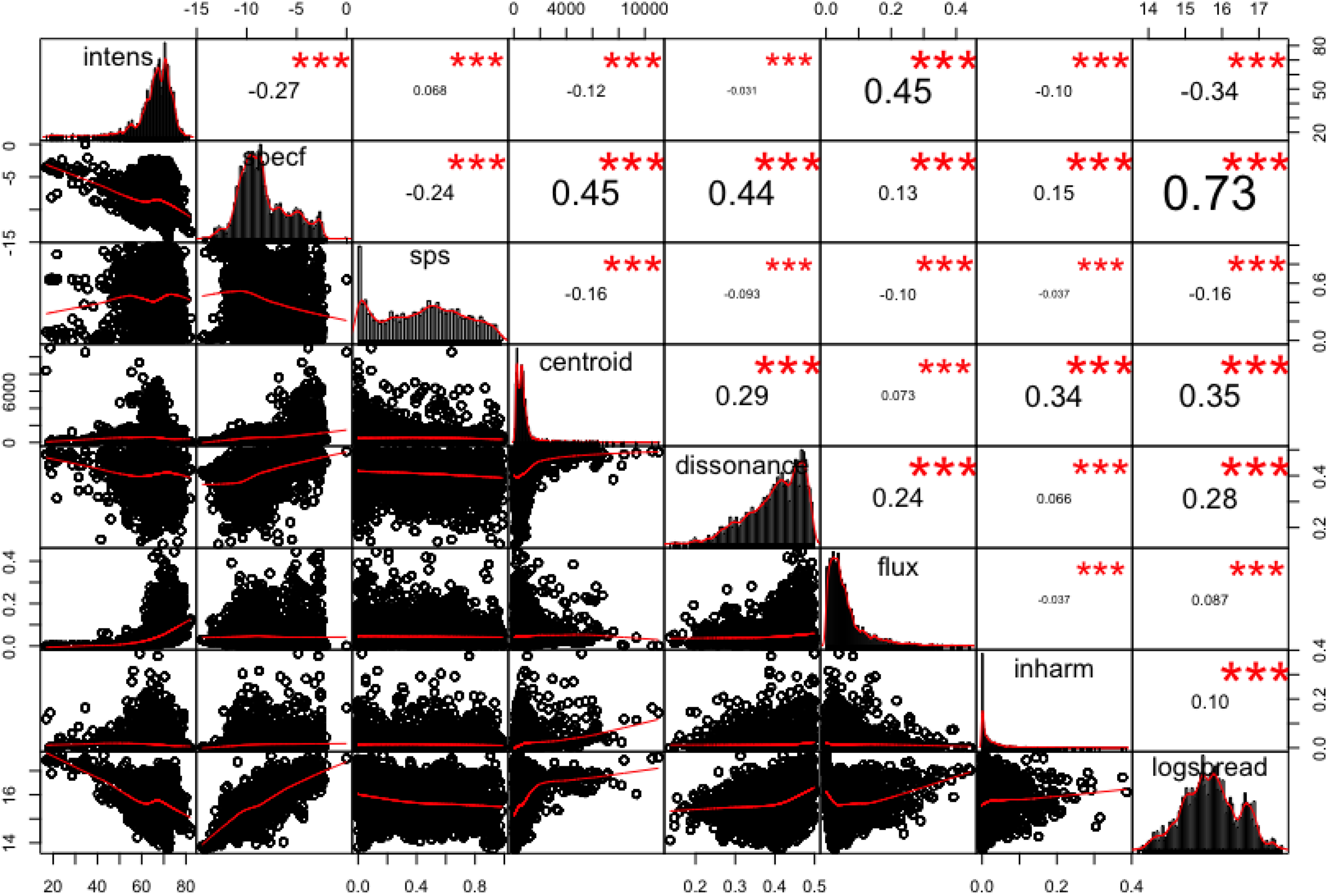
Acoustic features of Dataset 2 and their correlations. The diagonal shows the distributions of feature values for the eight parameters studied. The x-axis scale for each parameter can be seen alternately in the bottom and top line of the figure; the y-axis is shown alternately on the left and right. The other graphs show the scatter plots and the fit for each pair of features (and the measured correlation and probability level for each plot is shown in the square placed symmetrically on the opposite side of the diagonal). The features are in order along the diagonal: acoustic intensity; spectral flatness; SPS; spectral centroid; roughness (labelled dissonance); spectral flux; inharmonicity; and log (spectral spread). *** indicates significance at p < .001 (for all correlations).
Given the high noise content, signal–noise separation was used to remove the noise floor prior to smoothing and calculating cosine similarity. The method used to achieve this signal–noise separation is detailed in (Sethares, Milne, Tiedje, Prechtl, & Plamondon, 2009). For each component of the spectrum, the median magnitude is calculated across a centred window of 40 bins. If the magnitude of that component is less than noiseFactor times the window’s median, it is considered noise and removed. The parameter noiseFactor, therefore, controls the threshold between signal and noise. After preliminary investigation of the spectral patterns obtained from several of our target pieces, including comparison with conventional Fast Fourier Transform spectra, this was set throughout the analyses at 3. A consequence of this is also that some audio frames in our analysis, where there are no discrete spectral peaks (rather all sound is within the energy range of the noise floor) do not contain any usable frequency values: that is, at least one of the spectral pitch vectors is all zeros and so cosine distance is mathematically undefined (it is 0/0). Thus, in order then to measure cosine similarity between successive frames, a minimal amount of random statistical noise (a small multiple of MATLAB’s “eps,” the floating-point relative accuracy parameter) is added to each, to ensure that vectors always contain at least very small values. Such addition of statistical noise is commonly used for similar purposes, for example, in cepstral analyses. Cosine similarity measures, such as SPS, are favorable from the point of view of emphasizing spectral pattern similarity since, like correlation, they are unaffected by alterations in overall acoustic intensity levels (unlike spectral flux, which uses a Euclidean metric that is sensitive to overall magnitude).
Acoustic intensity and spectral flatness time series (2 Hz) were obtained in the earlier work using Praat (version 5.0, Boersma 2001).
In brief, intensity corresponds to unweighted sound pressure level (SPL) in dB. Spectral flatness is measured as Wiener Entropy, expressed on a log scale from 0 to minus infinity (the latter corresponds to an infinitely thin spectral peak, the former to white noise). For the modeling of the second, nine-piece dataset, there was sufficient data to allow the assessment of additional potentially salient acoustic parameters. Based on prior work on both isolated sounds and continuous timbral music (Olsen et al., 2016; Peeters, Giordano, Susini, Misdariis, & McAdams, 2011; Siedenburg, Fujinaga, & McAdams, 2016) we chose five additional features from the Essentia toolbox (Bogdanov et al., 2013): centroid (which measures the weighted frequency mean of the spectrum); flux (which measures jointly progressive changes in intensity and spectrum); inharmonicity (as above); “dissonance” (as it is named by Essentia, but perhaps better termed roughness, the term we will use below); and spread (a measure of how concentrated the spectral energy is with respect to frequency range).
Autoregressive Time Series Analysis (TSA) and Cross-Sectional Time Series Analysis (CSTSA)
Discrete time series of many processes, for example in physics, movement, physiology, and psychology, including perceptions of musical change and affect, are autocorrelated. This means that to some degree the value of the next event in the time series is predictable from some set of the preceding values. In the case of perceptions of musical change, lags (that is, previous events) of up to about 10 sampled at 2 Hz (i.e., 5 seconds) may be predictive. This means that conventional correlational and regression approaches are not applicable to modeling such time series (reviewed in Dean & Dunsmuir, 2016). Extensive specialized techniques of TSA have thus been developed to deal with such data. TSA models represent the autoregression of the dependent variable. They also consider the impact of lags of other potential predictors, which may be exogenous (i.e., for present purposes, uninfluenced by the dependent variable), such as the acoustic temporal features of a musical piece whose perception is studied, or endogenous (i.e., potentially mutually influential or influenced by the dependent variable). In the present study we have no endogenous variables to consider, and we deal with univariate time series analysis: a tutorial on these methods in relation to musical perceptions is available (Dean & Bailes, 2010). We also mention a type of multivariate TSA, called Vector Autoregression, which allows the assessment of interactions between endogenous variables. Especially in univariate TSA, it is important to ensure that the studied time series are statistically stationary, which means that the mean, variance, and the autocorrelations of the series variable are constant across the time series. When raw time series are not stationary, stationarity is commonly achieved by differencing the series: that is, constructing a series whose values are the differences between successive pairs of values from the original series; this was required here in some cases (as detailed later). Such stationary differenced series normally have zero means.
CSTSA is a mixed-effects version of time series analysis, which allows the simultaneous analysis of a panel of time series gathered from different individuals in response to a given stimulus (the data are sometimes termed “panel” or “longitudinal” data). Each individual series is preserved in the data and model, and possible random effects on groups, participants, or items can be considered. In our case observed random effects described the different propensities of individuals to autoregress their change responses. There were no significant random effects of pieces’ or participants’ propensities to induce perceived change (such as random intercepts: this is not expected with zero mean differenced series in any case), as distinct from the general power of acoustic intensity or SPS kinetics to influence these perceptions as fixed effects. As with mixed-effects analysis in general, the approach strengthens the statistical power of the assessment of the fixed effects—the response propensities shared across individuals—which is here the main issue of concern. Detailed discussions of CSTSA in analysis of continuous responses to musical affect are available (Dean et al., 2014a, 2014b).
For Dataset 1, we modeled the grand average response of the group of non-musician listeners using autoregression together with up to 5 lags of the acoustic predictors under consideration to create AR (autoregressive) and ARX (autoregressive with external predictors) models. Five lags were chosen, on the basis that all but one response series was of order 5 or less in its autoregression (as judged by the automatic ARIMA [auto-regressive integrated moving average] auto.arima function in the R “forecast” package) , and the choice was validated by the fact that no resultant model required an acoustic predictor lag beyond four. Models of perceived change in this dataset have been presented previously (Bailes & Dean, 2012; Dean & Bailes, 2010) and the extension here was to test the possible role of SPS.
The more powerful and general analyses were done with the larger Dataset 2, involving nine diverse musical extracts. Models of perceived change in this dataset have not been published previously; rather, the dataset has been used to investigate perceptions of larger scale musical structure and to model influences of acoustic and other factors on perceived affect (Dean & Bailes, 2016). In our CSTSA using every individual participant response series within the model, up to 5 lags were again permitted in each case, both to match the earlier analyses and on the basis of separately estimated order criteria using Vector Autoregression in the “vars” package in R. This also constrained the number of potential predictors under assessment (circa 45 fixed effects including the autoregressive lags) to an appropriate range (substantially smaller than the number of events) even given that the shortest excerpt under study had only 160 time series events, though many repeated responses. We used the R lme4 package for these analyses.
In each case, we start with a model containing all the candidate variables for the particular stage of analysis (as defined below) and proceed to model selection based on balancing precision of fit with parsimony. Thus, individually insignificant predictors are removed unless their removal substantially worsens the root-mean-square error (RMSE) between prediction and data, and within those constraints we seek a minimization of the Bayesian Information Criterion (BIC), which is also a primary defense against overfitting since it penalizes strongly for the addition of predictors. In the case of the CSTSA, the inclusion of design-driven random effects (i.e., random effects on intercept for participant and piece) brings a complexity to the interpretation of degrees of freedom in the analysis, and hence to the BIC, and so after removal of insignificant predictors it is used only as a guide (together with the RMSE) prior to final selection by means of likelihood ratio tests (where two nested models can be compared to determine whether one is probabilistically better than the other, and without a positive result the simpler is chosen).
In all cases, residuals are assessed for any significant remaining autocorrelation (which might indicate an inadequately specified model). This is done by means of partial autocorrelation functions (PACF), which assess the direct influence of lag n on the present event while quantitatively discounting for the fact that if lag n influences lag n − 1 (1st order autocorrelation), then to some degree lag n inevitably influences lags n − 2…n − 3, etc. indirectly. Models are accepted providing there are no significant low-order correlations in the PACFs and few others of considerable magnitude: with a p < .05 criterion for the significance of PACFs, one expects by chance 1 in 20 PACF lags that breach the significance limit. In some cases, the PACF quality criterion required the addition of AR components in order to achieve a satisfactory quality of residuals. Such selection approaches have been discussed in detail in our earlier work (Dean & Bailes, 2010; Dean et al., 2014a).
Results
Roles of SPS in Models of Perception of Change in Dataset 1
Here we consider whether SPS can contribute to models of perception of change in four pieces of unfamiliar music, based on our earlier models of these data (as shown in Tables 1 and 2, the pieces comprise excerpts of piano music by Webern, and of electroacoustic music by Xenakis, Wishart, and Dean). We ask sequentially: Does SPS alone enhance the optimal purely autoregressive time series models (Type 1 models) of continuous perception of change? Does SPS contribute to such a model to which the previously studied parameters spectral flatness and acoustic intensity are also added as potential predictors (Type 2 models)?
The time series of the continuous perception of musical change were not stationary and required first differencing to attain this. Thus, the models concern the first differenced series; as noted above, SPS already represents the difference between successive pairs of time samples, and so does not require differencing.
Tables 3 to 6 shows the key results of these models. For the Webern piano music example, the perceived change time series was close to level stationarity, but for comparative purposes here we chose to model its first difference, as with the other time series. We labeled the first difference of a series such as “perceived change” as “dchange.” A positive value of dchange means that perceived change has increased relative to perceived change from the previous lag; a negative value of dchange means that perceived change has decreased relative to the previous value of perceived change.
Webern.a

Note. AR = autoregression; sigma2 = measure of the mean error between predictions and data; SPS = spectral pitch similarity; BIC = Bayesian Information Criterion; dvariable = first-differenced form of a variable, lndvariable indicates its nth lag; ar = autoregressive lag; intens = acoustic intensity; specf = spectral flatness. For all three models:
Significance codes: 0 ‘***’ .001 ‘**’ .01 ‘*’ .05 ‘.’ .1
aThree different types of models were assessed: (a) purely autoregressive, (b) one which considers the possible impact of SPS alone, and (c) one which considers SPS acoustic intensity, and spectral flatness. In each case, lags up to 5 are considered. Log likelihood values characterize the model in relation to the data (higher values are better), while the BIC values summarize the efficiency of the model (lower values are better). Log likelihood and BIC values can only be compared across models of an individual series, whereas sigma2 values should be considered in relation to the mean and SD of the series being modeled, but then have broader comparability.
Xenakis.a

Note. AR = autoregression; sigma2 = measure of the mean error between predictions and data; SPS = spectral pitch similarity; BIC = Bayesian Information Criterion; dvariable = first-differenced form of a variable, lndvariable indicates its nth lag; ar = autoregressive lag; intens = acoustic intensity; specf = spectral flatness. For all three models:
Significance codes: 0 ‘***’ .001 ‘**’ .01 ‘*’ .05 ‘.’ .1
aThree different types of models were assessed: (a) purely autoregressive, (b) one which considers the possible impact of SPS alone, and (c) one which considers SPS acoustic intensity, and spectral flatness. In each case, lags up to 5 are considered. Log likelihood values characterize the model in relation to the data (higher values are better), while the BIC values summarize the efficiency of the model (lower values are better). Log likelihood and BIC values can only be compared across models of an individual series, whereas sigma2 values should be considered in relation to the mean and SD of the series being modeled, but then have broader comparability.
Wishart.a
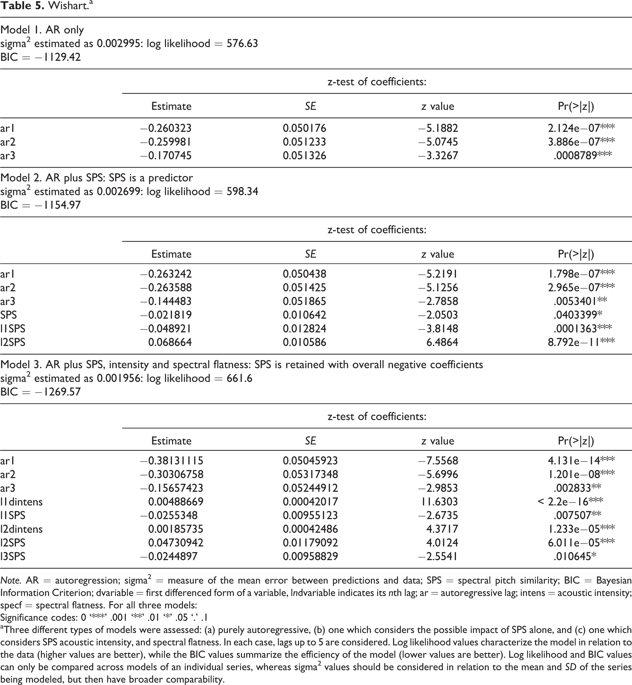
Note. AR = autoregression; sigma2 = measure of the mean error between predictions and data; SPS = spectral pitch similarity; BIC = Bayesian Information Criterion; dvariable = first differenced form of a variable, lndvariable indicates its nth lag; ar = autoregressive lag; intens = acoustic intensity; specf = spectral flatness. For all three models:
Significance codes: 0 ‘***’ .001 ‘**’ .01 ‘*’ .05 ‘.’ .1
aThree different types of models were assessed: (a) purely autoregressive, (b) one which considers the possible impact of SPS alone, and (c) one which considers SPS acoustic intensity, and spectral flatness. In each case, lags up to 5 are considered. Log likelihood values characterize the model in relation to the data (higher values are better), while the BIC values summarize the efficiency of the model (lower values are better). Log likelihood and BIC values can only be compared across models of an individual series, whereas sigma2 values should be considered in relation to the mean and SD of the series being modeled, but then have broader comparability.
Dean (no new model 2 was developed as SPS alone was not effective).a
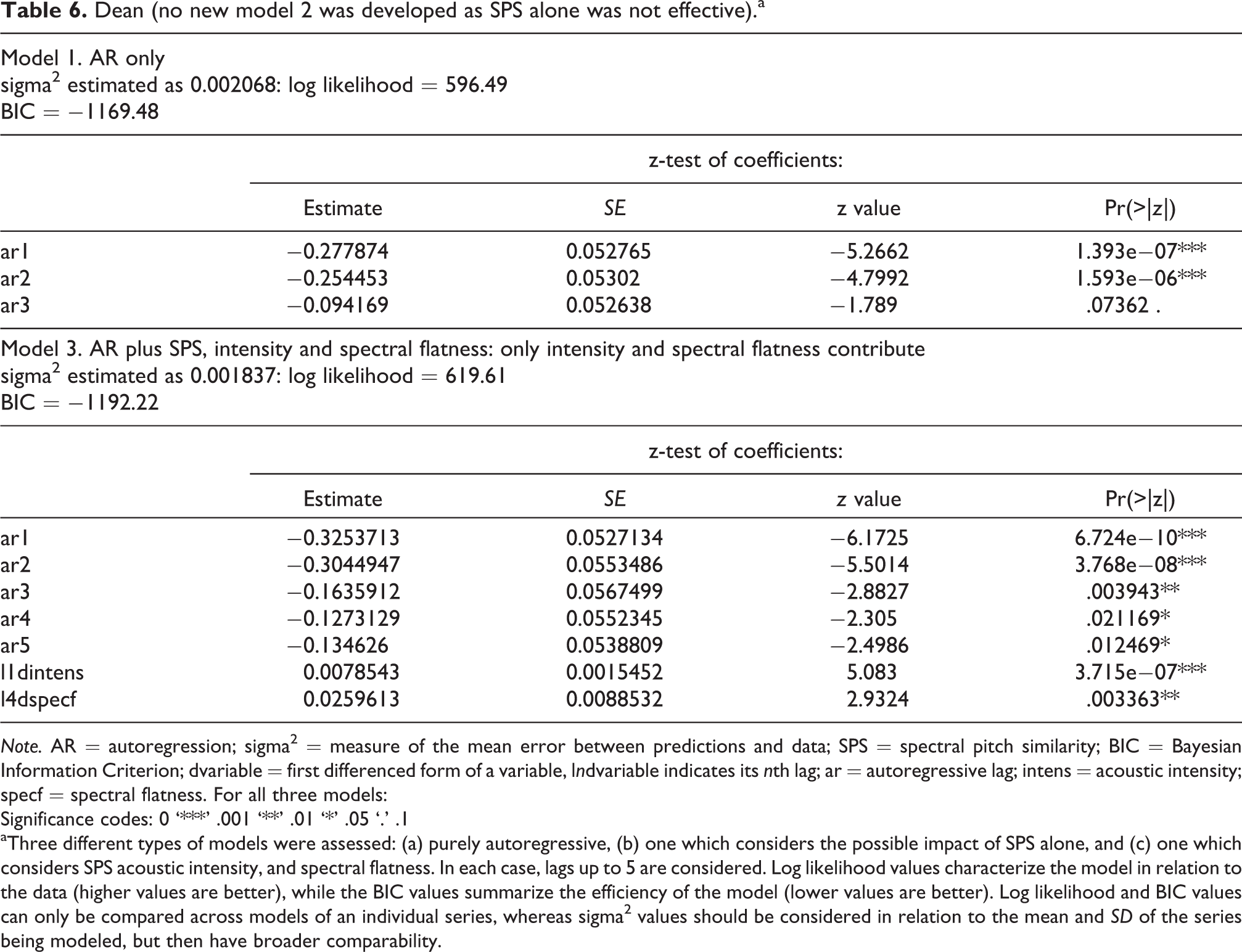
Note. AR = autoregression; sigma2 = measure of the mean error between predictions and data; SPS = spectral pitch similarity; BIC = Bayesian Information Criterion; dvariable = first differenced form of a variable, lndvariable indicates its nth lag; ar = autoregressive lag; intens = acoustic intensity; specf = spectral flatness. For all three models:
Significance codes: 0 ‘***’ .001 ‘**’ .01 ‘*’ .05 ‘.’ .1
aThree different types of models were assessed: (a) purely autoregressive, (b) one which considers the possible impact of SPS alone, and (c) one which considers SPS acoustic intensity, and spectral flatness. In each case, lags up to 5 are considered. Log likelihood values characterize the model in relation to the data (higher values are better), while the BIC values summarize the efficiency of the model (lower values are better). Log likelihood and BIC values can only be compared across models of an individual series, whereas sigma2 values should be considered in relation to the mean and SD of the series being modeled, but then have broader comparability.
In each case, an AR-only and an ARX model are developed.
No new model was developed.
In essence, the results given in Tables 3 to 6 showed that for two of the three electroacoustic sound-based pieces, SPS contributed to the first type of model and for one of the second model type. For the note-based piece of Webern piano music, SPS was again useful in the first model type, but acoustic intensity and spectral flatness supervened in the second. It is important to understand that time series predictors (like the autoregression of the predicted variable) are commonly effective over several lags, and the exclusion of a lag (such as lag 4) within a set from 1–5 is merely indicative that the size of its impact is too slight to achieve individual statistical significance. What counts for the model is the cumulative mathematical model and the potentially parallel perceptual impacts. Generally, the coefficients on SPS were cumulatively negative, as would be expected for the dependence of perceived change on a parameter that measures similarity (see below for in-depth analysis of the sign and magnitude of the impact of SPS in relation to Dataset 2). For the note-based piece, the time-based frames do not necessarily coincide with note events, and for a parameter such as SPS, this almost certainly drastically underestimates its predictive impact. While these results revealed only modest influences of SPS, it is to be expected (and is commonly observed) that different spectral features are accentuated in different sonic environments and different compositional styles (e.g., spectralist composition vs. noise music). For example, the pieces Bohor (Xenakis) and soundAFFECTS (Dean) are clearly driven largely by noise and acoustic intensity. Thus these initial results were sufficient to encourage us to perform a stronger and more general test of our hypothesis that SPS is a useful predictor of perception of musical change and, notably, that this is so even in sound-based music that does not emphasize the pitch and harmonic tones sounded on acoustic instruments in note-based music.
Roles of SPS in the Diverse Pieces of Dataset 2
In the second analysis, which was more general and wide ranging (given more extensive data), we considered whether SPS in the context of a range of other spectral parameters can contribute to new cross-sectional time series predictive models of perception of change in nine diverse pieces, both sound- and note-based, together with hybrid work. No previous modeling of continuous perception of change in these pieces has been undertaken, rather they have been studied in relation to continuous perception of affect (e.g., Dean & Bailes, 2016). The pieces ranged from Australian indigenous music to Miles Davis, electroacoustic music, and sound-text, as summarized in Tables 1 and 2.
Before commencing the CSTSA, we considered the possible correlation of the eight acoustic features being studied across the music excerpt Dataset 2. Note that, except for SPS, these were already chosen on the basis of prior studies of their relative independence in short sounds (Peeters et al., 2011) and their utility in studies of timbral phrase detection (Olsen et al., 2016). Figure 1 shows the distributions of the measures across 500 ms segments of the whole corpus (treating each segment as an independent sample from the whole set) and the Pearson correlations between them. For example, Figure 1 shows a correlation of .73 between spectral flatness and log(spectral spread), but no other correlations exceed .45. Interestingly, for SPS the strongest correlation with any other measure is only −.24 with spectral flatness. As expected from the nature of its construction (cosine similarity, see introduction) SPS does not show a correlation with acoustic intensity, whereas spectral flux has a much higher correlation (.45). SPS, showing limited correlations with other analyzed features, is thus a promising predictor to consider in models of perceived change. The more highly correlated variables did not coexist in the selected models, as might be expected.
A preliminary CSTSA model of perceived change, using the native (undifferenced) continuous perception series, suggested SPS was a predictor, but provided unsatisfactory residuals, retaining significant partial autocorrelations. Correspondingly only 27 of the 188 perceived change time series were stationary, thus it was necessary to model the differenced series (which stationarized the remaining series). The acoustic predictors were also differenced, accordingly (with the exception of flux and SPS, which are already measures that reflect the difference between adjacent frames of the time series). The data and predictors were then standardized, given the very different scales on which some of them are expressed (i.e., each was expressed in terms of a mean of zero and a standard deviation of 1). The optimized model of the standardized differenced series set is shown in Table 7.
Cross sectional time series analysis of Dataset 2. Linear mixed-model fit by restricted maximum likelihood. Model: dchange ∼0 + dintens + SPS + flux + dinharm + l1dchange + l1dintens + l1dspecf + l1flux + l1dspread + l2dchange + l2dintens + l2dspecf + l2flux + l2dspread + l3dchange + l3dintens + l3dspecf + l3dcentroid + l3dspread + l4dchange + l4dintens + l4dspecf + l4SPS + l4flux + l4dinharm + l4dspread + l5dchange + l5dintens + l5dspecf + l5flux + l5dspread + (l1dchange + l2dchange + l3dchange + l4dchange + l5dchange + 0 | pid).

Note. dvariable = first differenced form of a variable, lndvariable indicates its nth lag; change = perceived change; intens = acoustic intensity; SPS = spectral pitch similarity; flux = spectral flux; inharm = inharmonicity; specf = spectral flatness; spread = spectral spread; centroid = spectral centroid; pid = participant ID.
The model quality was acceptable, in that residuals from most individual series showed no partial autocorrelations in their PACF, the few positive PACFs were all small, and most were at longer lags than those modeled. As mentioned, occasional positive PACF coefficients can be expected by chance. The residual SD was 0.864, and the correlation between the model predictions and the data was .51. The model obtained involved the same predictors as those selected in the preliminary model of the undifferenced and unstandardized data. Here the random effects were developed first by considering intercepts, which given the differencing were, as expected, found to be 0. Then we considered possible random effects on the strongest predictors, which were the autoregressive components, and all lags were found valuable to the model in relation to participants, but not in relation to items (that is, the different musical pieces).
SPS had overall a slight negative coefficient, as expected. A direct test was made of whether the removal of all the SPS components worsened the model; both the residual standard deviation and the likelihood ratio test showed that the full model was much better than that omitting SPS (p < .00001 that they were indistinguishable).
Figure 2 shows the modeled response of the system to a unit increase in SPS, flux, or intensity, where a unit increase is that of 1 SD of the predictor in question and the dchange response parameter is measured in the same terms. This is termed the “impulse response” and, in the case of CSTSA, describes fixed (population-wide) effects. The impulse response is computed by repeatedly applying the terms and coefficients of the models given a 1 SD increase in the specified predictor to predict the consequent changes at each successive lag. As often observed, putting aside autoregression, changes in acoustic intensity are the dominant predictor for perceived change: the sum of the 11 sequential impulse responses values, being closely related to the integral under the response curve, was 0.295. Increasing SPS had a small net negative effect (sum of response values = –0.003), as predicted. This indicates that the more spectral pitch cosine similarity decreases, the stronger the positive impact on perceptions of musical change. Again, consistent with predictions, increasing flux had a small positive effect (sum = +0.004).
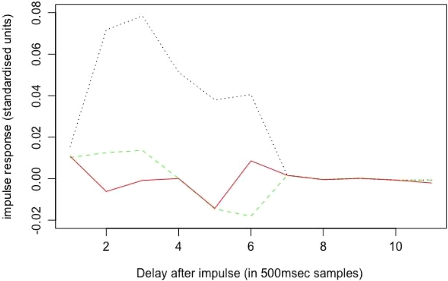
Impulse response functions for a 1 SD increase in first differenced intensity, flux and spectral pitch similarity change (SPS). Dotted, black line = dIntensity; dash, green = flux; solid, red = SPS; dvariable indicates the first differenced form of a variable. The response units are also SD of dchange. A positive value of dchange means that perceived change has increased relative to perceived change from the previous lag; a negative value of dchange means that perceived change has decreased relative to the previous value of perceived change.
The model and the results of Figure 2 are consistent with our hypothesis. Thus, as often observed, changes in intensity have large impacts on perceived change (the two rise together), while the influences of spectral parameters are much smaller. And as spectral flux increases, or SPS decreases (becomes more dissimilar), so perception of change increases. However, we should note that the spectral impulse response functions are slightly unrealistic, in that it is hard to alter SPS without influencing flux (although it is easier to alter flux without influencing SPS: e.g., by changing the intensity of either sound in the pair being compared). So, the impulsing variables in Figure 2 are not entirely orthogonal, and the interpretation of the figure must be taken cautiously. It is also important to recollect that Figure 2 describes the fixed effects component of the CSTSA model (that shared by the population of participants) but, given the random effects, the precise quantitative relationship between the predictors and the perceived change differs and thus impulse response functions (IRFs) vary quantitatively between individual participants; and the model specifies this through its random effects.
The model, in addition to roles for flux, intensity, and SPS, shows influences of centroid, flatness, inharmonicity, spread, but not of roughness (termed dissonance by the Essentia package). Crucially for our present core purpose, the data from the CSTSA continue to demonstrate a distinctive role for SPS in models of perceived change.
Discussion
SPS measures have been developed as an explanatory tool for the perception of tonal and microtonal note and chord stability or fit. In such situations, the indications are that many observations in the literature can be explained as well or better by models using SPS (or spectral pitch class similarity, which treats all pitches an octave apart as identical [Milne et al., 2015; Milne & Holland, 2016]), than they can by models based on familiarity (i.e., estimated exposure statistics when such data are available, which they cannot be for musical styles novel to a participant). Data on pitch-based melodies whose spectra were experimentally manipulated are consistent with independent impacts of SPS and inharmonicity on perceptions of fit (Milne et al., 2016). The present article extends these observations substantially, by applying SPS to pieces that include strong noise components or are, essentially, sound-based rather than note-based works (Landy, 2009). The utility of the feature as a predictor in models of perceived change indicates that its influence is likely to be general, rather than solely applicable to harmonic complex tones and their close relatives in note-based music. Inharmonicity again has a modest role to play (Table 7). Given that our previous work showed considerable commonalities in perceptions of musical change between different musical expertise groups, we would expect the results shown here for nonmusicians to be applicable also to musicians.
Furthermore, although spectral pitch (class) similarity between temporally adjacent harmonic chords is not designed to provide an unmediated explanation of musical structure, it still plays a weak but significant role in characterizing patterns of chord sequences commonly found in classical, pop, and jazz musical styles, particularly the first (Harrison & Pearce, 2018). We suspect that, to better reflect the impact of spectral pitch (class) similarity on the structure of musical harmony, it will be necessary to extend this work also to consider relationships between non-adjacent chords. For example it is suggested that common cadential forms—ii-V-I, IV-V-I, iv-V-i, etc.—are characterized by a specific configuration of all three pairwise spectral similarities between the three cadential chords (Milne, 2010). Thus, the relevance of SPS to a wide range of genres within both note- and sound-based music is indicated. Taken together with the evidence in the present article on SPS in both note- and sound-based music, we can suggest that a bottom-up contribution of SPS is likely to be widespread, both in familiar and unfamiliar music or music genres.
The values of the key Gaussian smoothing width parameter used to calculate SPS has been taken from prior work (as described above); the value of the noiseFactor parameter, which determines the noise/signal threshold across all the pieces, was obtained by simple assessments of the effectiveness with which the spectral pattern of individual sound chunks is represented. In contrast, in earlier studies, while the noise-floor parameter was not required, the Gaussian smoothing parameter was optimized for its strongest predictive capacity in relation to individual datasets. In future work, optimizing both parameters of SPS in relation to novel datasets may be appropriate.
It will also be interesting to assess whether SPS is not only effective as a predictor of perceived “change in the music,” which might be considered a very basic, untrained capacity, but also in perception of affect (where appraisal, exposure, and expertise may have a little more impact, even though qualitative features generally remain the same between expert and inexpert listeners). For example, in pitch-based contexts, spectral pitch (class) similarity is an effective predictor of musical “fit” (Milne et al., 2015, 2016; Milne & Holland, 2016), which is a more abstract and musically informed appraisal than is “perceived change.” It seems natural to see if this predictive capacity extends to sound-based contexts, and to other affective appraisals such as valence and arousal. More generally, it is apparent that SPS may be a useful acoustic parameter in future studies of a wide range of music in music information retrieval (MIR) and music perception. The present correlative study will need to be extended by future work in which SPS is systematically transformed in some stimuli for causal analysis of its perceptual impact.
Conclusion
SPS, measured on denoised inharmonic and noise-bearing music, is a significant predictor of listeners’ perceptions of musical change therein. It is distinct from other major conventional spectral parameters in that it cooperates with them in the selected models of change perception. Thus, SPS has relevance to perceptions of musical change and of timbral relationships in a wide range of music, not just for instrumental music using complex harmonic tones.
Footnotes
Authors’ contributions
Experiment design, FB and RTD; modelling, RTD and AJM; writing, RTD, AJM, and FB.
Declaration of conflicting interests
The author(s) declared no potential conflicts of interest with respect to the research, authorship, and/or publication of this article.
Funding
The author(s) received no financial support for the research, authorship, and/or publication of this article.
Peer Review
Rie Matsunaga, Kanagawa University, Department of Human Sciences.
Kyung Myun Lee, Korea Advanced Institute of Science and Technology, School of Humanities and Social Sciences.