Quantitative analysis of temporal structure in Cuban guaguancó drumming

Abstract

We examine the temporal properties of cyclical drumming patterns in an expert performance of Afro-Cuban rumba recorded in Santiago de Cuba. Quantitative analysis of over 9,000 percussion onsets collected from custom sensors placed on various instruments reveals different types and degrees of rhythmic variation across repetitions of each of five characteristic guaguancó patterns (clave, cascara, quinto, segundo, and tumba). We assess each instrument’s variability using principal component analysis and multidimensional scaling, complementing our quantitative exploration with insights from music theory. Through these methods, we uncover details of timing that are insufficiently conveyed with standard music notation in order to shed light on the role of improvised variation in solo and accompaniment ensemble roles.

Introduction

With deep historical roots and encompassing a wide spectrum of styles, the Afro-Cuban musical repertoire holds in store incalculable rhythmic riches. An important contributing factor to this is the spontaneous creativity of performers who phrase the music in real time with a unique rhythmic “feel”. Even when reading from a notated score (not the norm in many Cuban musical communities), and especially if performing without one, expert Afro-Cuban musicians shape rhythm in intricate ways that lend themselves well to quantitative description and analysis. In the present study, we use a combination of music theory and quantitative methods to examine the temporal properties of individual interlocking layers in an ensemble groove.

Particularly intriguing – for curious outsiders like ourselves – is the interplay between repetition and variation. If a performer has the freedom to transform a rhythm through variations, what forms do the variations take? Investigating the dialectical relationship between theme (or repetition) and variation (or change) has been a focus of the ethnomusicology of many non-Western traditions. This is partly due to the fact that standard Western notation is not calibrated to accurately represent the kinds of dynamic, gestural, temporal, and timbral variations that are common and important in many non-Western musics. Quantized to fit within the rough-grained resolution of Western notation, and trapped between repeat signs, the rich variations of many African-diasporic, Southeast Asian, and Native American musics (for instance) dissolve into thin air. Many scholars – especially Diaz (2017), Gerischer (2006), McGraw (2008), Monson (1999), and Tenzer (2006) – have been concerned with recognizing, representing and analyzing these overlooked forms of variation. The present article is a contribution to this discourse.

This ethnomusicological discourse has often sought to nuance earlier, polarized descriptions of theme and variation as found, for instance, in Kramer’s (1988) association of repetition with stasis and variation with movement, Adorno’s (1990) denigration of repetition as a loss of critical individuality, Schuller’s (1989) conflation of repetition and boredom, and Rahn’s (1993) association of repetition with slavery. Iconic African-American authors have proposed alternate paradigms, such as Baraka’s (1963) concept of the “changing same” and Gates’s (1988) description of “repeating with a difference”. Within the ethnomusicological context, terms such as “sectional periodicity” (Tenzer, 2006, p. 26) describe a similar logic of ostinato-with-variations. Because theorists sometimes conflate “theme” with “restraint” and “variation” with “freedom”, the musical analysis of repetition and change within African-diasporic musics is a highly charged discourse within the context of historical oppression.

Another intriguing aspect of this repertoire is the way in which a given rhythmic sequence might differ from its representation in standard Western notation, be it a score that the player follows or a transcribed approximation that his or her playing instigates. In his pioneering work on Afro-Cuban rhythm, Alén (1995) laments the limits of music transcription to convey the temporal nuances of Cuban tumba francesa performances he and his colleagues had recorded in the field during the 1970s. Noting the lack of “a scientific musical notation system that will allow a more precise graphic representation of the music” (1995, p. 56), Alén’s analyses of instrument timing rely on duration measurements to quantify how repeating patterns differ from isochronous metric divisions. Bilmes (1993) also provides quantitative evidence of non-isochrony in Afro-Cuban drumming. Using onset detection and timing analysis algorithms to examine performances by Los Muñequitos de Matanzas, Bilmes argues that in order to adequately represent rhythmically “expressive” music, it is necessary to “leave the symbolic world” – by which he means the discreteness of metric structure – “and enter the continuous one” (1993, p. 19). More recently, Stover (2009) has illustrated how Afro-Cuban rhythm can be understood as operating in a fluid metric environment where the beat is “a scalable duration rather than a single instant in time” (p. 163). He further observes that such a framework is compatible with a blended conception of meter in which triple and quadruple grids are simultaneously active. Musicians enact this superposition not only across ensemble parts (with one player using triple division and another player using quadruple) but also within their own rhythmic phrasing. To indicate these nuances, Stover enhances his transcriptions with left- and right-pointing arrows above those notes that fall before or after their nominal metric position. In what follows, we offer detailed analyses of performed patterns to shed additional light on how complex Afro-Cuban rhythms can surpass the limits of music notation.

In this article we ask: what degrees of freedom are displayed by each of the interlocking rhythms in Cuban guaguancó? What are the rhythmic resources from which this freedom emerges, and what notational challenges emerge as a result? We address these questions as they arise in a specific recorded performance by an Afro-Cuban percussion ensemble. We show that the distinct cyclical patterns that characterize the interlocking layers undergo different modes of variation, and that these collective differences can be suitably examined by implementing a variety of quantitative approaches. Our primary approach employs principal component analysis (PCA), a technique that involves the transformation of a large set of variables into a smaller set of linearly uncorrelated variables described as principal components. This method allows us to visualize certain properties within datasets as well as to pinpoint prominent variations underlying the data. ¹ Interwoven with musical analysis, our quantitative exploration is a novel contribution to the understanding of musical rhythm in an ostinato-based improvisatory setting.

The dataset

In 2013 Andrew McGraw recorded a series of Afro-Cuban drumming performances using a custom sensor-based system designed to capture natural performances of percussion-based repertoires in field conditions. Individual piezo sensors running into a 24-track JoeCoe field recorder were placed on each of the instruments and did not interfere with instrument tone or playing technique. This mechanism allows for the complete isolation of instrumental onsets while preserving dynamic and pitch information, facilitating onset identification and timbre analysis (see McGraw, 2013; McGraw and Kohnen, 2016). The corpus includes recordings of Afro-Cuban rumba, tumba francesa, and bata repertoires by an expert ensemble led by Maestro Blas.

While most discussions of Afro-Cuban music have focused on styles from Havana and Matanzas, ² our dataset is drawn from a performance by a comparatively underrepresented community of musicians in Santiago de Cuba, located in the east of the island (Figure 1). In conversation, Blas described his ensemble’s performances as embodying a specifically “oriente” (Eastern) style of Afro-Cuban rumba. While Blas and his musicians also described their playing as distinctly “Santiago de Cuba style”, it appears strongly linked to the Havana style. This makes sense, given the strong demographic movements between Havana and Santiago de Cuba. Stylistic differences between rumba groups often emerge when local rhythms are incorporated into the Havana style, as when Afro Cuba de Matanzas developed the Bata Rumba, or when Folkloyuma of Santiago de Cuba developed the Rumba Conga (Peter Loman, personal communication). Santiago de Cuba is more commonly associated with the history of son (a progenitor of salsa) rather than with rumba. Nevertheless, our study suggests that more research needs to be done to ascertain the status of emerging styles specific to Santiago de Cuba. It might be the case that the defining features of these variations occur at the subtle level of timing described in this article.

Figure 1.

Map of Cuba, with Santiago de Cuba indicated.

In this article we focus on one of the three rumba recordings: the up-tempo guaguancó, a groove that typically accompanies a couple’s sensual dance (Daniel, 1995). The recording features five performers playing the set of instruments shown in Figure 2: three idiophones – the clave percussion sticks, a cowbell, and cascara temple block – and three conga drums of varying sizes and pitch ranges – the high quinto that performs complex improvisatory patterns, the medium-pitched segundo that keeps to a relatively fixed accompaniment pattern, and the lowest tumba (or tumbadora) that, in combination with a large cajón wooden box, also performs accompanying patterns with frequent rhythmic variation. ³ Because they were performed by a single player, the temple block and cowbell were mixed into a single track and treated as a single instrument (cascara), as were the tumba and cajón (tumba). This resulted in a total of five audio tracks, one for each of the five players (clave, cascara, quinto, segundo, and tumba) and containing only onsets produced by that player. Interested readers are welcome to contact the authors for more information about the recordings.

Figure 2.

Recording Maestro Blas and his group, with sensors affixed to instruments. From left to right: (1) Maestro Blas – temple block (cascara) and bell, (2) José Antonio Centray Casamayor – quinto, (3) Daniel Poyoux Vargas – segundo, (4) Nelson Silveira Despaigne – tumba and cajón, (5) Lázaro Dumoi Larrea – clave. Photo by Andrew McGraw.

A preliminary list of onset times for each player was prepared using Sonic Visualizer’s Aubio Onset Detector plug-in. The lists were then corrected manually – shifting, deleting, and adding markers as needed – to produce five time series accurate to within ±1 millisecond. Total onset counts for each player are as follows: clave (931), cascara (1,924), quinto (2,125), segundo (2,030), tumba (2,000). ⁴ Taking the first differences in the sequence of note onsets t ₁, t ₂,…yielded a sequence of note durations – also called interonset intervals (IOIs) – for each player. The performance covers 186 four-beat measures and lasts 5 minutes, 12 seconds; all five musicians play continuously. The performance begins with a tempo of 138 beats per minute (bpm), then increases quasi-linearly to 145 bpm roughly halfway, after which it holds fairly steady before decelerating slightly to about 143 bpm over the last 10 measures. ⁵

Preliminary analyses

Each of the five instruments features an identifiable repeating pattern of equivalent cycle length (one measure). ⁶ Their transcriptions appear in Figure 3. (Note that there are two cascara versions: one with 10 notes and another with 11.) The patterns exhibit different degrees of temporal variation across cycles, ranging from negligible change to overt continuous transformation. To obtain a preliminary overview of pattern regularity, we computed the power spectral density – which measures the amount of repetition at different time spans – for each of the five IOI sequences. ⁷ Because our input consists of a time series comprising note onsets indexed by note number rather than an audio signal consisting of sound pressure levels indexed by time, frequency in this case has units of cycles per note. For example, a repeating four-note pattern has a frequency of .25 (the reciprocal of four) because each note recurs every one fourth of a cycle. (One cycle is exactly one note position, so that one time per four cycles is the same as one note out of every four.) The power spectral density provides a useful quantitative summary of variability because patterns that repeat tend to concentrate their energy at the frequency of repetition, and the plot of such a pattern will have a sharp peak at that frequency. Conversely, less repetitive patterns such as those characteristic of improvisation tend to have power spectral density functions without clear peaks.

Figure 3.

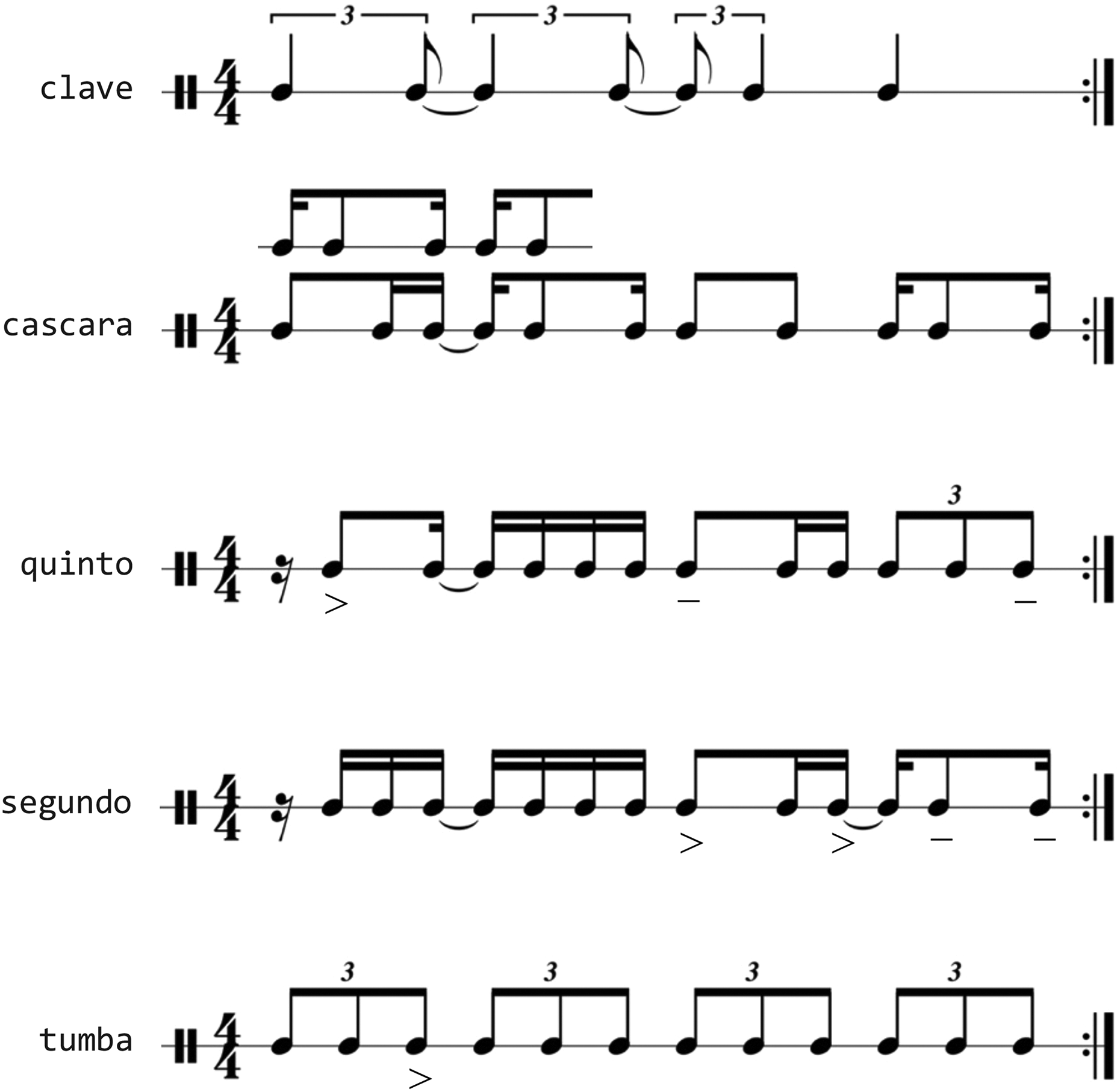
Transcriptions of individual rhythmic patterns. On the quinto and segundo, the articulation symbols > and – denote (respectively) an accented open tone and a slightly accented slap tone; pitch content is not displayed. The tumba pattern is played primarily on the cajón; the symbol > denotes an accented note.

Power spectral density plots of the five IOI sequences appear in Figure 4. The x axis is in units of frequency, or cycles per note, where a note is an IOI and a cycle is a sequence of IOIs that repeat (or repeat nearly so). The plot’s origin (left side of the x axis) represents a constant sequence of notes of identical duration; this is zero frequency since the undifferentiated string can be said to have no period at all (it repeats trivially). The maximum frequency is 0.5, which corresponds to a two-note pattern that repeats with no variance whatsoever. ⁸ The y axis (energy) represents how much of the signal’s variance can be described by an IOI sequence at any given frequency. If there is a large peak at some frequency, it is usually a good indication that the sequence of IOIs has at least a component that is periodic with that frequency.

Figure 4.

Power spectral density plots for the ensemble’s five instruments. The more repetitive instruments have clearer peaks (indicated with arrows).

The clave’s strong peak at 0.2 cycles per note indicates that the clave follows a strict five-note pattern with practically no deviations. There is also a strong secondary peak at 0.4. This is not only a harmonic (a multiple of 0.2, given the clave’s stable recurrence), but also evidence of the 2.5 notes-per-measure pattern that is embedded within the clave (short-long followed by short-short-long). ⁹ The cascara’s peak at 0.09 (equivalent to 11 notes/cycle) is broad enough to also cover 0.1 (10 notes/cycle). As we saw in Figure 3, the cascara has a 10-note and an 11-note version; these highly similar versions are essentially indistinguishable from the spectrum. Weak harmonics are also visible at 0.18 and 0.36, as well as an additional peak at 0.31. The latter stems from the embedded long-short-long (eighth-sixteenth-eighth) pattern that occurs three consecutive times starting on the downbeat of the 10-note version, and which takes up 5/16ths (0.31) of the measure. The quinto’s graph is mostly flat because of extensive variation, although a broad, low peak around 0.09 (11 notes/cycle) is just visible. The segundo’s peak at that same location is vastly more prominent, and is echoed by strong harmonics. Finally, the tumba’s flat power spectrum reflects its high incidence of rhythmic variation.

Another way to represent the contrasting degrees of regularity observed above is to compute a novelty function for each instrument, as shown in Figure 5. The function is calculated from an array whose rows represent measures and columns represent IOIs. ¹⁰ From this array, one can form a self-similarity matrix M_ij , in which each entry is the L ² (Euclidean) distance between measures i and j. Thus, if each measure is expressed as a vector of IOI values, calculating the Euclidean distance between two vectors gives a measure of how similar – or close together in Euclidean space – the measures’ rhythms are. Following the construction in Müller (2015), we constructed each novelty function by convolving M_ij with a checkerboard sign pattern to identify groups that differ from their neighbors. The novelty function is the result of this convolution along the diagonal after a low-pass filter (10 windows). ¹¹ The graph’s average novelty values are much lower for the clave and segundo than for the tumba and quinto, while the cascara – which switches between two fairly structured patterns – is intermediate.

Figure 5.

Novelty functions and mean novelty values (in parentheses) for each instrument across the entire performance. Lower values denote higher degrees of pattern regularity.

Individual patterns

In the following sections, we analyze each of the instruments in order of increasing novelty. To assess the nature of each instrument’s variance, we will work with two versions of the same data: sliding window array and measure window array. Figure 6 illustrates their design as applied to the clave’s five-note pattern. In both cases, an instrument’s sequence of onsets is parsed into windows of adjacent IOIs. We organize these windows in tabular form, so that each window corresponds to a row and each column corresponds to a position within the window. The main structural difference between the two arrays is that in the sliding window every subsequent IOI starts a new row, whereas in the measure window only the first IOI of each measure starts a new row. Therefore, while a given note appears multiple times in a sliding window array, it appears at most once in a measure window array. In addition, in order to eliminate any effects of tempo on variability, we linearly rescaled measure window arrays to “relative time” by converting IOIs to percentages of the measure that contains them. Using two types of array allows us to probe the data from different perspectives – sliding windows give a more rudimentary description of variability while measure windows (requiring human intervention to locate the start of each measure cycle) afford a sharper focus on pattern behavior. This distinction is trivial in the case of the clave but becomes especially meaningful with more “noise-like” patterns.

Figure 6.

Extracting a sample of measures (right) from the clave’s sliding window array (left). In both frames, the color of a cell indicates the interonset interval in seconds. In the measure window array, columns correspond to intervals between notes; notes are sounded between columns.

Regardless of how the window array is formed, our subsequent analysis treats each row as a vector whose components are given by the row’s columns. Each vector is a point in high-dimensional space, forming a point cloud that carries an abstracted representation of the structure of the music. Empirically, most of these point clouds are confined to a lower dimensional subspace whose dimensions describe the degrees of freedom that the performer is exploiting in the recording. Different performers on different instruments exhibit vastly different amounts of variability, and in musically different ways.

Principal component analysis (PCA) provides a quick visualization of the point cloud. We introduce each forthcoming section with a PCA plot of the instrument’s sliding window array. These are scatter plots showing each sliding window as a point. The axes are chosen to maximize the variance of the data while minimizing distortion to the relative distances between windows. More specifically, the horizontal axis is chosen so that the largest variance in the data lies along this axis, while the second largest variance lies along the vertical axis. The scatter plot therefore provides a good overview of the variability in the IOI sequence. We then switch to the instrument’s measure window array to display the principal eigenvector, which characterizes the changes that capture the majority of the variability across measures. In other words, the principal eigenvector shows the rhythmic adjustments that the performer typically makes. If most of the variability is captured by coordinated change of two notes – one arriving earlier while another arrives later, for instance – this is clearly illustrated by the principal eigenvector.

Clave

Figure 7 shows the PCA plot (left panel) for the clave’s first two principal components – the dimensions along which most of the variability occurs – and the eigenvalues (right panel) for the first 13 principal components. We see in the PCA plot that the clave’s five-note repeating pattern contains almost no variation, as is customary of timeline rhythms such as the clave (Peñalosa, 2012). Moving along one of the PC axes corresponds to changing a single degree of freedom in the pattern, such as changing the value of a single IOI or several IOIs simultaneously. In the graph, each of the clave’s five notes forms a (color-coded) cluster that is connected to exactly two adjacent clusters; over time each cluster is entered along one green edge and exits along the other to form a distinct star shape. ¹² The clusters are sufficiently well-separated that they can be identified algorithmically using “k means ++” (Arthur & Vassilvitskii, 2007); as we will see, this automatic identification fails for the tumba and quinto, which exhibit much greater variability in their temporal structure.

Figure 7.

Clave’s first two principal components (left) and first 13 eigenvalues (right) under a sliding window array.

Figure 8 shows the clave’s dominant eigenvector. The dominant eigenvector points along the dimension (of the high-dimensional point cloud) to which most of the variability is confined. Since eigenvectors in this article are composed of IOIs, the x axis contains one interval fewer than there are notes in the pattern. ¹³ The y axis expresses the amount of change in the length of the IOI for each note listed in terms of its position in the measure. The units in the y axis are relative and should not be ascribed absolute meaning in terms of typical note displacements. ¹⁴ The clave’s graph shows that the variation in that direction corresponds to decreasing the first and second IOIs while at the same time increasing the fourth IOI. This corresponds to simultaneously moving the second and fifth notes (the pattern’s two long notes) in opposite directions – if one happens earlier, then the other happens later.

Figure 8.

Components of the clave’s dominant eigenvector using a measure window array. There are four values for the five-onset pattern because each eigenvector corresponds to an interonset interval, of which there is always one less than there are onsets.

Musicians who study and perform Cuban music often distinguish between two versions of clave: one uses quadruple subdivision and the other uses triple. While the clave in this recording is essentially triple, its timing is consistent with a specific rhythmic routine that does not conform to the metronomic divisions of an isochronous metric framework. Figure 9 shows median durations – scaled as percentages of measure duration – for the five notes in the clave pattern across 186 cycles. Only the first and last notes tend toward deadpan values (the quarter-note triplet and quarter-note, respectively). The other three notes tend to be either shorter (notes 2 and 4) or longer (note 3). Viewed from the perspective of onset placement within an idealized 12-slot grid, these values translate into an early note 3 (because note 2 is short) and a late note 4 (because note 3 is long); these two forces more or less cancel each other out so that note 5 coincides almost exactly with the idealized location of the measure’s fourth beat.

Figure 9.

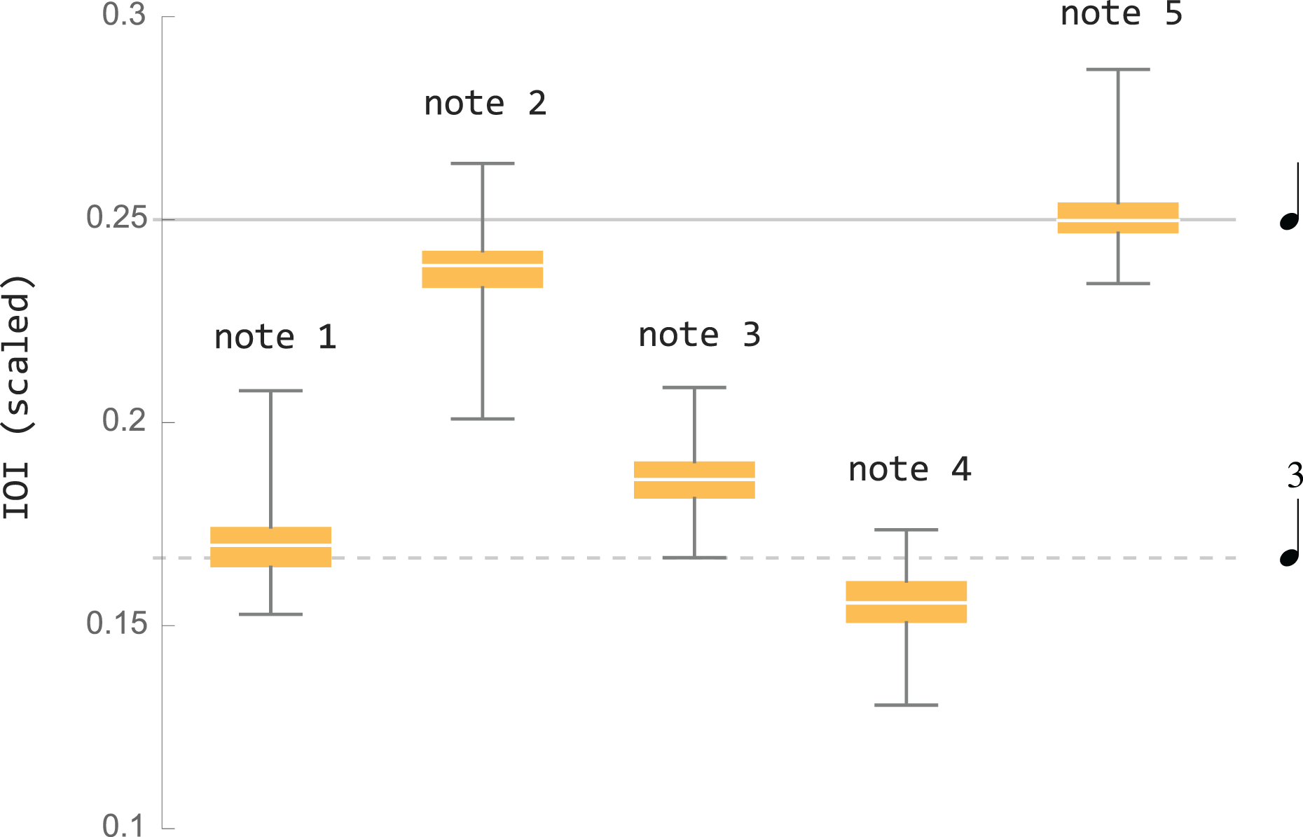
Clave’s median interonset intervals (IOIs), scaled as relative (percentage) durations of the measure cycle and showing distribution of values. The two horizontal lines give deadpan duration values for the quarter-note (0.25 of the measure) and quarter-note triplet (0.167 of the measure).

This temporal profile remains basically stable throughout. However, the increasing tempo does not affect all notes in the pattern uniformly; the timing structure of the clave varies – albeit marginally – with overall tempo. At the faster tempo, the interval between notes 1 and 2 does not shrink (as it does with the subsequent pairs), which results in note 1 being proportionally longer during the faster (later) section of the performance compared to the slower (earlier) one. This can be seen in Figure 10, which plots raw (orange, left axis) and scaled (blue, right axis) durations for notes 1 and 2 across the 186 measures. Note 1’s proportional value, but not its raw value, is lower at the beginning of the performance, when the tempo is slower. By contrast, both the raw and proportional values of the other notes (only note 2 is graphed) decrease with the rising tempo. ¹⁵ Even though this effect is probably too small to have perceptual significance, we point it out to highlight the notion that performative gesture – by which we mean physical movement as well as the resultant characteristic of the performance – is not independent of cycle speed.

Figure 10.

Clave interonset intervals (IOIs) for the first two notes of the five-note pattern. Orange and blue plots correspond to actual and scaled values, respectively. A 16-measure moving average window was used to smooth out the visualization.

Segundo

The PCA plot and eigenvalues for the segundo are shown in Figure 11. The PCA plot reveals a clear 11-note pattern over the course of the performance, with intermittent variants visible as outliers. (As with Figure 7 above, the axes are in units of relative position within the measure and do not represent units of time.) The eigenvector in Figure 12 shows that the third IOI is the main source of variance: when the fourth note comes earlier or later, it delays or advances the rest of the notes in the measure. ¹⁶

Figure 11.

Segundo’s first two principal components (left) and first 13 eigenvalues (right) under a sliding window array.

Figure 12.

Components of the segundo’s dominant eigenvector using a measure window array.

Just as the clave is closely aligned with a triple division of the beat, the segundo is primarily – if loosely – quadruple. The histogram in Figure 13 shows the segundo’s distribution of onsets within the four-beat measure cycle. ¹⁷ Since the segundo tends to play about 40 ms ahead of the clave (which sets the cycle downbeats for this graph), the histogram is shifted rightward by one fortieth of a measure to maximize alignment with a quadruple grid. But even thus shifted, the loose fit is evident; the local peaks do not line up neatly with the quadruple-division coordinates.

Figure 13.

Placement of segundo onsets within the four-beat measure cycle. Vertical coordinates mark nearby quadruple subdivisions of the measure. Onset placement is calculated proportionally from the full duration of the measure in which it appears. Each beat spans approximately 425 ms (the tempo varies across the performance).

Two types of variation take place in the segundo, both of which introduce a triple-division twist to the otherwise ostensibly quadruple pattern. ¹⁸ The first type of variation involves an adjustment to the timing of the pattern’s basic template. The second type is a more salient departure from the basic pattern. We will examine both types in turn and address the inability of standard Western music notation to account for their rhythmic makeup.

The segundo pattern is generally taught and performed in the version shown in Figure 3 above. The first beat’s last note is a sixteenth-note tied to another sixteenth-note (amounting to one eighth-note), and the next beat’s first note – the pattern’s fourth onset – is a sixteenth-note as well. When the pattern is first heard in the second measure of this performance, it is a faithful reproduction of that version, one where note 3 is twice the duration of note 4. One measure later, the durational contrast between notes 3 and 4 is less stark; the two notes are now slightly more even. The equalization trend continues with subsequent repetitions so that 30 measures later note 3 is about 8% shorter than note 4 – a clearly audible makeover of the original sequence.

This new version is maintained throughout the remainder of the performance. Figure 14 shows the gradual transition from one version to the other; the line represents mean values for all 185 iterations. ¹⁹ Note that equalizing notes 3 and 4 means that, as note 3 is shortened, note 4 occurs earlier until it reaches (roughly) the duration of a triplet eighth-note. Consequently, beat 2 now approximates a triplet.

Figure 14.

Scaled interonset intervals (IOIs) for the segundo’s first seven notes in five selected measures. Note 3’s motion is the inverse of note 4’s. The line represents mean values for all 185 measures.

The pattern’s transformation through the gradual adjustment of these two notes exposes the inability of conventional music theory (and its associated notational system) to handle fine-grained temporal processes. We face little trouble when attaching a metric description that approximates either the pattern’s initial appearance (“quadruple with tie”) or its later form (“quadruple to triple, no tie”). But how can the metric model, with its tidy hierarchical arrangement of subdivisions and beats, accommodate the shape-shifting process by which a single rhythmic entity – the segundo pattern – takes on slightly different forms in the intervening measures? Just as Stover’s (2009) “beat span” and Danielsen’s (2010) “beat bins” free up the beat to encompass a continuous (two-dimensional) range of onset positions around an idealized (one-dimensional) time point, this example suggests that an entire rhythmic sequence can exist in various closely related forms defining a region in some continuous multidimensional space.

In the other type of segundo variation, the second half of the measure is replaced with a new rhythm that flows into the beginning of the following measure, a substitution that “cuts through” the barline. As illustrated in Figure 15, the new rhythm takes the long-short figure from the original pattern’s third beat and repeats it using a triplet framework – three equally spaced accents in the place of two beats. In a strictly metronomic context, this repositioning can only work if the original long-short figure (eighth plus sixteenth) is contracted slightly to fit in the space of two beats (a nested triplet). But in a strictly non-metronomic Afro-Cuban aesthetic, the original long-short figure is transplanted exactly as is – without contraction – and it still fits three times in two beats. Figure 16 shows why this is so. Throughout the performance, the original long-short figure is consistently shorter than its nominal value (a dotted eighth-note), and is often short enough to span a triplet quarter-note. ²⁰ This is why the new triplet rhythm bears such a striking resemblance to the original quadruple one: they are one and the same. The objective durational equivalence between two subjective metric categories (the triplet and the dotted eighth) again exposes the limitations of standard notation to represent certain kinds of rhythmic information. Neither the original nor the variant presents a notational challenge when these are considered independently. The trouble arises when we attempt to reconcile them with the reality that the two-note cell is basically identical in both versions.

Figure 15.

A segundo variant. The long-short rhythm from the original pattern is cycled as a nested triplet, fitting three long-short iterations in the space of two beats.

Figure 16.

Scaled interonset intervals of the long-short rhythm from the segundo’s third beat across all measures. Points correspond to four instances of the variant’s first three notes (cf. Figure 15). (The variant at measure 139 does not have a middle note like the others.) Dashed and solid vertical coordinates mark triple and quadruple subdivisions, respectively.

Cascara

The cascara’s PCA plot in Figure 17 shows distinct note clusters. However, since both the 10-note and 11-note patterns are present, the note groups are overlapping. The dominant eigenvectors in Figure 18 indicate that there is a distinct difference between the first and second halves of each pattern. In both panels, the primary variation is that the notes either move closer to or farther from the center of the measure. In the 10-note version, notes 5, 7, and 10 show the most pronounced movement. In the 11-note version, notes 3 and 10 show the most movement, while notes 5 and 9 show little displacement from their neighbors.

Figure 17.

Cascara’s first two principal components (left) and first 13 eigenvalues (right) under a sliding window array.

Figure 18.

Components of the cascara’s dominant eigenvector for the 10-note (left) and 11-note (right) versions.

The 11-note cascara pattern occurs 92 times in unaltered form. Of these, the majority (n = 69) are played on the temple block, and the rest on the bell (the two leftmost instruments in Figure 2). The comparison between the temple block and bell versions plotted in Figure 19 reveals that the change in timbre is coupled with a modest but consistent adjustment in timing: note 1 tends to be longer on the temple block (by 11 ms on average), while note 8 tends to be longer on the bell (by 13 ms on average). ²¹

Figure 19.

Mean scaled durations for the cascara’s 11-note pattern as played on the temple block (orange) and bell (blue). Error bars show standard deviation. Significance levels are p < .001 for note 1 and p < .00001 for note 8.

It is important to emphasize that the two timing profiles were produced by the same performer and that they share the same tempo and rhythmic pattern. Moreover, both instruments are roughly the same size, were placed at the same elevation level, and involve alternating strokes using a wooden stick in each hand. ²² It is conceivable, though unlikely in our view, that the reason for the timing difference between the block and bell is unintentional and due to the rebound characteristics of the material being struck – the temple block is plastic, the bell is metal. We propose instead that the timing difference is intentional, the result of an aesthetic choice related to the feel of each instrument’s rebound as well as its acoustic resonance. When playing the bell, the performer played further in on the body of the instrument, with the tips of the sticks near the clamp, occasionally pressing the sticks into the surface momentarily after each strike. This aspect of his technique seemed less pronounced on the temple block. In regard to resonance, we can point out that the bell’s timing profile tends to shorten two of the three shortest notes (notes 1 and 4) and lengthen the longest one (note 8). This expansion of the durational range amounts to an expansion of the timbral range: the shorter notes sound more choked while the longer note is allowed to ring out. Expanding and contracting the temple block durations would not have the same effect because its timbral range is much more limited than the bell’s.

Figure 19 also reveals stark durational differences among the pattern’s six short notes – 1, 3, 4, 6, 9, and 11 – as well as among the five long notes – 2, 5, 7, 8, and 10 – regardless of instrument. In the short-note category (notated as sixteenths in Figure 3), the notes that coincide with the notated beat are on average 36 ms (31%) shorter than those at the end of the beat. The reasons behind these consistent differences remain unclear. Among the three on-the-beat short notes, note 9’s mean duration of 70 ms is not only 14 ms shorter than the other two but also well below the 80–100-ms threshold for metric subdivisions (Polak, 2018). In the long-note category (notated as eighths in Figure 3), the outliers are the two notes comprising the pattern’s third beat: note 7 (on the beat) is on average 57 ms (24%) shorter than note 8 (on the upbeat). We surmise that this contrast is due to the latter note’s special structural status as the pickup into the fourth beat, where the cascara pattern seems to culminate with the quasi-flam formed by notes 9 and 10. (Note 11 begins the pattern anew.) All told, the cascara’s disposition toward an isochronously quadruple grid is tenuous at best. ²³

Tumba

Even though the tumba features an identifiable 12-note pattern, its high degree of variation gives rise to the indistinct PCA plot shown in Figure 20. The plot owes its corkscrew shape to the tumba’s imperfectly isochronous and often disrupted pattern. The shape’s apex – the tip near (−0.5, −0.3) – is the median of all sliding windows in the array, essentially a prototypical steady pattern equivalent to the simplified tumba transcription given earlier in Figure 3. The tumba repeatedly orbits around this point, moving in and out of it several times as the recording progresses. The corkscrew shape is due to deviations from the nearly isochronous rhythm: the shape’s diminishing circular trajectories that lead toward the apex result from the non-steady IOIs entering and exiting the sliding window. Such a progression from the shape’s wider (left) side into the apex occurs several times in the performance.

Figure 20.

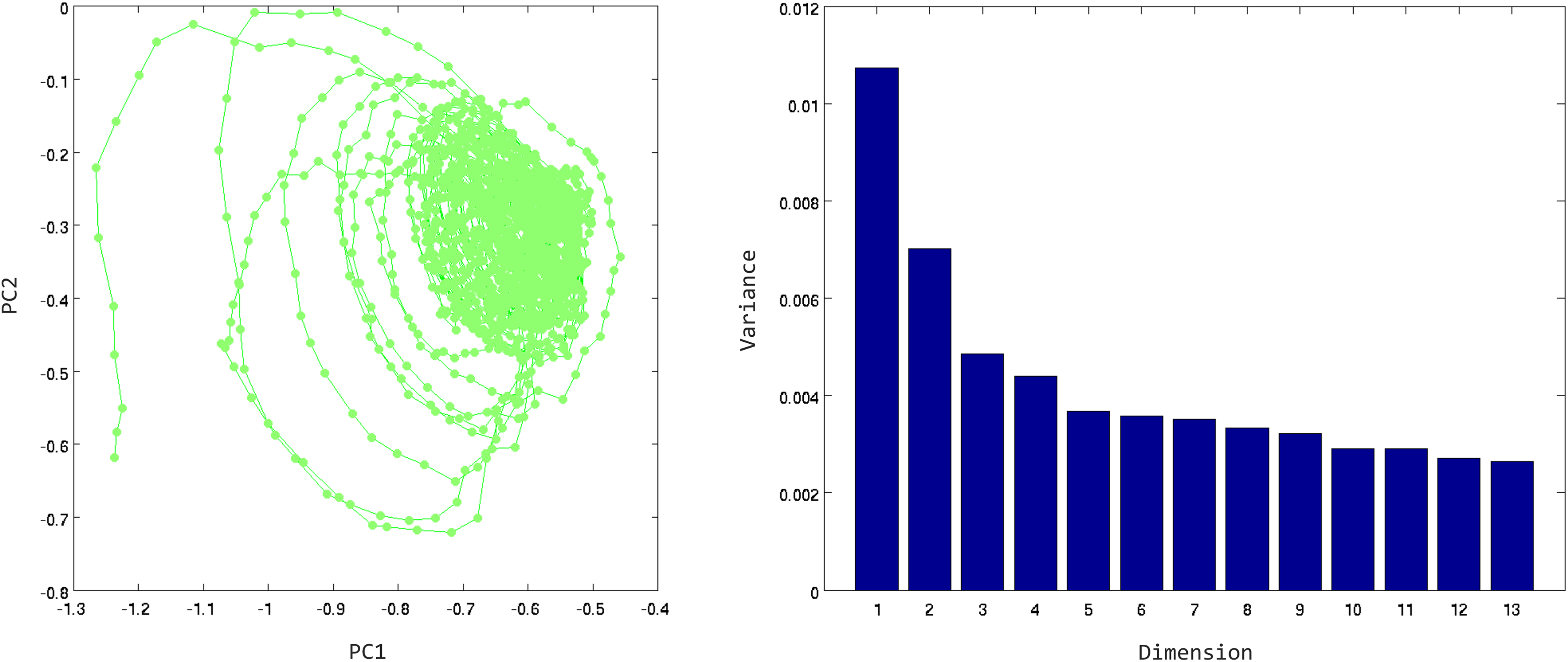
Tumba’s first two principal components (left) and first 13 eigenvalues (right) under a sliding window array.

The triple-quadruple hybridity we observed in the segundo and cascara is particularly prevalent in the tumba. Mean durations for the basic tumba pattern – which is played 77 times – are plotted in Figure 21’s top graph. The timing contour for the second half (notes 7–12) resembles the first (notes 1–6): a long-short-long group followed by a trio of relatively even notes. As the horizontal coordinates show, the long-short-long rhythm (notes 1–3 and 7–9) is not far from the quadruple-grid rhythm eighth-sixteenth-eighth, while the even group (notes 4–6 and 10–12) approximates “rushed” eighth-note triplets. A reason for the shortened eighth-notes and eighth-note triplets is that the rhythmic sequence just described – eighth-sixteenth-eighth plus three triplets – takes up more than a half-measure, leaving less space for the remaining three notes. The lower graph in Figure 21 shows how this mix of triple and quadruple durations is reflected in the placement of onsets along the measure cycle. While both halves of the pattern are generally more concordant with a triple grid (dashed coordinates), the “pull” toward quadruple (solid coordinates) is visible in almost all the notes.

Figure 21.

Top: Mean scaled interonset intervals (IOIs) for 77 iterations of the tumba pattern; horizontal coordinates give deadpan durations. Bottom: Mean location of onsets along the measures’ first half (notes 1–6) and second half (notes 7–12); vertical gridlines partition the half-measure into quadruple (solid) and triple (dashed) grids.

Recall that these are mean values. When all individual cases of the pattern are considered, the full scope of the tumba’s metric heterogeneity comes into view. Figure 22 unpacks the above mean values with PCA plots showing individual instances of each half of the basic tumba pattern, using a hand-curated measure window array that contains only the 77 instances of the unaltered pattern. Each point corresponds to the pattern’s first (left panel) or last (right panel) six notes. The location of points in relation to the three reference deadpan rhythms (x, y, z) indicates that triple and quadruple subdivision – as well as metrically blended patterns that lie between the deadpan regions – are present in the tumba’s timing.

Figure 22.

Tumba’s principal component analysis plots, using a measure window array of only those measures containing the unaltered pattern (n = 77). Panels correspond to the first (left) and second (right) halves of the 12-note pattern. Red points give the location of three reference deadpan rhythms.

Quinto

The quinto is the ensemble’s lead instrument. Like the tumba, it features a core pattern that undergoes extensive variation, causing the jumbled PCA plot shown in Figure 23. But while the tumba plays accompaniment (its frequent use of quiet strokes relegates it to the auditory background and its variants seldom depart dramatically from the main pattern), the quinto plays more energetically, befitting a soloistic foreground role. ²⁴ Not only does the quinto play accented patterns more often, but the distribution of these accents within the measure cycle is more varied, too. Figure 24 plots amplitude data within the measure cycle for all onsets (including variations) in the three congas. ²⁵ The segundo traces a clear phrasing contour, beginning quietly and crescendoing into beat 3’s two accented strokes before decreasing to its lowest value at the end of beat 1. The tumba is more diffused but still outlines a discernible amplitude profile where the most accented moment is the end of beat 1 and the least accented is the middle of beat 3. In the quinto, the metric span is saturated by a wide dynamic range; loud and quiet notes can occur just about anywhere within the measure. These graphs demonstrate that the three congas’ contrasting degrees of variance in the time domain parallel that in the amplitude domain.

Figure 23.

Quinto’s first two principal components (left) and first 13 eigenvalues (right) under a sliding window array.

Figure 24.

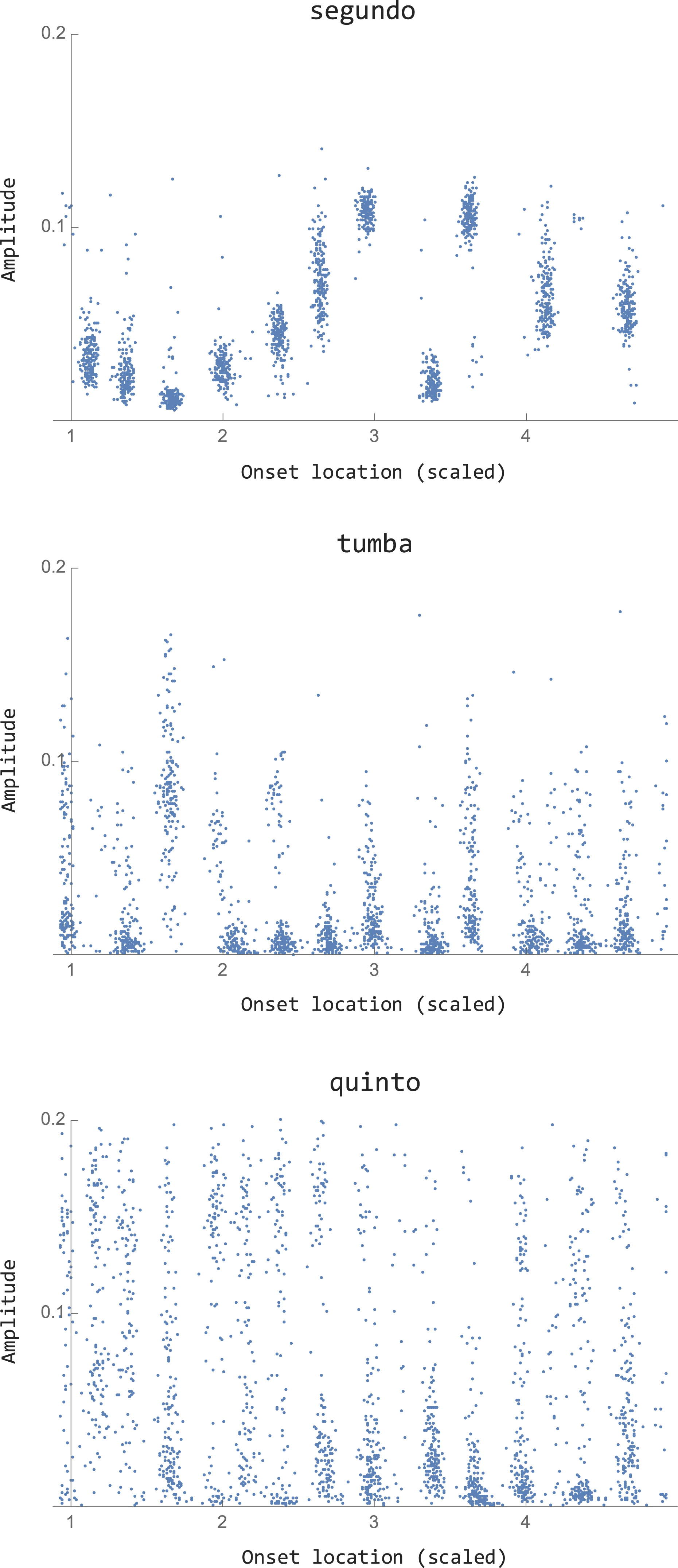
Amplitude values within the four-beat measure cycle for all onsets in the segundo, tumba, and quinto. Of the three instruments, the segundo has the most consistent amplitude contour.

A core quinto pattern emerges once we strip away the frequent rhythmic variation. Heard only 19 times in intact form, this pattern is often subjected to “modular” alterations that are constrained within any one of the pattern’s four beats. For instance, as illustrated from top to bottom in Figure 25, only the second and fourth beats might be substituted by variant modules; or only the first and second; or all except the third; or only the fourth. ²⁶ Note that we consider a change in accentuation (as in measure 68’s fourth beat) to be a rhythmic variant; the reason is that shifts in dynamics often co-occur with small shifts in timing, even if the notated rhythm appears unchanged. These substitutions illustrate what Crook (1982, p. 101) calls the “dialectic between fixed structure and freedom [that] lies at the core of the [quinto’s] improvisational process”.

Figure 25.

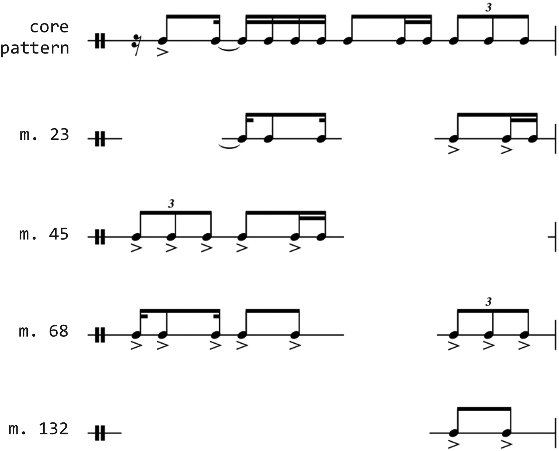
Examples of localized (within-beat) substitutions in the quinto. Blank spaces in each variation indicate no change from the core pattern.

The musical effect of the modular substitution process is one of almost continuous novelty without completely effacing the underlying theme. Since some of the substitutions involve a change in the number of notes, assessing within-beat variation quantitatively requires a method that uses many-to-many distances. We therefore sectioned each of the measure’s four beats into 20 bins, roughly equivalent – given tempo fluctuations – to non-overlapping windows of 20 ms. Doing so provided enough resolution to capture small timing differences while still being sufficiently coarse to highlight any clustering. Each bin was assigned either a 1 (onset) or a 0 (no onset) to form a binary sequence. This allowed us to assess within-beat variation by comparing all 186 instances of the same beat number (1, 2, 3, or 4) across measure cycles.

We used Toussaint’s (2013) “directed swap” algorithm – first outlined by Mäkinen (2001) for genome sequencing alignment – to calculate distances between the binary sequences. We then applied multidimensional scaling (MDS) to each beat’s distance matrix to produce the plots in Figure 26. Each notated rhythm corresponds to an approximate region of the plot, and points within that region are the particular performed rhythms – all basically notated the same, but having small differences in timing between them. In other words, a point connected to a notated example is an accurate representative of that rhythm but does not signify a unique location for it. Rather, points associated with a given notated rhythm are located in a general area of the graph that includes nearly identical instantiations of that rhythm. Where multiple links to one rhythm are displayed, these give a visual sense of the extent of the region. (For instance, the rhythm in beat 1’s upper left is linked to just two points but nearby smaller points also represent the same rhythm.) The region boundaries are fuzzy, in the sense that they are dependent on the particular perceptual biases of different listeners as well as on local rhythmic context (Desain & Honing, 2003).

Figure 26.

Multidimensional scaling plots showing within-beat variation in the quinto. Each point is marked with a circle whose size denotes the number of equal rhythms at that coordinate. The symbols ← and → denote, respectively, slightly early or slightly late note onsets with respect to the music notation.

The distribution of points shows which rhythms the performer favors given the infinite collection of possible rhythms. The higher clustering density in the two bottom graphs indicates that the quinto’s improvisatory excursions tend to happen in the first half of the measure: beats 3 and 4 are subject to less variation than beats 1 and 2. Beat 1’s two most frequent rhythms differ markedly, and other distinct rhythms appear with some frequency as well. Comparable scatter is visible in beat 2’s graph. In the case of beat 3, however, most rhythms are some version of either a triplet with a slightly late middle note, or a slightly shortened eighth-note plus two sixteenth-notes – two highly similar figures to begin with.

Conclusion

Describing the nature of periodicity across musical styles, Tenzer (2006, p. 22) notes that “virtually any musical element can create a sense of stability through return or constancy, and such stability will always be in dynamic dialog with change”. The above analyses delve into one such dialogue by revealing elements of novelty, change, and process inherent in an expert performance of Afro-Cuban rumba. We demonstrate that a simple binary paradigm of “theme” and “variation” does not hold within this particular performance. For most of the parts, a sense of stability emerges through a constant dialogue with change. Especially in the case of the quinto, we find that freedoms are often expressed by challenging the overall metric scheme while remaining within it. That is, the ground of restraint is instrumentalized for realizing the figure of freedom, a structure common to many African-diasporic musics (Chernoff, 1979; Gerstin, 2017; Locke, 2011; Racanelli, 2012).

In each of the parts, some of the variation appears to emerge from the dynamic superposition, rather than mutually exclusive alternation, of ternary and quaternary rhythmic states. This is not a case of straightforward polymeter distributed between different parts, where some parts locked into a stable ternary state exist alongside other parts locked into a stable quaternary state. Rather, while the clave leans toward a ternary state, and the segundo toward a quaternary state, the actual cumulative onsets of all five instruments display a significantly more complex reality. We propose that the superposition of quaternary and ternary states is the background or starting point from which the phenomenal rhythms emerge for all five parts in the ensemble, and that each player engages with this superposition in a unique way. The cumulative empirical measures of onsets over the entire performance illustrate the shape of the superposition itself, a well of possibility from which both theme and variations are actualized.

While we have limited our investigation in this article to the measurement and representation of onsets performed in a single recording, the data suggest interesting possibilities for perceptual research. In the spirit of inspiring future investigations, here we briefly speculate on some of the perceptual mechanisms that may be entailed in this performance. Pressing (1983, p. 52) describes the “perceptual multistability” through which performers and listeners engage in a constantly alternating gestalt flip between straightforward ternary and quaternary feels. While London maintains that “on a given perceptual occasion a musical figure can be metrically construed in only one way” (2012, p. 75), both Locke (2011, p. 55) and Stover (2009, pp. 131–132) argue that such a perceptual simultaneity is indeed possible. Our empirical evidence supports the latter view and appears to go even further. It is difficult to imagine how the performed onsets could occupy such a complex rhythmic space if the performer could only construe the event in either a straightforward ternary or quaternary way. Further, at certain points in the performance the very richness of onset timings – which display a high level of temporal complexity within a single cycle (or even beat) – suggests that they emerge from a deep blend of ternary and quaternary states rather than as conceptually segregated rhythmic dimensions. It is our sense, purely speculative at this point, that expert performers of Afro-Cuban rumba are capable of shifting between “superposition” and “gestalt” modes of perception/performance.

We also show that the clave, segundo, and non-variation segments of the tumba follow recurring timing contours. Such recurrence recalls the kind of “systematic… deviations from mechanical regularity” that Bengtsson and Gabrielsson (1983, p. 30) observed in different musical genres decades ago. We suspect that the clave, segundo, and tumba players in the present recording timed their rhythms with little concern for how they differed or not from some mechanically regular meter. But it is significant that the recurring timing tendencies defining each instrument’s consistency do not appear to be based on a shared underlying framework. In other words, it is not the case that all three instruments shape the divisions of any given beat in the same way. Part of this individuality is intertwined with the fact that the three patterns differ markedly in their general characteristics: the clave is less active, the segundo has more uneven durations and is ostensibly quadruple, and the tumba has more even durations and is ostensibly triple. This kind of polyrhythmic texture, where the constituent parts differ not only in their pre-existing rhythmic structure but also in their individual timing tendencies, is unlike the Brazilian and Malian multi-part percussion textures analyzed – respectively – by Gerischer (2006) and Polak (2010). In those instances, a shared (and non-isochronous) timing framework appears to serve as the metric substrate, whereas here there appear to be multiple tendencies simultaneously in play.

This rhythmic richness often occurs at a level of rhythmic granularity below the representational threshold of standard Western notation. Although the temporal structure of the onsets in the performance does not follow a rigid pattern, the typical variability tends to be confined to a small number of dimensions. This intuition holds for relatively stable patterns, such as the clave and segundo, and under cases of more substantial improvisational variations, as exhibited by the cascara, tumba, and quinto. For the first four instruments, we quantified the variability using principal components, in which the dominant eigenvectors measure the most prominent changes across measure cycles. The PCA method constructs an ordered basis of eigenvectors (and associated eigenvalues) for the covariance matrix. In the case of the clave and segundo, there are essentially only two non-zero eigenvalues, meaning that most of the variation is confined to two dimensions. By contrast, the other eigenvalues are larger for the other instruments. This indicates that more dimensions are required to describe their patterns. In the case of the quinto, there is not a sharp cutoff after which the eigenvalues become zero, which implies that the variability is not well described by a decomposition into equal-length vectors. Indeed, this is precisely why a different analysis procedure – one that takes into account varying lengths of patterns to visualize the distinct classes of rhythmic variation – was required for the quinto.

While the concept of analyzing various windows of a signal can be traced back to radar signal processing developed in the 1950s and 1960s, the idea of studying time series generated by a dynamical system using sliding windows is more recent. Takens (1981) was the first to show that an otherwise hidden state space and its local degrees of freedom could be obtained by examining delayed copies of the signal. Since then, others – e.g., Chazal, Cohen-Steiner, and Lieutier (2009) – extended and refined Takens’s approach to include recovery under noisy conditions. The noise robustness of time delay embeddings permits them to capture the overall structure of the variability in the rhythms in our recording without being overwhelmed by incidental variations.

It is important to emphasize in closing that the analyzed performance should not be considered representative of Afro-Cuban drumming in general. Rather, our study highlights the temporal details of a particular performance by a particular ensemble whose own style may very well sound appreciably different in a different place and time. Nonetheless, recognizable features of this repertoire – especially the rhythmic variation of repeating patterns and the conflation of triple and quadruple grids – receive considerable attention here, paving the way for an increasingly in-depth assessment of this rhythmically complex musical tradition.