Sage Journals: Discover world-class research

Abstract

Recent studies suggest that rhythmic syncopation is a relevant predictor for groove. In order to validate these claims, a reliable measure of rhythmic syncopation is required. This article investigates whether a particular notation-based model for estimating syncopation in Western popular music drum patterns adequately predicts perceived syncopation. A listening experiment was carried out with 25 professional musicians. Six popular music drum patterns were presented to the participants in all 15 pairwise combinations, and the participants chose the pattern from each pair that was more syncopated (win), compared to the other pattern (lose). Perceived syncopation was defined as the proportion of wins for each stimulus. The experiment showed that the model works well in general, but that it overemphasises the weight of syncopes on weak metric positions. This exaggerates the syncopation value of one particular drum pattern and generally leads to inflated syncopation values in the upper syncopation range. In consequence, the fit between the model and perceived syncopation was poor, even when flexible logarithmic functions $(χ_{4}^{2} = 26.980$ , p < .001) or exponential approach functions ( $χ_{4}^{2} = 28.344$ , p < .001) were used to link the model predictions to perceived syncopation. The model was revised and a numeric optimisation process was carried out to improve its fit. The revised model produces syncopation estimates that have a linear relationship with the perceived syncopation measures and a good fit with the data ( $χ_{3}^{2} = 2.537$ , p = .469). However, this revised model is based on only six drum patterns that cover a very limited range of rhythmic phenomena. In order to create a general model of syncopation in popular music drum patterns, further modelling work is necessary that involves a larger number and a wider variety of patterns.

Keywords

Syncopation (from the Greek συγκοπή, “sudden loss of strength”, Liddell, Scott, Jones, & McKenzie, 1996, p. 1666) is a rhythmic phenomenon in metered music that occurs when a weak metric position is accentuated by a note onset, but no onset happens on the subsequent strong metric position (Fitch & Rosenfeld, 2007; Longuet-Higgins & Lee, 1984; Temperley, 1999). Syncopation may trigger a moment of surprise in a listener; it has been interpreted as a “class of violations of temporal expectation” (Huron, 2008, p. 297) and as a conflict between rhythm and meter (Kühn, 1982; London, 2004, p. 86; Randel, 1999, p. 652). Temperley (2010) defined syncopation from a probabilistic point of view as a rhythmic pattern that is “low in probability given the prevailing meter” (p. 371). Syncopation has been understood as a source of rhythmic complexity in music, along with cross-rhythm, polyrhythm, and offbeatness (Fitch & Rosenfeld, 2007; Pfleiderer, 2006, pp. 145–150).

Syncopation has recently been discussed as a relevant factor for creating groove in listeners. In music psychology, groove is understood as a pleasurable “urge to move in response to music” (Janata, Tomic, & Haberman, 2012, p. 54). The groove phenomenon as inception of entrainment (Clayton, 2012; Clayton, Will, & Sager, 2005) or sensori-motor synchronisation (Repp, 2005; Repp & Su, 2013) in human beings is one of the most fundamental effects of music (Madison, 2001).

To date, the influence of syncopation on groove has only partly been clarified. One study found that musicians introduced more syncopation into their music when they intended to increase groove in listeners (Madison & Sioros, 2014). Others reported that a moderate degree of syncopation was best for groove, while low and high degrees had a negative impact on groove (Sioros, Miron, Davies, Gouyon, & Madison, 2014; Witek, Clarke, Wallentin, Kringelbach, & Vuust, 2014). Another study found that participants synchronised their body movement more readily with low- and medium-syncopation music, than with highly syncopated music (Witek et al., 2017). Finally, a recent study on popular music drum patterns reports that syncopation is positively associated with groove in expert music listeners, but no effect was measured for non-musicians (Senn, Kilchenmann, Bechtold, & Hoesl, 2018).

In order to assess the effect of syncopation on groove, a measure is required that reliably predicts the strength of listeners’ experience of syncopation. Several concepts of syncopation and methods for measuring its intensity have been described in the past (Arom, 1991; Gómez, Melvin, & Toussaint, 2005; Toussaint, 2002).

Longuet-Higgins and Lee (1984) proposed a method for quantifying syncopation which has been widely discussed (Essens, 1995; Fitch & Rosenfeld, 2007; Gómez, Thul, & Toussaint, 2007; Sioros, Davies, & Guedes, 2018; Witek et al., 2014). This model (the so-called LHL model) offers an operational definition of syncopation on the basis of notated music. It presents a method to assign a weight to each occurrence of syncopation in a rhythm, and it expresses the overall syncopation of a rhythm as the sum of these weights. Fitch and Rosenfeld (2007) found that the LHL method predicts listeners’ subjective experience of syncopation quite successfully.

LHL was conceived to model syncopation in monophonic music only. But most real-world musical situations involve several voices forming a complex, multi-layered rhythmic pattern. Witek et al. (2014) (revised version: Witek, Clarke, Wallentin, Kringelbach, & Vuust, 2015) expanded on the LHL model in order to accommodate two rhythmic layers, namely the bass drum and the snare drum voices of a Western popular music drum set pattern. These two voices are arguably the most important sources of syncopation in this kind of drum pattern. The hi-hat voice as the third essential layer of popular music drumming (Baur, 2002; Fleet & Winter, 2014; Stewart, 2000; Tamlyn, 1998) most of the time provides a background of regular pulsation against which the syncopated rhythms of bass drum and snare drum take place.

A model like the one presented by Witek et al. (2014, Index of syncopation, see supporting information in Witek et al., 2015) is of great use for the study of popular music drum patterns and groove, if it can be shown that the model predictions agree with listeners’ subjective impressions of syncopation intensity.

This study presents a formal implementation of a model that largely reproduces Witek et al.’s method, but takes a few liberties (see subsection A formal model description, below). It further offers a validation of the implemented model and aims to achieve three goals:

The study establishes a ground truth on perceived syncopation of six reconstructed popular music drum patterns in a listening experiment.

It investigates the fit between the predictions of the implemented model and the experimental results.

If necessary, it proposes changes to the model in order to improve its fit with the ground truth.

Listening experiment: Empirical ground truth on perceived syncopation

Stimuli

Six popular music drum patterns of eight bars’ duration were chosen as a basis for the experiment’s stimuli (Table 1) from a corpus of 250 popular music drum patterns (Lucerne Groove Research Library, http://www.grooveresearch.ch) that had been collected by the authors and their colleagues.

Table 1.

Stimuli and Perceived syncopation with 95% confidence intervals (see also Figure 3).

Title	Drummer	Act	Year	Wins	Losses	Perceived syncopation (S_p)	95% CI of S_p
Billie Jean	Leon Chancler	Michael Jackson	1982	21	104	0.168	(0.075, 0.261)
Kashmir	John Bonham	Led Zeppelin	1974	33	92	0.264	(0.155, 0.373)
My father’s eyes	Steve Gadd	Eric Clapton	1997	51	74	0.408	(0.286, 0.530)
Hyperpower	Josh Freese	Nine Inch Nails	2006	77	48	0.616	(0.495, 0.737)
Whole lotta love	John Bonham	Led Zeppelin	1969	96	29	0.768	(0.663, 0.873)
I got the feelin’	Clyde Stubblefield	James Brown	1968	97	28	0.776	(0.673, 0.879)

The six patterns are typical representatives of Western popular music drumming in rock, funk, or pop style. On the original recordings, the patterns have been played by some of the most renowned drummers in popular music. The passages have been selected such that the drummer plays a regular, at least partly repetitive, pattern. No drum solos were chosen. The patterns have the same instrumentation as the stimuli investigated by Witek et al. (2014): in the selected passages, the drummers use the hi-hat, bass drum, and snare drum only. Also in accordance with Witek et al., the six patterns feature an eighth-note-based pulse on the hi-hat. We chose the patterns to show considerable variation in terms of snare and bass drum syncopation (see Table 3 below), ranging from the rhythmically simple “archetypical rock beat” (Tamlyn, 1998, p. 12) of “Billie Jean” (Leon Chancler/Michael Jackson) to the highly complex patterns of “I got the feelin’” (Clyde Stubblefield/James Brown) and “Whole lotta love” (John Bonham/Led Zeppelin). “Kashmir” (John Bonham/Led Zeppelin) was chosen as a wildcard: it obtained a medium syncopation value according to the implemented model, which (to us authors) appeared to overestimate the perceived level of syncopation.

The first author, a professional jazz drummer, transcribed the patterns by ear from the original recordings. The original hi-hat voice was replaced by a regular, monotonic sequence of eighth notes without syncopation, in line with the stimuli used by Witek et al. (2014). The six resulting drum patterns can be studied in Figures 1 and 2.

Figure 1.

Transcriptions of “Billie Jean”, “Kashmir”, and “My father’s eyes” snare drum and bass drum patterns. Regular eighth-note sequences replace the original hi-hat voice.

Figure 2.

Transcriptions of “Hyperpower”, “Whole lotta love”, and “I got the feelin’” snare drum and bass drum patterns. Regular eighth-note sequences replace the original hi-hat voice.

The drum patterns were reconstructed in Avid ProTools (version 12.1) using audio samples from the Toontrack Superior Drummer (version 2.4.4) Custom & Vintage Library. One drum kit with a relatively neutral sound was chosen for the reconstruction of all six patterns, and a small amount of reverberation was added to the sound. This created the illusion that all drum patterns were played on the same drum kit in the same room.

Participants

Participants for the listening experiment were recruited within the first author’s personal and professional network. All participants were required to have completed a Bachelor of Arts in Music degree; most of them held a Master of Arts in Music degree. This ensured that participants were familiar with the concept of syncopation, theoretically and practically. A total of 25 participants (7 female, 17 male, age 28 ± 3.8 years) fulfilled this condition and took the test, which was carried out in German. Three people indicated they were non-native German speakers, but they claimed to have a good understanding of the language.

Setup and procedure

The listening experiment was carried out in several quiet environments at the Lucerne School of Music or at private indoor locations, supervised by the first author. Music examples were played from an Apple laptop computer (running Mac OS, version 10.11.6) using iTunes (version 12.7.2.60) for music playback. Participants brought their own headphones to the experiment; all participants used earbuds. Participants gave spoken feedback, which the researcher noted in an Excel for Mac (version 14.7.7) spreadsheet. Participants did not see the computer screen during the experiment.

Participants gave informed consent, and answered questions about their person. They listened to a test stimulus (similar to the experimental stimuli), and playback loudness was adjusted to a comfortably loud level. Playback loudness remained the same throughout the experiment. Participants were informed of their task, which consisted of listening to two drum patterns in each trial and of deciding which of the two was “more syncopated” (German: “synkopierter”) than the other. A test trial with two test stimuli was carried out, and participants had the opportunity to ask questions if they were not sure about their task. If participants asked about the meaning of “more syncopated”, they were advised to trust their instincts.

All 15 pairwise combinations of the six experimental stimuli were presented to the participants in a randomised order. The presentation order of the two stimuli within each trial was also randomly determined. For each pair, participants decided which of the two stimuli they perceived as “more syncopated”. Hence every trial was a Bernoulli experiment, and the outcome variable of the experiment is a count of wins (“more syncopated”) and losses (“less syncopated”) for each of the stimuli (Table 1).

The method of pairwise comparisons was the main reason that only six stimuli were used in the experiment. With six stimuli, each participant needed to carry out 15 comparisons. The total number of comparisons grows substantially with every additional stimulus, and we judged that carrying out more than 15 comparisons would exhaust participants’ patience.

Results and discussion

Perceived syncopation (S_p) is defined to be the true population proportion of wins for each of the stimuli. This parameter is estimated for each stimulus by its maximum likelihood estimator, the sample proportion of wins.

The experiment has a paired comparisons design with complete repetitions (Bramley, 2007; David, 1988; Wilkinson, 1957). Inference is based on the log-likelihood ratio (Casella & Berger, 2002; Kent, 1982; Wilks, 1938). The overall significance level is set to α = 0.05.

Estimates of Perceived syncopation (S_p) for each stimulus can be studied in Figure 3. We carried out an omnibus significance test against the null hypothesis that all stimuli had equal Perceived syncopation. The test offers very strong evidence that Perceived syncopation differs across the six stimuli ( $χ_{5}^{2} = 89.158$ , p < .001). Post hoc pairwise comparisons of Perceived syncopation between the six stimuli can be studied in Table 2. In order to control familywise type I error, Šidàk correction was applied (Sidàk, 1967; see also Huberty & Morris, 1989; Moskvina & Schmidt, 2008): probabilities are considered to be significant if they do not exceed $α_{S} = 0.0034.$

Figure 3.

Perceived syncopation (S_p) of the six stimuli. Error bars represent 95% confidence intervals for the estimate S_p (for data, see Table 1).

Table 2.

Pairwise comparisons of Perceived syncopation across stimuli (significance probabilities).

	Billie	Kashmir	Father	Hyper.	Whole
Kash.	0.191
Father	0.003	0.087
Hyper.	< 0.001	< 0.001	0.020
Whole	< 0.001	< 0.001	< 0.001	0.065
Feelin’	< 0.001	< 0.001	< 0.001	0.051	0.915

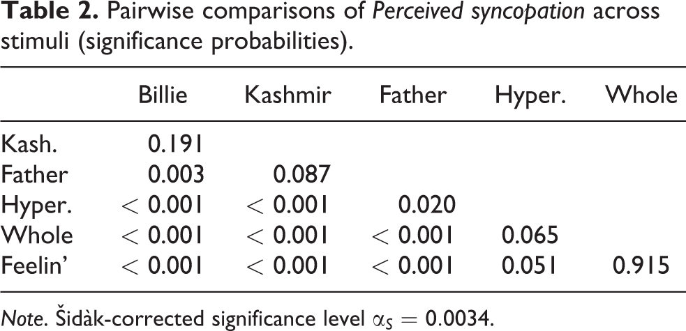
Note. Šidàk-corrected significance level $α_{S} = 0.0034$ .

Figure 3 shows that the stimuli are quite evenly spread across the range of Perceived syncopation. The ordering of the stimuli agrees with most of our expectations. However, we were expecting that the “Whole lotta love” pattern would be perceived to be more syncopated than the drum pattern of “I got the feelin’”. Judging from the participants’ responses, the listeners were undecided as to which of the two they found to be more syncopated. Also, we were surprised to find that the “Billie Jean” pattern (the “archetypical rock beat”) obtained 21 wins (Table 1). We expected this most generic of popular music patterns to never win against any of the other patterns in the sample.

The stimuli differed considerably in terms of Tempo (see Figures 1 and 2). The slowest pattern: “Kashmir” had a tempo of 82 bpm, whereas the fastest pattern, “I Got The Feelin’”, moved at 126 bpm. However, Tempo and Perceived syncopation were not significantly correlated (r = 0.115, p = 0.892), and hence we ruled out Tempo as a potentially confounding variable.

Modelling rhythmic syncopation in popular music drum patterns

The syncopation model by Witek et al. (2014)

Witek et al. (2014) (revised in Witek et al., 2015) presented a method to estimate the quantity of syncopation in the snare drum and bass drum voices of popular music drum patterns. They developed their method in a supporting text annexed to the main article. The general idea and the main steps of their method to quantify syncopation (which is based on the notated drum pattern and inherits many properties from the monophonic LHL model of Longuet-Higgins and Lee, 1984) can be described as follows:

Assign a metric weight to each metric position in a bar. Onbeat positions have a higher metric weight than offbeat positions. Metric weights for the 4/4 common time bar with the smallest subdivisions on the 16th-note level are shown in Figure 4. Note that Witek et al. (2014) slightly depart from the principle that each lower metric level (and hence the next lower metric weight) is reached by strict binary subdivisions: the third quarter-note beat of a bar has the same weight as the second and the fourth beat (for comparison, see Lerdahl & Jackendoff, 1983, p. 23; London, 2004, p. 41; Temperley, 2010, p. 357; Toussaint, 2013, p. 69).

Determine whether syncopation happens at a certain position. Syncopation occurs when in one rhythmic layer (either the snare drum or the bass drum) a note precedes a rest, and the rest is on a metric position with higher or equal weight compared to the note. Let us call the preceding note the syncopator, and the position with the rest is called the syncope (this terminology is newly introduced here). Examples of syncopation can be studied in Figure 5. In case (A), the bass drum note on the fourth 16th note (syncopator) has weight $w_{4} = - 3$ , and the subsequent rest appears on a quarter note with weight $w_{5} = - 1$ (syncope). Because w₄ is smaller than w₅, and because there is a note on w₄ and a rest on w₅, this qualifies as syncopation.

Establish the metric and instrumental weights of the syncopation. The metric weight of the syncopation is calculated as the difference between the metric weights of the syncope and the syncopator. In case (A), the bass drum note on the fourth 16th note (syncopator) has weight $w_{4} = - 3$ , and the subsequent rest appears on a quarter note with weight $w_{5} = - 1$ (syncope). The metric weight of the syncopation is $w_{5} - w_{4} = - 1 - (- 3) = 2$ . The model assigns instrumental weights according to the instrument the syncopation occurs on. Bass drum syncopation is given an instrumental weight of 2, snare drum syncopation obtains a weight of 1. Witek et al. (2014) support their choice of instrumental weights with arguments from cognitive theory. If a rest appears on the syncope in both the snare and the bass drum (“two-stream” syncopation), the instrumental weight is five. Syncopations (A) and (B) in Figure 5 have an instrumental weight of 2 (bass drum), (D) has an instrumental weight of 1 (snare drum), and (B) has instrumental weight 5 (“two stream”).

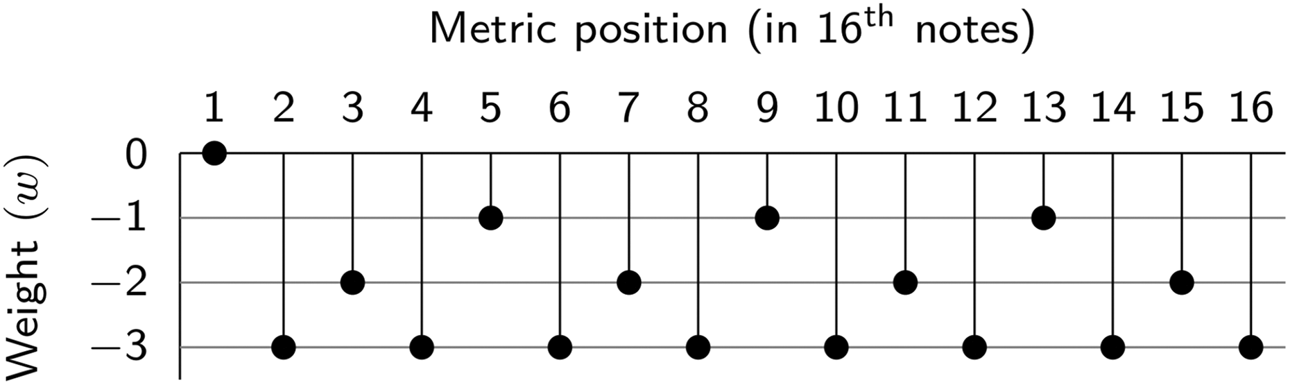
Add up all metric and instrumental weights across the pattern. Syncopation (A) in Figure 5 has a syncopation value of $2 + 2 = 4$ , (B) has a value of $1 + 5 = 6$ , (C) has value of $1 + 2 = 3$ , and (D) has value of $1 + 1 = 2$ . The entire pattern has model syncopation value of $4 + 6 + 3 + 2 = 15$ .

Figure 4.

Weight (w) per metric position for a common time bar according to Witek et al. (2014). The downbeat (1) weighs w = 0. For the remaining quarter notes (5, 9, 13) w = −1, offbeat eighth notes w = −2, and 16th notes w = −3.

Figure 5.

Examples of syncopation. (A) and (C) bass drum syncopation; (D) snare drum syncopation; (B) two-stream syncopation with snare drum syncopator.

Two side notes seem to be appropriate at this point: first, the Witek et al. model with the specification of metrical weights as shown in Figure 4 applies to 4/4 common time drum patterns only. Other meters (such as 12/8 or 3/4) are not explicitly considered. Second, the drum patterns investigated in this study only show syncopation on the tactus (quarter-note beats) and subtactus levels. Syncopation on higher levels (hyperbeats), as described by some theories on “metrical dissonance” (e.g., Krebs, 1987, 1999), appear to be irrelevant in this context.

A formal model description

In explaining their method, Witek et al. (2015) use little mathematical notation. In this section, we restate the core of their method in a more formal way. This allows us to program algorithms for calculating syncopation values and for more easily modifying the model parameters, if necessary.

Our implementation takes a few liberties in order to simplify the model presented originally in Witek et al. (2014) and Witek et al. (2015). This concerns the following aspects:

In Witek et al.’s (2015) model (Index of syncopation, p. 1), the metric weight of the syncope must be either greater than or equal to the weight of the syncopator for syncopation to happen. In our implementation, the metric weight of the syncope must be strictly greater than the weight of the syncopator. This choice leads to improved model fit, and it avoids overestimation of syncopation in simple patterns such as “Billie Jean”.

Witek et al. (2015) (Index of syncopation, p. 2) describe a rare situation, for which they conclude that the pattern of the hi-hat modifies the weight of a “two-stream” syncopation. We do not observe this configuration in our stimuli, so we omit it in the model.

Given these discrepancies, our model is not a strict implementation of the method proposed by Witek et al. (2015). Model syncopation values will differ when calculated by both methods. Nevertheless, our implementation builds largely on Witek et al.’s work, and we hope it captures the essential ideas of their method.

The modelling is carried out in four steps:

We determine the position of the potential syncopator for each potential syncope in the pattern.

We evaluate whether syncopation actually takes place between a potential syncopator and a potential syncope.

We attribute a weight to the syncopation.

We sum the weights of each occurrence of syncopation and evaluate the overall model syncopation of a pattern.

These four steps are elaborated in the paragraphs below.

Step 1

The drum pattern presented in Figure 5 (P, say) can be represented in matrix form as shown in Equation 1. Each column of P represents one metric position, and each row represents the pattern of one instrument: the row vector s represents the pattern in the snare drum voice, and b the pattern of the bass drum voice. When an onset occurs in a certain instrument at a certain metric position, the respective element takes value 1; when no onset occurs, the element takes value 0. The metric weights are represented in row vector w .

P = [\begin{matrix} s \\ b \\ w \end{matrix}] = [\begin{array}{r} 0 & 0 & 0 & 0 & 1 & 1 & 0 & 0 & 1 & 0 & 1 & 0 & 1 & 0 & 0 & 0 & 0 \\ 1 & 0 & 1 & 1 & 0 & 0 & 0 & 0 & 0 & 1 & 0 & 0 & 0 & 0 & 0 & 0 & 1 \\ 0 & - 3 & - 2 & - 3 & - 1 & - 3 & - 2 & - 3 & - 1 & - 3 & - 2 & - 3 & - 1 & - 3 & - 3 & - 3 & 0 \end{array}]

ϕ (a, w, i) = {\begin{array}{l} i - 1 - \sum_{j = 2}^{i - 1} [(j - 1) \prod_{k = 1}^{j} (δ (a_{i - j}, a_{i - k}) δ (w_{i - j}, w_{i - k}))] & if i > 2, \\ i - 1 & otherwise . \end{array}

We assume that all positions in the pattern, except for the first (because it is preceded by none), are potential syncopes. In the first step, we determine which of the metric positions that precede a potential syncope is the candidate syncopator that might trigger syncopation on the syncope. In order to express the rules for the candidate syncopator mathematically, we start by defining the δ function as a tool to create logical switches. It will prove to be useful throughout the entire modelling effort. Let u and v be two real numbers, then

δ (u, v) = {\begin{array}{l} 1, & if u > v \\ 0 & otherwise . \end{array}

The rule to find the candidate syncopator is given by the ϕ function in Equation 2. It takes three arguments:

a , the rhythmic pattern of one instrument (in our case, this can be either the snare drum row vector s , or the vector with the bass drum pattern b ),

w , the vector of metric weights,

and i, which is the metric position of the potential syncope (i > 1, $i \in ℕ$ ).

The ϕ function (Equation 2) looks complicated at a first glance, but it does a conceptually simple thing: for each potential syncope on position i in the pattern vector of one instrument, ϕ returns the candidate syncopator. This is the last position preceding the potential syncope:

that is marked by a note onset, while all subsequent metric positions up to the syncope are silent, and

that has a greater metric weight than all subsequent positions up to the syncope.

The first condition implements the fact that only the last note preceding a syncope can be a candidate syncopator. And the second condition makes sure that ϕ returns the candidate syncopator of the syncope on position i, instead of a syncope on an earlier position. If none of the positions up to i − 1 qualifies as a candidate syncopator, ϕ returns position i − 1 per default.

The ϕ function works for any kind of meter (respectively, for any kind of metric weight vector). For the common time 4/4 bar with 16th-note subdivisions, Witek et al. (2015) specify four different metric weights ( $0, - 1, - 2, - 3$ ) that are patterned as shown in Figure 4 and Equation (1). Given the metric weights of Figure 4, the syncopator can only be on three positions relative to the syncope: it is either the metric position preceding the syncope by one 16th, by one eighth or by one quarter note. The syncopator can never be three 16ths ahead of the syncope, because if the syncopator’s metric weight is smaller than the weight of the syncope, it is also smaller than the metric weight of a position two 16ths ahead of the syncope and, consequently, the syncopator would syncopate this other position.

In the common time metric environment, the output of the ϕ function reduces to the following rules:

Metric position i − 2 is the candidate syncopator, if the instrument a has an onset on $a_{i - 2}$ , but not on $a_{i - 1}$ , and if the metric weight $w_{i - 2}$ is greater than $w_{i - 1}$ .

Metric position i − 4 is the candidate syncopator, if there is an onset on $a_{i - 4}$ , but no onsets on $a_{i - 1}$ through $a_{i - 3}$ , and if $w_{i - 4}$ is the largest metric weight of $w_{i - 1}$ through $w_{i - 3}$ .

Position i − 1 is the default candidate syncopator, otherwise (regardless of the values of $a_{i - 1}$ and $w_{i - 1}$ ).

Step 2

Now that the candidate syncopes and their respective candidate syncopators have been determined, we will evaluate in a second step whether syncopation actually takes place in a specific situation. Syncopation occurs when the syncopator is marked by an onset and has a lower metric weight than the syncope, which is not marked by an onset. (Note that this rule differs from the one used by both Longuet-Higgins & Lee, 1984, and Witek et al., 2015, according to which syncopation happens when the metric weight of the syncopator is less than or equal to the syncope’s metric weight.)

The definition can be formalised as follows: Let i be the metric position of the syncope in instrument a (which can be the snare drum s or the bass drum b ), and j the position of the respective syncopator. Then the value of the syncopation switch function I_a at i is given by

I_{a, i} (a, w, i, j) = δ (w_{i}, w_{j}) δ (a_{j}, a_{i}),

where the δ function has the meaning defined in Equation 3. The value of $I_{a, i}$ is 1 when the metric weight of the syncope ( w _i) is greater than the weight of the syncopator ( w _j), and when the syncopator has an onset ( $a_{j} = 1$ ), while the syncope is silent ( $a_{i} = 0$ ). Thus, $I_{a, i}$ , as defined in Equation 4, returns 1 when syncopation occurs, and 0 otherwise.

Step 3

The third step is to assign a specific syncopation weight to each occurrence of syncopation. According to the Witek et al. (2015) model, the syncopation weight depends on the difference between the metric weights of the syncope and the syncopator (metric syncopation weight), on the instrument in which the syncopation happens (instrumental syncopation weight), and on whether the other instrument has an onset on the syncope or not (“two-stream” syncopation).

For the snare drum, the model proposes the following procedure to calculate the weight of a syncopation, W_s:

W_{s, i} (s, b, w, i, j) = w_{i} - w_{j} + 1 + 4 δ (1, s_{i} + b_{i}) .

This weight adds up several summands:

The difference between the metric weights of the syncope w _i and the syncopator w _j. If a position with a large metrical weight (e.g., the downbeat) is syncopated from a metrically light position (e.g., an off-eighth 16th note), this difference term has a large value.

For the snare drum, an instrumental weight of 1 is added.

Another weight of 4 is added in the two-stream syncopation case, when neither the snare drum, nor the bass drum have an onset on the syncope (this last condition is implemented by the $δ (1, s_{i} + b_{i})$ expression). Together, the weights of 1 and 4 add up to 5, which is the instrument weight for two-stream syncopation.

For syncopation on the bass drum at position i, the model proposes the following weights:

W_{b, i} (b, s, w, i, j) = w_{i} - w_{j} + 2 + 3 δ (1, s_{i} + b_{i}) .

Based on a perceptual argument, Witek et al. (2014) consider syncopation on the bass drum to have a greater impact on perception than syncopation on the snare drum. The instrumental weight is 2 for syncopation on the bass drum (compared to 1 for the snare drum). A weight of 3 is added in the case of two-stream syncopation. As a consequence, two-stream syncopations triggered by syncopators in either the snare drum or the bass drum have the same instrumental weight, namely 5.

Witek et al. (2015) do not seem to discuss the situation when a two-stream syncopation is simultaneously triggered by syncopators in both the snare drum and the bass drum. Several occurrences of this situation can be observed in the transcriptions of Figure 2: for example, the syncope on the last quarter note of bar 1 in “Whole lotta love” is initiated by syncopators in both the snare drum and the bass drum.

In our implementation of the model, we treat this situation as a two-stream syncopation triggered by the syncopator on the bass drum, only. In order to discount the snare drum syncopation in this specific case, we use an inverted variant of the syncopation switch function. $I_{a, i}^{- 1}$ returns 0 when syncopation occurs in instrument a on position i, and 1 otherwise:

I_{a, i}^{- 1} (a, w, i, j) = δ (1, I_{a} (a, w, i, j)) .

Step 4

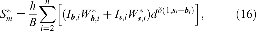
Finally, as a fourth step, we aggregate all components defined in Equations 4, 5, 6, and 7. Model syncopation (S_m) in the snare drum and bass drum voices of a popular music drum pattern with n metric positions is calculated as follows:

S_{m} = \sum_{i = 2}^{n} [I_{b, i} W_{b, i} + I_{s, i} W_{s, i} I_{b, i}^{- 1}]

where n is the number of metric positions in the pattern, $W_{b, i}$ is the syncopation weight at position i in the bass drum and $W_{s, i}$ is the syncopation weight at position i in the snare drum. The contribution of the bass drum at position i is the product of the syncopation switch function $I_{b, i}$ (1 if syncopation occurs, 0 otherwise) and the syncopation weight $W_{b, i}$ for the bass drum syncopation at i. The contribution of the snare drum is the product of the switch $I_{s, i}$ and the syncopation weight of the snare drum $W_{s, i}$ . $I_{b, i}^{- 1}$ multiplies the snare drum contribution by 0 if syncopation simultaneously occurs in the bass drum.

Total Model syncopation (S_m) is the sum of the syncopation contributions from the bass drum and snare drum across all n metric positions (except for the very first metric position at i = 1, which can never be a syncope). We implemented the model as a script in R. The Model syncopation (S_m) values of the six experimental stimuli can be inspected in Table 3.

Table 3.

Model fit: Logarithmic link function.

Title	S_p	S_m	${\tilde{S}}_{p}$	${\tilde{S}}_{p}^{°}$
Billie Jean	0.168	16	0.153	0.202
Kashmir	0.264	112	0.527	–
My father’s eyes	0.408	57	0.368	0.437
Hyperpower	0.616	104	0.509	0.577
Whole lotta love	0.768	290	0.785	0.840
I got the feelin’	0.776	170	0.637	0.701

Note. S_p, Perceived Syncopation; S_m, Model Syncopation; ${\tilde{S}}_{p}$ , fitted values all stimuli; ${\tilde{S}}_{p}^{o}$ , fitted values without “Kashmir”.

Fitting the model to the data

The model presented in the sections above quantifies syncopation on the basis of the notated drum pattern. In this section we investigate how reliably our implementation based on this model predicts the Perceived syncopation ground truth we established in the listening experiment. We consider the model to be successful if it is possible to find a link function that predicts Perceived syncopation from Model syncopation with adequate fit. This link function must be monotonically increasing (as Model syncopation increases, Perceived syncopation should also increase across the whole domain of the function).

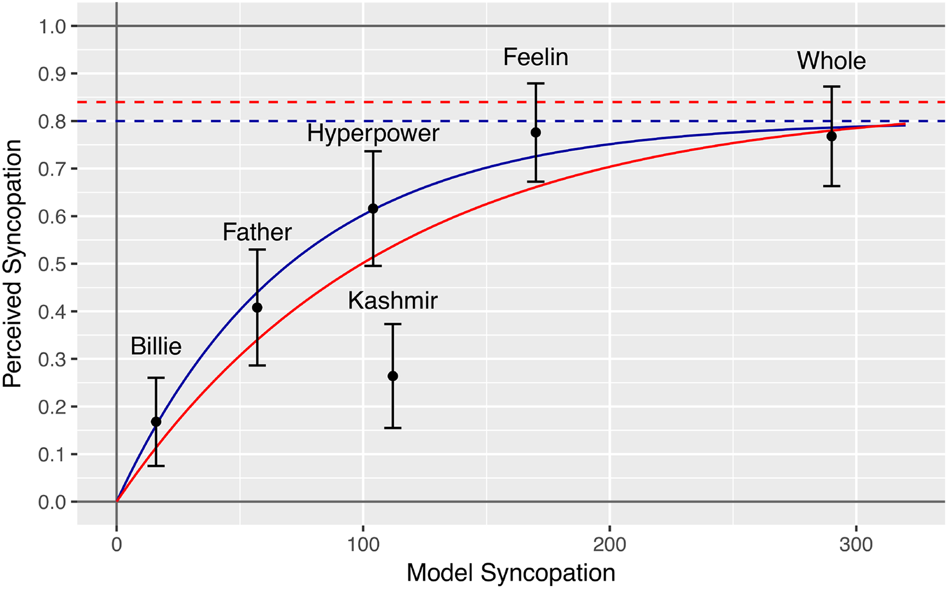
The link function does not necessarily have to be linear, any kind of increasing one-to-one function can prove to be useful. Also, we expect the link function to go through the origin: when there is no syncopation in the notation of a pattern ( $S_{m} = 0$ ), then the model should predict that this pattern always loses the pairwise comparison against patterns with more syncopation.

The relationship between the experimental data and the model can be studied in Figure 6. It plots Perceived syncopation (S_p) estimates for all six stimuli (including their 95% CI) against Model syncopation (S_m). The fitted values can be studied in Table 3.

Figure 6.

Logarithmic link function: Perceived syncopation (S_p) as a function of Model syncopation (S_m). The red curve is the best fit logarithmic function with all stimuli. The blue curve is the best fit function when “Kashmir” is omitted.

A log-based function might be a promising candidate for the link function: the relationship between Perceived syncopation (S_p) and Model syncopation (S_m), as seen in Figure 6, appears to flatten for higher values. In perception, the relationship between the physical intensity of a stimulus and the perceivers’ sensitivity to changes in intensity often shows a logarithmic relationship: in auditory perception, for example, perceived loudness is modelled as a logarithmic function of acoustical sound pressure (dB scale). Weber–Fechner’s Law is a generalisation of these frequently observed logarithmic relationships (MacKay, 1963; Masin, Zudini, & Antonelli, 2009).

The blue and red curves in Figure 6 are log-based link functions of Model syncopation (S_m) that return Estimated perceived syncopation ( ${\tilde{S}}_{p}$ ):

{\tilde{S}}_{p} = f_{log} (S_{m}) = q log (k S_{m} + 1), S_{m} \geq 0,

where q > 0 and k > 0 are scale and shape parameters, respectively. Parameters q and k are chosen such that the sum of the squared deviations between Perceived syncopation (S_p) and the fitted value on the curve, ${\tilde{S}}_{p}$ , are minimised. Note that function f_log passes through the origin, regardless of the choice of q and k.

The red curve in Figure 6 is the line of best fit using all six data points. This curve fits the data poorly ( $χ_{4}^{2} = 27.960$ , p < .001). The main reason for the poor fit appears to be the displacement of the “Kashmir” pattern. It can easily be shown that the “Kashmir” pattern is misplaced by the model: Perceived syncopation is greater in “Hyperpower” ( $S_{p} = 0.616$ ) than in “Kashmir” ( $S_{p} = 0.264$ ), and this difference is significant ( $χ_{1}^{2} = 16.084$ , p < .001). Yet Model syncopation is greater for “Kashmir ( $S_{m} = 112$ ) than for “Hyperpower” ( $S_{m} = 104$ ). With respect to these two stimuli, S_p cannot be expressed as a strictly increasing function of S_m.

The blue curve is the line of best fit when “Kashmir” is excluded, and only the five data points of the other stimuli are used. It is defined by

{\tilde{S}}_{p}^{o} = f_{log} (S_{m}) = 0.28 log (0.066 S_{m} + 1),

with q = 0.28 and k = 0.066. This function fits the data (without “Kashmir”) reasonably well ( $χ_{3}^{2} = 5.066$ , p = 0.167).

One theoretically problematic aspect is that the image space of f_log is the interval (0, ∞), whereas S_p is bounded within (0, 1). This, however, seems to be quite irrelevant in practice: f_log exceeds the interval (0, 1) when $S_{m} \approx 524$ . This is a score unlikely to occur in real-world popular music drum patterns of only eight bars’ duration.

Another potential functional link between S_m and ${\tilde{S}}_{p}$ can be defined as follows:

{\tilde{S}}_{p} = f_{exp} (S_{m}) = q (1 - e^{- k S_{m}}), S_{m} \geq 0,

where $q \in (0, 1)$ and k > 0. Functions of this form have frequently been called exponential approach or shifted exponential functions. These functions approach scale parameter q as $S_{m} \to \infty$ . And since $q \in (0, 1)$ , f_exp never exceeds 1 (thus avoiding the theoretical problem of the log-based link function). Again, k determines the shape of function f_exp, and the function passes through the origin, regardless of the choice of q and k.

The fit of the exponential approach functions can be studied in Figure 7 and Table 4. Again, the red curve shows that, if all stimuli are included, the fit is poor ( $χ_{4}^{2} = 28.691$ , p < .001). If “Kashmir” is omitted (blue curve), the function is given by

{\tilde{S}}_{p}^{°} = f_{exp} (S_{m}) = 0.80 (1 - e^{- 0.014 S_{m}}),

and it has a very good fit with the data ( $χ_{3}^{2} = 1.226$ , p = 0.747).

Figure 7.

Exponential approach link function: Perceived syncopation (S_p) as a function of Model syncopation (S_m). The red curve is the best fit exponential approach function with all stimuli. The blue curve is the best fit function when “Kashmir” is omitted. Dashed lines are the approach limits.

Table 4.

Model fit: Exponential approach link function.

Title	S_p	S_m	${\tilde{S}}_{p}$	${\tilde{S}}_{p}^{°}$
Billie Jean	0.168	16	0.114	0.161
Kashmir	0.264	112	0.537	–
My father’s eyes	0.408	57	0.340	0.440
Hyperpower	0.616	104	0.514	0.613
Whole lotta love	0.768	290	0.780	0.786
I got the feelin’	0.776	170	0.661	0.726

Note. S_p, Perceived Syncopation; S_m, Model Syncopation; ${\tilde{S}}_{p}$ , fitted values all stimuli; ${\tilde{S}}_{p}^{o}$ , fitted values without “Kashmir.”

In summary, our implementation of the syncopation model, based on the modelling work of Witek et al. (2015), solidly predicts how listeners perceived the degree of syncopation in four of the six stimuli used in the experiment. But the model overestimates the syncopation level of “Kashmir”, and it also seems to overstate the syncopation level of “Whole lotta love”. The model returns a large numerical difference between the Model syncopation values of “I got the feelin’” and “Whole lotta love”, but participants did not perceive such a difference.

The flexible logarithmic or exponential link functions approximate the distortion in the higher syncopation range fairly well, but the “Kashmir” pattern seems to be misplaced, regardless of the choice of link function.

Revising the model

In the remainder of this study, we modify the model in order to improve its fit with the experimental data. Particularly, we intend to avoid the misalignment of “Kashmir” and the exaggeration of differences in the upper syncopation range.

The study of the “Kashmir” pattern (Figure 1) shows that the greatest contribution to this stimulus’ Model syncopation (S_m) comes from the 16th notes in the bass drum just after beats one and three. These notes act as syncopators to the rests on the subsequent eighth-note positions. The weight of these syncopes is increased by the fact that the snare drum has a simultaneous rest, so the constellation is treated as a two-stream syncopation by the model.

Yet, participants do not seem to perceive the “Kashmir” pattern as particularly syncopated. Potentially, listeners heard the 16th notes as ornaments to the beats, rather than as syncopes. This effect might be increased by dynamics: the echoing 16ths in the “Kashmir” pattern are always softer than the note on the downbeat. Thus, we can describe the “Kashmir” pattern as an “archetypical rock beat” (Tamlyn, 1998, p. 12) like “Billie Jean” with a kind of “echo” on the bass drum beats. The model’s overestimation of syncopation in the “Kashmir” pattern seems to be linked to the metric weights and to the emphasis on two-stream syncopation as an important factor.

The distortion in the upper syncopation range can also be traced back to the fact that, in the “Whole lotta love” pattern, many syncopations happen on the eighth-note syncope level in both the bass drum and the snare drum. It is the sheer number of these syncopated events on a low metric level that inflates the S_m syncopation estimate for this pattern.

The “I got the feelin’” pattern, conversely, shows fewer syncopated events altogether, but a large proportion of them are two-stream syncopations and take place on high metric levels. Potentially, the distortion in the upper syncopation range above S_m = 150 can be avoided by adapting metric weights and the weight of two-stream syncopation.

We will use the mathematical model description presented above as a template to reformulate the syncopation model. Many components such as the ϕ function (Equation 2), the δ function (Equation 3), and the syncopation switch function $I_{a, i}$ (Equation 4) will be reused in this revision and remain defined as above.

Let the revised metric weight W* of a syncope at metric position i in instrument a be defined as follows:

W_{a, i}^{*} (a, w, i, j, c) = c^{w_{i}} - c^{w_{j}},

where $j = ϕ (a, w, i)$ is the metric position of the syncopator, and $c \geq 1$ is a parameter that needs to be estimated in a process of optimisation (description below).

The parameter c regulates the relative weight between metric positions. Recall that $w_{i} = 0$ for the downbeat, $w_{i} = - 1$ for all other quarter beats, $w_{i} = - 2$ for the offbeat eighth-note positions, and finally $w_{i} = - 3$ for the off-eighth, 16th-note positions (see Figure 4).

The revised weight of the downbeat is always $c^{0} = 1$ , regardless of the value of c. But the weight of all the other positions is reduced as c increases. For example, when c = 2, the downbeat has weight $2^{0} = 1$ , the secondary beats (beats two, three, and four of the bar) have weight $2^{- 1} = 1 / 2$ , offbeat eighths $2^{- 2} = 1 / 4$ , and off-eighth 16ths $2^{- 3} = 1 / 8$ . So, when c = 2, a syncope on a downbeat, triggered by the syncopator one 16th note ahead has weight

W_{a, i}^{*} = c^{w_{i}} - c^{w_{j}} {= 2}^{0} - 2^{- 3} = 1 - \frac{1}{8} = \frac{7}{8},

whereas a syncope on an offbeat eighth note, triggered by a syncopator one 16th note ahead only has weight

W_{a, i}^{*} = c^{w_{i}} - c^{w_{j}} {= 2}^{- 2} - 2^{- 3} = \frac{1}{4} - \frac{1}{8} = \frac{1}{8} .

Hence, large c will reduce the weights of the syncopes on the offbeat eighth notes of both “Kashmir” and “Whole lotta love”.

With the described amendment to the calculation of syncopation weight W*, the revised Model syncopation ( $S_{m}^{*}$ ) is calculated by

S_{m}^{*} = \frac{h}{B} \sum_{i = 2}^{n} [(I_{b, i} W_{b, i}^{*} + I_{s, i} W_{s, i}^{*}) d^{δ (1, s_{i} + b_{i})}],

where B is the number of beats in the pattern. By dividing the estimate by B we make it independent of pattern length, hence $S_{m}^{*}$ is Model syncopation per beat. The h coefficient is a scaling factor, which will be explained below. The expression $d^{δ (1, s_{i} + b_{i})}$ is the two-stream syncopation factor: it equals d when both instruments are silent on i (i.e., when two-stream syncopation happens), and 1 otherwise.

To summarise, two unknowns need to be estimated in order to optimise the model $S_{m}^{*}$ : c, which governs the relationship between metric weights, and d, the two-stream syncopation factor.

Fitting the revised model to the data

A numeric optimisation process was implemented in R, which aimed to minimise the root mean square error between the link function (which is separately fitted for each evaluated combination of c and d) and the experimental data. A linear function was chosen as the target link function between Perceived and Model syncopation. We also want the linear link function to go through the origin, such that ${\tilde{S}}_{p} = 0$ when $S_{m}^{*} = 0$ .

The root mean square error of the model was at a minimum when c = 2.8 and d = 1.6. Hence the revised model is given by

W_{a, i}^{*} (a, w, i, j {) = 2.8}^{w_{i}} - {2.8}^{w_{j}}

and

S_{m}^{*} = \frac{1.32}{32} \sum_{i = 2}^{129} [(I_{b, i} W_{b, i}^{*} + I_{s, i} W_{s, i}^{*}) {1.6}^{δ (1, s_{i} + b_{i})}] .

In the case of this study’s stimuli with eight bars, there are 32 quarter beats per stimulus, hence B = 32, and the number of metric positions in each pattern is n = 129 (the downbeat of the ninth bar is the last position in each pattern, see Figures 1 and 2).

The result of the revision and optimisation can be studied in Figure 8 and Table 5. The six data points follow a linear regression line quite closely. Every fitted value ${\tilde{S}}_{p}$ is within the 95% confidence interval of the corresponding perceived syncopation estimate S_p. The fit of the model with the data is good ( $χ_{3}^{2} = 2.908$ , p = 0.406).

Figure 8.

Perceived syncopation (S_p) as a function of the optimised Model syncopation ( $S_{m}^{*}$ ) measure. The red line is the best fit linear regression line.

Table 5.

Model fit: Optimised model.

Title	S_p	(95% CI of S_p)	$S_{m}^{} = {\tilde{S}}_{p}^{}$
Billie Jean	0.168	(0.075, 0.261)	0.212
Kashmir	0.264	(0.155, 0.373)	0.299
My father’s eyes	0.408	(0.286, 0.530)	0.343
Hyperpower	0.616	(0.495, 0.737)	0.604
Whole lotta love	0.768	(0.663, 0.873)	0.804
I got the feelin’	0.776	(0.673, 0.879)	0.758

Note. S_p, perceived syncopation; $S_{m}^{*}$ , revised model syncopation; ${\tilde{S}}_{p}^{*}$ , revised fitted values.

The scaling factor h = 1.32 was chosen such that the slope of the linear link function becomes 1. As a consequence of this scaling, the revised Model syncopation ( $S_{m}^{*}$ ) and revised Perceived syncopation estimate ( ${\tilde{S}}_{p}^{*}$ ) have the same range: $S_{m}^{*}, {\tilde{S}}_{p}^{*} \in (0, 1)$ .

The revision and optimisation improved two aspects of the original model with respect to this study’s six stimuli:

The misplacement of the “Kashmir” pattern has been fixed. In the revised model, this pattern is well aligned with the other stimuli.

Also, the original model predicted that the “Whole lotta love” pattern was much more syncopated than the “I got the feelin’” pattern, but the participants of the experiment did not perceive this difference. The revised model does not show this distortion.

Thanks to the equivalence between the revised Model syncopation ( $S_{m}^{*}$ ) and the estimated Perceived syncopation ( ${\tilde{S}}_{p}$ ), the model values are straightforward to interpret. The $S_{m}^{*}$ value estimates the probability that, in a listening experiment with paired comparisons, listeners perceive a drum pattern to be more syncopated than any other pattern randomly drawn from the population of Western popular music drum patterns.

The accuracy and general applicability of this estimate is difficult to assess at this moment. The estimate rests on data from a small experiment with only six drum patterns. And these patterns were not randomly chosen from the population of Western popular music drum patterns. Rather, they were selected to represent a wide range from weak to strong syncopation. Another choice of stimuli might result in a very different rule for $S_{m}^{*}$ .

A practical drawback of the revised model is that computations do not rely on integers only, as the original Witek et al. (2015) model did. Hence it is unwieldy to calculate $S_{m}^{*}$ by hand, and the use of a computer is recommended. An R script for calculating $S_{m}^{*}$ on the basis of a pattern matrix is provided in this article’s supplementary material section.

Conclusions

This study presented the implementation of a model for quantifying syncopation in popular music drum patterns, which was based on a method by Witek et al. (2014) (revised version: Witek et al., 2015). The implemented model was then empirically validated. Comparing the model predictions with the data from the listening experiment indicated that the model predicted Perceived syncopation quite well in general. However, our findings also showed that the model overemphasised some aspects of a rhythmic pattern linked to syncopation on weak metric positions, which led to inconsistencies between Perceived and Model syncopation.

We revised the model and improved its fit with the empirical data by numerical optimisation. We found model parameters such that the model expresses Perceived syncopation of the six stimuli as a linear function of Model syncopation.

For the time being, the revised model seems to be our best guess at estimating syncopation in popular music drum patterns, even though many questions remain unanswered. For example, the contribution of the hi-hat to syncopation has been assumed to be irrelevant in this study, yet there is no evidence so far that the contribution of the hi-hat is indeed negligible.

The model is based on a small-scale listening experiment with only six stimuli. A future experiment to validate and further improve the model should include more stimuli in order to better represent the diversity of popular music drum patterns and to generate more stable results. Also, the model should be expanded to include other instruments of the drum set and other time signatures than 4/4 common time.

The complete paired comparison design becomes impractical as the number of stimuli increases (each participant needs to perform “n choose 2” comparisons. Designs with incomplete repetitions might prove useful to solve this problem (Bramley, 2007; Silverstein & Farrell, 2001; Wilkinson, 1957), or methods in which participants rank the stimuli according to perceived syncopation (Bramley, 2005; Kendall & Gibbons, 1990).

In this study we assumed, in line with Longuet-Higgins and Lee (1984) and Witek et al. (2014), that syncopation can be quantified by summing up the weights of all syncopated events in a pattern. This hypothetical additive property of syncopation is somewhat questionable: syncopation is based on the notion of meter. The more syncopated events we introduce into a pattern, the less listeners will be aware of the meter, and the perceived syncopation effect will be weakened. Another problem with syncopation is that listeners with little musical expertise are unlikely to know the concept of syncopation (this was the main reason we recruited only musicians for the listening experiment).

It might be beneficial to replace the concept of syncopation by the concept of rhythmic complexity in the future, as suggested by Fitch and Rosenfeld (2007). Rhythmic complexity might be modelled using a predictive coding approach (Clark, 2013; Vuust, Dietz, Witek, & Kringelbach, 2018; Vuust & Witek, 2014). Increasing rhythmic complexity is associated with reducing listeners’ sense of, and orientation within, the meter. Potentially, complexity can more successfully be projected on a quantitative dimension than syncopation. More rhythmic complexity is likely to be associated with more metric confusion in the listener. Hence, a highly complicated rhythm may be perceived as complex, but it may not be perceived as syncopated, because the listener’s sense of the meter is too confused to distinguish between weak and strong metric positions.

Another potentially valuable metric to explore is beat strength, or, alternatively, perceptual beat salience: listeners with any degree of musical expertise will be able to answer the question whether they recognise the beat more easily in one or in another stimulus. Perceptual beat salience can be expected to be a reverse measure of syncopation or rhythmic complexity.

Supplemental Material

Supplemental Material, syncopation_model_180702 - Modelling perceived syncopation in popular music drum patterns: A preliminary study

Supplemental Material, syncopation_model_180702 for Modelling perceived syncopation in popular music drum patterns: A preliminary study by Florian Hoesl, and Olivier Senn in Music & Science

Footnotes

Acknowledgement

The authors would like to thank Lorenz Kilchenmann and Toni Bechtold for their support preparing the stimuli.

Contributorship

Designed the study: FH, OS. Prepared the stimuli: FH. Carried out the listening experiment: FH. Analysed the data: OS. Created the mathematical models: OS. Wrote the paper: OS, FH.

Declaration of conflicting interests

The authors declared no potential conflicts of interest with respect to the research, authorship, and/or publication of this article.

Funding

The author(s) disclosed receipt of the following financial support for the research, authorship, and/or publication of this article: This research was partly funded by the Swiss National Science Foundation (grant No. 100016 162504 to Olivier Senn).

Peer review

Justin London, Carleton College, Department of Music.

David Meredith, Aalborg University, Department of Architecture, Design and Media Technology.

Brian Bemman, Aalborg University, Department of Architecture, Design and Media Technology.

Supplemental Material

Supplemental material for this article is available online.

References

Arom

(1991). African polyphony and polyrhythm: Musical structure and methodology. Cambridge, England: Cambridge University Press.

Baur

(2002). Ringo ‘round Revolver: Rhythm, timbre, and tempo in rock drumming. In Reising

(Ed.), Every sound there is: The Beatles’ Revolver and the transformation of rock and roll (pp. 171–182). Aldershot, England: Ashgate.

Bramley

(2005). A rank-ordering method for equating tests by expert judgment. Journal of Applied Measurement, 6, 202–223.

Bramley

(2007). Paired comparison methods. In Newton

Baird

Goldstein

Patrick

Tymms

(Eds.), Techniques for monitoring the comparability of examination standards (pp. 246–294). London, England: Qualifications and Curriculum Authority.

Casella

Berger

R. L

. (2002). Statistical inference. Pacific Grove, CA: Duxbury. ISBN:978-0-534-24312-8

Clark

(2013). Whatever next? Predictive brains, situated agents, and the future of cognitive science. The Behavioral and Brain Sciences, 36(3), 181–204. doi:10.1017/S0140525X12000477

Clayton

(2012). What is entrainment? Definition and applications in musical research. Empirical Musicology Review, 7(1–2), http://hdl.handle.net/1811/52979.

Clayton

Will

Sager

(2005). In time with the music: The concept of entrainment and its significance for ethnomusicology. European Meetings in Ethnomusicology, 11, 3–142.

David

H. A

. (1988). The method of paired comparisons (2nd ed.). London, England: Hodder Arnold. ISBN:978-0-85264-290-0

10.

Essens

(1995). Structuring temporal sequences: Comparison of models and factors of complexity. Perception & Psychophysics, 57(4), 519–532. doi:10.3758/BF03213077

11.

Fitch

W. T.

Rosenfeld

A. J.

(2007). Perception and production of syncopated rhythms. Music Perception: An Interdisciplinary Journal, 25(1), 43–58. doi:10.1525/mp.2007.25.1.43

12.

Fleet

Winter

(2014). Investigating the origins of contemporary basics on the drum kit: An exploration of the role of the hi-hat in Anglo-American popular musics from 1960 until 1974. Popular Music, 33(2), 293–314. doi:10.1017/S0261143014000269

13.

Gómez

Melvin

Toussaint

G. T.

(2005). Mathematical measures of syncopation. In Proc. BRIDGES: Mathematical connections in art, music and science (pp. 73–84). Madrid, Spain: Escuela U. De Informática y Politécnica.

14.

Gómez

Thul

Toussaint

G. T.

(2007). An experimental comparison of formal measures of rhythmic syncopation. In International Computer Music Conference, 2007 (pp. 101–104). Copenhagen, Denmark: Michigan Publishing. Retrieved from http://hdl.handle.net/2027/spo.bbp2372.2007.023

15.

Huberty

C. J.

Morris

J. D.

(1989). Multivariate analysis versus multiple univariate analyses. Psychological Bulletin, 105(2), 302–308. doi:10.1037/0033-2909.105.2.302

16.

Huron

. (2008). Sweet anticipation: Music and the psychology of expectation. Cambridge, MA and London, England: MIT Press. ISBN:978-0-262-58278-0

17.

Janata

Tomic

S. T.

Haberman

J. M.

(2012). Sensorimotor coupling in music and the psychology of the groove. Journal of Experimental Psychology. General, 141(1), 54–75. doi:10.1037/a0024208

18.

Kendall

Gibbons

J. D

. (1990). Rank correlation methods (5th ed.). Oxford, England and New York, NY: Oxford University Press. ISBN:978-0-19-520837-5

19.

Kent

J. T.

(1982). Robust properties of likelihood ratio tests. Biometrika, 69(1), 19–27. doi:10.1093/biomet/69.1.19.

20.

Krebs

(1987). Some extensions of the concepts of metrical consonance and dissonance. Journal of Music Theory, 31(1), 99–120. doi:10.2307/843547

21.

Krebs

(1999). Fantasy pieces: Metrical dissonance in the music of Robert Schumann. Oxford, England: Oxford University Press. ISBN:978-0-19-535381-5

22.

Kuhn

(1982). Synkope. In Honegger

Massenkeil

(Eds.), Das grosse Lexikon der Musik (Vol. 8, pp. 66–67). Freiburg im Breisgau, Germany: Verlag Herder.

23.

Lerdahl

Jackendoff

. (1983). A generative theory of tonal music. Cambridge, MA: MIT Press. ISBN:978-0262-26091-6

24.

Liddell

H. G.

Scott

Jones

H. S.

McKenzie

(1996). A Greek–English lexicon. Oxford, England: Clarendon Press.

25.

London

(2004). Hearing in time: psychological aspects of musical meter. Oxford, England: Oxford University Press.

26.

Longuet-Higgins

H. C.

Lee

C. S.

(1984). The rhythmic interpretation of monophonic music. Music Perception: An Interdisciplinary Journal, 1(4), 424–441. doi:10.2307/40285271

27.

MacKay

D. M.

(1963). Psychophysics of perceived intensity: A theoretical basis for Fechner’s and Stevens’ laws. Science, 139(3560), 1213–1216. doi:10.1126/science.139.3560.1213-a

28.

Madison

(2001). Different kinds of groove in jazz and dance music as indicated by listeners’ ratings. In Proceedings of the VII International Symposium on Systematic and Comparative MusicologyIII International Conference on Cognitive Musicology (pp. 108–112). Jyväskylä, Finland: Department of Musicology, University of Jyväskylä.

29.

Madison

Sioros

(2014). What musicians do to induce the sensation of groove in simple and complex melodies, and how listeners perceive it. Frontiers in Psychology, 5. doi:10.3389/fpsyg.2014.00894

30.

Masin

S. C.

Zudini

Antonelli

(2009). Early alternative derivations of Fechner’s law. Journal of the History of the Behavioral Sciences, 45(1), 56–65. doi:10.1002/jhbs.20349

31.

Moskvina

Schmidt

K. M.

(2008). On multiple-testing correction in genome-wide association studies. Genetic Epidemiology, 32(6), 567–573. doi:10.1002/gepi.20331

32.

Pfleiderer

(2006). Rhythmus: Psychologische, theoretische und stilanalytische Aspekte populärer Musik. Bielefeld, Germany: Transcript Verlag.

33.

Randel

D. M.

(1999). The Harvard concise dictionary of music and musicians. Cambridge, MA: The Belknap Press. ISBN:978-0-67400084-1

34.

Repp

B. H.

(2005). Sensorimotor synchronization: A review of the tapping literature. Psychonomic Bulletin & Review, 12(6), 969–992.

35.

Repp

B. H.

Y. H.

(2013). Sensorimotor synchronization: A review of recent research (2006–2012). Psychonomic Bulletin & Review, 20(3), 403–452. doi:10.3758/s13423-012-0371-2

36.

Senn

Kilchenmann

Bechtold

Hoesl

(2018). Groove in drum patterns as a function of both rhythmic properties and listeners’ attitudes. PLOS ONE, 13(6), e0199604. doi:10.1371/journal.pone.0199604

37.

Sidàk

(1967). Rectangular confidence regions for the means of multivariate normal distributions. Journal of the American Statistical Association, 62(318), 626–633. doi:10.1080/01621459.1967.10482935

38.

Silverstein

D. A.

Farrell

J. E.

(2001). Efficient method for paired comparison. Journal of Electronic Imaging, 10(2), 394–399. doi:10.1117/1.1344187

39.

Sioros

Davies

M. E. P.

Guedes

(2018). A generative model for the characterization of musical rhythms. Journal of New Music Research, 47(2), 114–128. doi:10.1080/09298215.2017.1409769

40.

Sioros

Miron

Davies

Gouyon

Madison

(2014). Syncopation creates the sensation of groove in synthesized music examples. Frontiers in Psychology, 5. doi:10.3389/fpsyg.2014.01036

41.

Stewart

(2000). ‘Funky drummer’: New Orleans, James Brown and the rhythmic transformation of American popular music. Popular Music, 19(3), 293–318.

42.

Tamlyn

G. N

. (1998). The Big Beat: Origins and development of snare backbeat and other accompanimental rhythms in Rock’n’Roll (PhD thesis). University of Liverpool, England. Retrieved from http://tagg.org/xpdfs/TamlynPhD2.pdf

43.

Temperley

(1999). Syncopation in rock: A perceptual perspective. Popular Music, 18(1), 19–40.

44.

Temperley

(2010). Modeling common-practice rhythm. Music Perception: An Interdisciplinary Journal, 27(5), 355–376. doi:10.1525/mp.2010.27.5.355

45.

Toussaint

(2002). A mathematical analysis of African, Brazilian, and Cuban clave rhythms. In Proc. BRIDGES: Mathematical Connections in Art, Music and Science (pp. 157–168). Towson, MD: Towson University.

46.

Toussaint

G. T.

(2013). The geometry of musical rhythm: What makes a “good” rhythm good? Boca Raton, FL: CRC Press. ISBN:978-1-4665-1202-3

47.

Vuust

Dietz

M. J.

Witek

Kringelbach

M. L.

(2018). Now you hear it: A predictive coding model for understanding rhythmic incongruity. Annals of the New York Academy of Sciences. Advance online publication. doi:10.1111/nyas.13622

48.

Vuust

Witek

M. A. G.

(2014). Rhythmic complexity and predictive coding: A novel approach to modeling rhythm and meter perception in music. Frontiers in Psychology, 5. doi:10.3389/fpsyg.2014.01111

49.

Wilkinson

J. W.

(1957). An analysis of paired comparison designs with incomplete repetitions. Biometrika, 44(1/2), 97–113. doi:10.2307/2333243

50.

Wilks

S. S.

(1938). The large-sample distribution of the likelihood ratio for testing composite hypotheses. The Annals of Mathematical Statistics, 9(1), 60–62. doi:10. 1214/aoms/1177732360

51.

Witek

M. A. G.

Clarke

E. F.

Wallentin

Kringelbach

M. L.

Vuust

(2014). Syncopation, body-movement and pleasure in groove music. PLOS ONE, 9(4). doi: 10.1371/journal.pone.0094446

52.

Witek

M. A. G.

Clarke

E. F.

Wallentin

Kringelbach

M. L.

Vuust

(2015). Correction: Syncopation, body-movement and pleasure in groove music. PLOS ONE, 10(9), e0139409. doi:10.1371/journal.pone.0139409.

53.

Witek

M. A. G.

Popescu

Clarke

E. F.

Hansen

Konvalinka

Kringelbach

M. L.

Vuust

(2017). Syncopation affects free body-movement in musical groove. Experimental Brain Research, 235(4), 995–1005. doi:10.1007/s00221-016-4855-6

Supplementary Material

Please find the following supplemental material available below.

For Open Access articles published under a Creative Commons License, all supplemental material carries the same license as the article it is associated with.

For non-Open Access articles published, all supplemental material carries a non-exclusive license, and permission requests for re-use of supplemental material or any part of supplemental material shall be sent directly to the copyright owner as specified in the copyright notice associated with the article.

0.00 MB

0.01 MB