
Abstract
The three experiments reported here investigate how pitch and time interact in perception using the standard rhythmic pattern and the diatonic scale pattern, which share the intervallic structure of 2 2 1 2 2 2 1. They share a number of theoretical properties, including being cyclic with seven unique rotations. Experiment 1 measured rhythmic stability by dynamically accenting each of the events in each rhythm, called the probe accent; listeners rated how well the probe accent fit the rhythm. Listeners heard the rhythms in subgroups and with reference to a syncopation-shifted metrical hierarchy. Experiment 2 used the probe tone technique to measure the tonal stability of each tone in each mode beginning and ending on C. Higher ratings were given to tones earlier in the contexts and tones closer to C on both the chroma circle and the circle of fifths; influences were also found of tonal hierarchies of diatonic scales with corresponding accidentals. A measure of similarity derived from the probe ratings found the same order for the rhythms and modes which matched theoretical proposals of inter-rhythm and inter-mode distances. Experiment 3 presented all combinations of rhythms and modes; listeners judged how well the rhythm fit the mode. These judgments did not depend on the intervallic isomorphism between tone duration and interval size. Instead, the judgments depended on whether tonally stable events occurred where accents were judged as fitting well with the rhythm. Overall, the standard and diatonic patterns follow different perceptual hierarchies while sharing similar cognitive principles between rhythms, between modes, and across dimensions.
The series of three experiments reported here was motivated by the question of how the two most important dimensions of music, pitch and time, interact in perception. To explore this meaningfully, one approach might be to consider a large data set of pitch–time combinations and study the perception of many combinations. An alternative would be to focus on two special cases of rhythmic and scale patterns that are matched in structure and exist in established musical traditions. We took the second approach by choosing the standard rhythmic pattern and the diatonic scale pattern. Both patterns are geographically and historically ubiquitous. The standard pattern, which originated in sub-Saharan Africa, is a pervasive rhythm across musical traditions; the scale pattern is the diatonic pattern and is the most prominent scale in Western tonal music (Pressing, 1983).
There exist precise parallels in terms of intervallic patterns. The standard rhythmic pattern and the diatonic scale pattern are structurally isomorphic based on their shared intervallic structure of 2 2 1 2 2 2 1. This structure describes both the temporal intervals between every two consecutive events in the standard pattern (Figure 1(a)), and the pitch intervals between every two consecutive tones in the diatonic pattern (Figure 1(b)). The rhythmic and scale patterns share a number of interesting theoretical properties, to be detailed later, but it should be noted here that when the pattern begins with each successive interval, seven unique patterns are generated. For example, Rhythm 1 has the structure of 2 2 1 2 2 2 1, Rhythm 2 starts with the second duration in Rhythm 1, generating the rotation 2 1 2 2 2 1 2, and so on (see Figure 2(a)).

Theoretical structure of (a) the standard pattern in clock position and (b) the diatonic pattern in tone identity. For (a) and (b), respectively, the black circles mark temporal events and pitches that sounded in each pattern. Starting from clock position 0 and the pitch C going clockwise, the lines connecting consecutive black circles form durations and semitone intervals of 2 2 1 2 2 2 1. (Redrawn from Toussaint (2013, Figure 14.8), with modifications.)

(a) The seven unique rhythms of the standard pattern in clock position and (b) the seven unique modes of the diatonic pattern in tone identity. For (a) and (b), respectively, each of the seven rotations starts with a successive duration and interval. For example, Rhythm 2 starts with the second duration in Rhythm 1; Mode 3 starts with the third interval in Mode 1. (Redrawn from Toussaint (2013, Figure 14.8), with modifications.)
In addition, as a consequence of the structural isomorphism, it can be argued that these two patterns are matched in complexity. Both patterns consist of two contrasting interval sizes, which are long and short tone durations for the rhythms, and large and small interval sizes for the scales. There is an equal number of long tones and large intervals (five), and an equal number of short tones and small intervals (two). The distribution of these two contrasting intervals is identical in that the long tones appear in corresponding serial positions as the large intervals, and the short tones appear in corresponding serial positions as the small intervals. One-to-one correspondence of distribution maps the seven unique rhythmic patterns onto the seven unique scale patterns.
The isomorphism raises the question of whether listeners would perceive that rhythms fit the mode well when pitch intervals are played with longer tone durations (inter-onset intervals). In other words, would the seven isomorphic combinations receive higher fit judgment over other combinations in which the intervallic structures are not isomorphic? Alternatively, how well a rhythm fits a mode might depend on how the hierarchical organization of the modes and rhythms are aligned relative to one another. Would listeners rate combinations highly in which tonally strong events occur at points in rhythms when accents receive high ratings? Examining this latter possibility required first empirically determining the hierarchies of events in the rhythms and the hierarchies of tones in the modes. Along these lines, it has been suggested that common cognitive principles might underlie both patterns (Pressing, 1983).
Three experiments were conducted to find out what kind of perceptual interactions exist between the standard rhythms and the diatonic modes. Experiment 1 devised a method to obtain a perceptual measure of the stability of each event in the standard rhythms. This was done by analogy to tonal hierarchy, to be detailed later. Briefly, we dynamically accented one of the tones in the rhythms (played monotonically) and asked how well that accent fit into the rhythm. This was done for all seven temporal positions in each of the seven rhythms.
Experiment 2 used the probe tone method in which a musical context—in this case, each of the church modes—is followed by each of the tones of the scale, and listeners rate how well that tone fits into the scale. Although the technique has been applied extensively to major and minor contexts, to our knowledge it has not been applied to all seven of the diatonic modes; this is what is done in Experiment 2.
Finally, in Experiment 3, listeners judged how well the rhythm fit the scale for all possible combinations of rhythms and modes. The analyses considered the influence of the intervallic isomorphisms between tone duration and interval size. That is, are combinations in which larger pitch intervals are separated by longer durations rated more highly? Alternatively, are fit judgments driven by matches between rhythmic and tonal hierarchies? This would be the case if tonally stable tones (as measured in Experiment 2) occur at rhythmically stable points in time (as measured in Experiment 1).
Experiment 1
As noted above, the standard pattern, pervasive in African music, can be viewed as a rhythmic sequence with the temporal intervals of 2 2 1 2 2 2 1. Originating in Southern Ewe dance music in Ghana, the standard pattern is found south of the Sahara throughout West and Central Africa, specifically, geographical regions that are demarcated by specific Niger-Congo languages (Agawu, 2006; Kubik, 1999; Pressing, 1983; Rahn, 1987; Temperley, 2000; Toussaint, 2013). Whereas in Western music the progression of tone, such as harmony and melody, is considered primary and rhythm is considered secondary, Chernoff (1979) noted that the reverse sensibility exists in African music, where rhythm is considered primary. Although the rhythms are thought to have originated in Africa, they are currently prominent in many musical genres.
The standard pattern, and related rhythms, are played in a repetitive and continuous fashion throughout a piece and are often referred to as a form of rhythmic ostinato or, more specifically, a timeline (Agawu, 2006; Nketia, 1974; Rahn, 1987). Rhythmic ostinato refers to any continuously repeating rhythmic pattern, whereas timelines are more particular in that they are prominent in the music, are easily recognized and remembered, and function as a reference for musicians playing other rhythms simultaneously (Toussaint, 2013). Similar to Western meters, timelines have been viewed as a temporal reference (Agawu, 2006), “rhythms of reference” (Rahn, 1987), and “controlling structural concept” (Anku, 2000). The bell, which is the drum that the Ewes use to play the standard pattern, has been referred to as the “heartbeat” (Chernoff, 1979). However, unlike Western meters, where beats tend to be organized in evenly spaced groups (typically of twos or threes), timelines usually have unevenly spread temporal events; for example, as described above for the standard pattern. This results in asymmetrical sub-patterns, which will be explained shortly.
Any of the seven events can serve as the first beat of the rhythm (Agawu, 2006; Pressing, 1983), and the starting point varies across cultures and geographical regions. Pressing (1983, Table I) summarized regions in West Africa where each of the seven rhythms occur. As noted above, the standard pattern is rotational, such that the seven starting points generate seven unique patterns. The first three columns in Table 1 show the structure and the rhythmic notation of the seven rhythms, where Rhythm 1, Rhythm 2,…, Rhythm 7 are abbreviated as R1, R2,…, R7. Figure 2(a) illustrates the same rhythms in terms of clock position. However, it might be noted that, because the rhythm is played in a repetitive fashion during a piece, the starting point may not be very salient in a musical context.
Structure and stimuli of the standard and diatonic patterns.

Rhythms in the standard pattern can be characterized by three properties (Kubik, 1999): their cycle number, which is the number of possible temporal positions contained in the rhythm (i.e., 12 for the standard pattern), the number of events in the cycle, which is the number of temporal positions where an event is sounded (i.e., 7), and the asymmetric distribution generating two adjacent sub-patterns with unequal durations (i.e., for the 2 2 1 2 2 2 1 rotation, the first sub-pattern has a duration of 5, two 2s and one 1, and the second has a duration of 7, three 2s and one 1).
We are aware of no empirical research on how these rhythms are perceptually organized, either in terms of grouping or hierarchical patterns of stress. However, various authors have made proposals about how events in the standard pattern are perceived. One focused on tone duration. Agawu (2006) suggested that the longer durations (i.e., 2) establish a sequence and the shorter durations (i.e., 1) interrupt and destabilize it. By constantly breaking and regaining the balance that has been set by the longer durations, the shorter durations introduce syncopation and move the rhythmic pattern forward. In this account, the standard pattern is dominated by runs of 2s which are broken up by individual 1s.
Another proposal focused on cycles. Pressing (1983) arranged the 12 temporal positions into categories by subdividing the standard pattern based on a cycle of 2 (i.e., 1 2 1 2 1 2 1 2 1 2 1 2), a cycle of 3 (i.e., 1 2 3 1 2 3 1 2 3 1 2 3), a cycle of 4 (i.e., 1 2 3 4 1 2 3 4 1 2 3 4), and a cycle of 6 (i.e., 1 2 3 4 5 6 1 2 3 4 5 6). For each cycle type, the events of the standard pattern (regardless of starting position) are roughly evenly distributed across the categories. According to Pressing, this makes the rhythmic pattern maximally versatile, so that a master drummer has many options for choosing a starting point. Agawu (2006) argued that cycle of 3 is culturally salient because it is what musicians, and especially dancers, feel and rely upon; it resembles how the dancers’ feet move to the standard pattern. In contrast, Jones (1958) claimed that clapping duple and triple to the same song is both usual and natural to Africans and the two groupings make no difference to the phrasing or accentuation of the pattern.
A third proposal about how events in the standard pattern are perceptually organized focuses on metrical hierarchies. A metrical hierarchy consists of nested levels that reflect the periodic pattern of relatively stronger and weaker beats (Lerdahl & Jackendoff, 1983; Palmer & Krumhansl, 1990). Derived from Pressing’s subdivisions, Temperley (2000) proposed looking at the standard pattern with respect to three metrical hierarchies: 12/8 (i.e., 4 1 1 2 1 1 3 1 1 2 1 1), 6/4 (i.e., 4 1 2 1 2 1 3 1 2 1 2 1), and 3/2 (i.e., 4 1 2 1 3 1 2 1 3 1 2 1), where the larger numbers correspond to stronger beats and the smaller numbers correspond to weaker beats. Although these metrical divisions are theoretically possible, most scholars have tended to consider the standard pattern, like many other Western African rhythms, to be in the 12/8 metrical hierarchy (Pressing, 1983; Temperley, 2000). Agawu (2006) suggested the notation 12/8 is a convenient way to imply 4 cycles of 3.
A fourth proposal modifies the metrical hierarchies according to a principle called syncopation shift (Temperley, 2000). According to Temperley (1999), syncopation shift applies to the case in which no event takes place on a strong beat, but an event takes place on the weak beat just before it. When this happens, the event that takes place on the weak beat takes on the metrical hierarchy weight of the following (empty) metrical position. In other words, the event is perceived as “belonging” to the strong beat. Temperley (2018) called this phenomenon anticipatory syncopation and noted its pervasiveness in not only rock but also jazz, blues, and Tin Pan Alley. Rahn (1987) suggested the phenomenon conflicts with the meter but Temperley proposed instead that it actually reinforces the meter.
Figure 3 illustrates how the 3/2 metrical hierarchy is modified by syncopation shift. The metrical hierarchy values for 3/2, starting from clock position 0 and going clockwise, are 4 1 2 1 3 1 2 1 3 1 2 1; they are shown in parentheses. The three solid lines inside the circles mark the strong beats in clock positions 0, 4, and 8. The arrows mark the syncopation shifts. For example, in Rhythm 1, because no event takes place at the strong clock position 8 (with the weight of 3) but an event takes place at clock position 7, it is assigned the metrical accent of clock position 8, changing its weight from 1 to 3. Thus, for this rhythm, the syncopation-shifted values are 4 2 3 1 3 1 1 for the seven events. Note that a syncopation shift occurs at least once in all seven rhythms.

The syncopation-shifted 3/2 metrical hierarchy applied to the standard pattern. The three lines inside the “clock” mark the strong beats. The arrows indicate how the weak beat preceding an absent strong beat takes the metrical weight of the strong beat.
Locke (1982) mentioned the importance of period (cycle) and accents within that cycle to create the sense of meter. In addition, the accent seems to be perceived as shifting frequently when a consistently accented offbeat is sufficiently strong. These principles would be supported if listeners give high ratings to events at specific temporal positions across all rhythms, and if the location of the highly rated accents shift based on the given rhythmical context. Based on Locke’s (1982) ethnomusicological observations of African rhythms, Pressing (1983) suggested the possibility of multiple cognitive principles coexisting in the perception of the standard rhythms, which he called multistability.
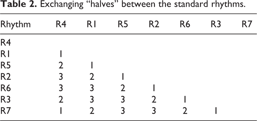
In addition, there have been proposals about how the different rotations relate to each other. In other words, how might the distances between them be measured? A circular representation of how the rhythms are related to one another is derived by a process called exchanging “halves” (Agawu, 2006). Each rhythm can be viewed as two approximate “halves”—or two sub-patterns, as mentioned earlier. One half consists of two 2s and a 1, making a total duration of 5, and the other half consists of three 2s and a 1, making a total duration of 7 (see Table 1). By dividing each rhythm into 5 + 7 or 7 + 5 and then exchanging the two “halves,” the seven rhythms can be arranged in the circular order R4, R1, R5, R2, R6, R3, R7. Figure 4 shows this arrangement with the “halves” (5 and 7) marked in square brackets and the exchanges marked by dotted lines. For example, when R1 is divided into 5 + 7, exchanging the two “halves” resulted in R4; when R1 is divided into 7 + 5, exchanging the two “halves” resulted in R5. Table 2 shows distances between the seven rhythms in terms of the number of exchanges needed between “halves.”
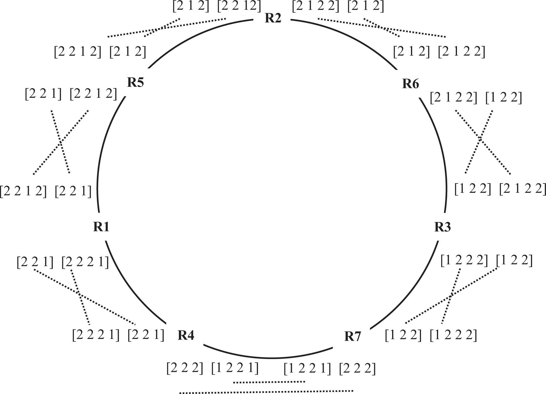
Exchanging “halves” for the standard rhythms. The seven rhythms are arranged in the circular order of R4, R1, R5, R2, R6, R3, R7. The square brackets arrange the structure of each rotation into two types of approximate “halves” (5 + 7 and 7 + 5). The dotted lines mark the exchanges between “halves” to transform one rhythm into a neighboring rhythm.
Exchanging “halves” between the standard rhythms.
Swap distance is another possible measure of perceptual distances between rhythms (Toussaint, 2013). It is the minimum number of swaps between adjacent pulse units necessary to transform one rhythm into another. Swap distance only applies to rhythms with the same number of events. Table 3(a) shows the seven rhythms in the order of R4, R1, R5, R2, R6, R3, R7, indicating each event by its clock position (1 = event, 0 = no event). Swapped positions are highlighted. For example, R4 can be transformed to R1 by swapping clock positions 5 and 6, making the swap distance 1. In turn, R1 can be transformed to R5 by swapping clock positions 10 and 11, making the swap distance 1. Accordingly, the swap distance between R4 and R5 is 2 (1 + 1). In other words, R4 can be transformed to R5 by swapping both clock positions 5 and 6, and clock positions 10 and 11. Table 3(b) shows the swap distance between every two rhythms. These two distance measures order the rhythms the same except that exchanging “halves” is a circular representation and swap distance is a linear representation with R4 and R7 farthest apart.
Standard rhythms and diatonic modes arranged according to swap distance.
(a) The swapping process

(b) Swap distance

Objectives of the Study
Experiment 1 was designed to explore the perceptual organization of the standard pattern; in particular, hierarchies of accents in the rhythms. Before describing the specifics of the method, it may be useful to emphasize the difference between rhythm and meter. As reviewed by Vuust and Witek (2014), rhythm refers to the pattern of discrete durations and is considered to depend on processes of perceptual grouping. Time is organized sequentially, and the perceptual organization depends on the pattern of temporal intervals. In contrast, meter contains a regular pulse or tactus, which is hierarchically differentiated into relatively strong and weak accents that recur with periodic regularity. Rhythmic events are perceived, at least in part, as accented according to the underlying metrical hierarchy. Rhythmic and metric accents often align but, according to London (2004), when rhythmic accent is not cued by duration or dynamics, the accents are often determined by the meter, a top-down process. This orientation seems to be generally accepted in research on metrical hierarchies, which is extensive (e.g., Ladinig, Honing, Haden, & Winkler, 2009; Large & Kolen, 1994).
However, an alternative process of bottom-up abstraction should also be considered. Listeners may impose a perceptual hierarchy on rhythms where some events naturally accrue perceptual accents independently of an underlying meter. It is thought that perceptual grouping is important for perceiving meter. So, for example, the first and last elements of a group may be heard as accented, as might longer tones or tones that precede gaps, or the first of a series of similar elements (Garner, 1974). Rhythmic events may also be accented by other factors, such as pitch contour, harmonic changes, and melodic parallelism (Lerdahl & Jackendoff, 1983). Thus, meter might not be the only factor governing rhythmic hierarchies and, moreover, there is no fixed relationship between grouping and metrical accent (Cooper & Meyer, 1960; Krumhansl, 2000; Lerdahl & Jackendoff, 1983). Although theories exist regarding rhythmic accents independently of meter, there is relatively little empirical evidence.
In order to probe specific temporal positions in the standard pattern, we dynamically accented one of the events in each rhythm by playing it louder than the other events in the rhythm. This is called the probe accent. The listener’s task was to rate how well the probe accent fit into the rhythm. We did this for each of the first seven events in each rhythm. This method was patterned after the probe tone method used to measure tonal hierarchies. In tonal music, one or more pitches are described as stable reference points, with other tones heard in relation to them. The tonic is generally considered the most important or stable tone in major and minor scales; other tones are heard as more or less related to it, creating a hierarchy (Krumhansl, 1990).
By analogy, certain time points in rhythms may be heard as stable reference points, with other time points heard in relation to them. For example, an up-beat in Western music is heard in relation to the beat that follows it (e.g., Lerdahl & Jackendoff, 1983). The assumption behind the probe accent method was that if a structurally stable or relatively strong event is dynamically accented, listeners will judge that the accent fits well into the rhythm. That is, if an event would usually be heard as accented perceptually, then actually accenting it would seem natural. However, if an event is heard that is usually perceived as weak, an accent on it would be judged as not fitting well. The resulting data will be considered in light of the various proposals summarized above for how events within the rhythms are organized and how they are related to one another.
We wanted to clearly distinguish between the seven rotations of the standard pattern. For that reason, we did not present the rhythms in a cyclical fashion, which would have deemphasized the starting point. In a performance context, the rhythms are repeated cyclically, and it is unclear how salient the starting points are perceptually, that is, whether the seven rotations are distinguished from one another. It is possible, for example, that they would be distinguished because of accents added by other instruments playing in the ensemble. In the experiment, each cycle was played twice in succession separated by a gap. The first presentation was intended to help the listener orient to the rhythm and locate the position of the accent, so that they could focus on it during the second presentation while they made their response.
Method
Participants
Forty-five students at Cornell University (7 males and 38 females, age 18–40 years) participated in Experiment 1 for course credit or USD 5 cash. Using repeated measures with a medium effect size of f = .25, α = .05, and a high power of .98, we have the estimated total sample size of 44. On average, participants had played music for 12.79 years (including music lessons; summed over all instruments and voice; range, 1–31 years; one person had no musical training). The study was approved by the university’s Institutional Review Board.
Apparatus and Stimulus Materials
We constructed seven rhythms based on the standard pattern by shifting the starting tone duration (see Figure 2(a) and Table 1). All rhythms consisted of eight monotonic tones on C4, forming seven time intervals. On each trial, only one temporal position was accented by increasing its loudness by 6.5 decibels, forming the probe accent. The probe accent was on one of the first seven events in each rhythm. All rhythms were at the tempo of 140 quarter notes per minute (i.e., each quarter note lasts approximately 429 ms) and were sounded in piano timbre. The tempo of 140 quarter notes per minute, or 93.3 dotted quarter notes per minute, is within the 80–170 beats per minute range, which is considered as the “tactus level” (Lerdahl & Jackendoff, 1983). On each trial, the rhythm was played twice, separated by a silence that lasted 3 quarter notes (each trial lasted approximately 7.29 s). Also constructed were seven unaccented rhythms, called the neutral rhythms, which were identical to the accented rhythms except that all the tones were played at the same loudness level. All stimuli used in Experiment 1 are provided online (http://music.psych.cornell.edu/M_and_S_Isomorphism/Experiment1/).
Procedure
Participants rated how well the probe accent fit into the rhythm by moving a slider on a continuous scale ranging from extremely bad fit (left end) to extremely good fit (right end). They began with four practice trials. Next, they listened to each of the 49 probe accent trials, which were blocked by rhythm type (i.e., R1, R2, etc.). Each block began with the neutral rhythm in order to familiarize the listener with the rhythm in the block. The seven blocks were presented in a randomized order within which the seven probe accent trials were played in randomized order. Following all the probe accent trials, participants listened to each of the seven neutral (unaccented) rhythms in a randomized order and rated them on two scales: 1) how familiar the rhythm was prior to the experiment and 2) how well-formed the rhythm seemed, in other words, whether or not the rhythm formed a good pattern. At the end of the study, participants filled out a demographics questionnaire. The experiment lasted approximately 30 minutes.
Results
All continuous rating scales were coded from −100 to 100. A mixed model linear regression on the familiarity ratings of the seven neutral (unaccented) rhythms was conducted with participants as a random variable. We found significant differences between rhythms (F(6, 264) = 4.98, p < .0001, ΔBIC = model BIC – participant BIC = 5.66). A post-hoc test (Tukey HSD) showed that R4 was rated as the most familiar and R7 was rated as the least familiar; the remaining rhythms were not statistically different from each other. As can be seen in Table 1, R4 is the rhythm that starts with the longest run of long durations. In contrast, R7 starts with a short duration followed by only two long durations before the next short duration. The same ordering was found for the well-formedness ratings (F(6, 264) = 7.04, p < .0001, ΔBIC = −5.49), which significantly related to familiarity (F(1, 269) = 111.18, p < .0001, ΔBIC = −111.69).
Hierarchies Within the Rhythms
Figure 5 shows the probe accent ratings for each of the seven rhythms plotted according to serial position and labeled by clock position so that durations can be determined by the values on the x-axis. For all the rhythms, there are peaks at the first and third serial positions. There is a third peak for all the rhythms except R7, which was judged the least familiar and least well-formed. For R1, R2, R4, and R5, the third peak is at serial position 5. For R3 and R6, the peak is at serial position 6. These two are the only rhythms in which the event in serial position 6 is preceded by a short event in serial position 5, suggesting the accent is perceived as more stable on the long event following the short event.

Probe accent ratings of each rhythm (y-axis; full range [-100, 100]) in the standard pattern labelled by clock position (x-axis). The serial positions line up vertically across rhythms. Error bars indicate 95% confidence interval.
The general pattern in the probe accent judgments of three peaks across the rhythms suggests that they perceptually divide into three groups with the accent being more stable on the first event in each group. Thus, the preferred grouping appears to be 2 + 2 + 3 events, except when the fifth event is a short tone followed by a long tone, then the preferred grouping appears to be 2 + 3 + 2. In the statistical analysis, serial position and rhythm were coded as categorical variables, and participants as a random effect. A mixed-model linear regression on the probe accent data with serial position as the factor was significant (F(6, 2149) = 23.26, p < .0001, ΔBIC = −89.55). A post-hoc Tukey HSD test showed the highest ratings overall were for accents in serial positions 1, 3, 5, but note the shift to serial position 6 for R3 and R6. Rhythm was not significant.
Table 4 lists the remaining features that were tested, and the second column details their numerical coding. Tone duration codes whether the accented tone was short (eighth note) or long (quarter note). Metrical hierarchies were coded by assigning the largest number (4) to the strongest metrical level and the smallest number (1) to the weakest metrical level, with intermediate levels (3 and 2) in between. For example, Figure 3 shows the coding of the 3/2 metrical hierarchy (4 1 2 1 3 1 2 1 3 1 2 1) as the numbers in parentheses. These were then assigned according to when events occurred in the rhythms. For R1, for example, the seven events in the rhythm were thus coded 4 2 3 1 1 1 1. Implicitly, this assumes that the first event is the downbeat. An alternative would be to substitute 3 for 4 in each code, for example, 3 1 2 1 3 1 2 1 3 1 2 1 for 3/2. Codes for the syncopation-shifted metrical hierarchy were derived from the codes for metrical hierarchy as described above. The bolded temporal positions in Table 4 indicate the positions that would inherit the larger weight from the following temporal position when no event occurs there (as seen in Figure 3).
Coding and results from the mixed-model linear regression analysis on features of the standard pattern.

Note. ΔBIC = model BIC – participant BIC.
We conducted a separate mixed-model linear regression analysis of the probe accent ratings with each coded feature, with the results shown in the third and the fourth columns of Table 4. As can be seen, syncopation-shifted 3/2 metrical hierarchy was by far the strongest feature, and the only nonsignificant feature was tone duration. Adding the other five metrical hierarchies to the model with only syncopation-shifted 3/2 metrical hierarchy did not result in a better fit (ΔBIC = 18.63). The alternative coding not assuming the first event was the downbeat resulted in a weaker effect. R3 and R7 are the two rhythms that start short-long which might suggest an upbeat-downbeat pattern. However, note that for these rhythms, ratings of the accent on the first event is considerably higher than the second event.
To further examine the generality of the syncopation-shifted 3/2 metrical hierarchy across the rhythms, it was tested for each rhythm separately. The statistical result was significant for all seven rhythms individually (R1: F(1, 269) = 29.15, p < .0001, ΔBIC = −22.03; R2: F(1, 267) = 11.41, p < .001, ΔBIC = −6.24; R3: F(1, 266) = 20.62, p < .0001, ΔBIC = −14.10; R4: F(1, 269) = 44.31, p < .0001, ΔBIC = −35.42; R5: F(1, 269) = 20.56, p < .0001, ΔBIC = −14.13; R6: F(1, 269) = 9.19, p < .01, ΔBIC = −3.32; R7: F(1, 269) = 8.46, p < .01, ΔBIC = −2.61). However, the syncopation-shifted 3/2 metrical hierarchy tended to fit the data best for those rhythms (R1, R4, R5) in which no syncopation shift had occurred in the first half of the rhythm. In these cases, events had occurred on strong metrical positions 0 and 4. The syncopation-shifted 3/2 metrical hierarchy fits the data less well for those rhythms (R2, R3, R6, R7) in which a syncopation shift occurred at clock position 3. This suggests that a longer and more regular rhythmic context preceding the syncopation shift makes it more prominent.
Distances Between Rhythms
To quantify the perceived distances among the seven rhythms, we calculated city-block distance. The city-block distance between any two rhythms was calculated as the sum of the absolute difference in probe ratings at each corresponding serial position. For example, to calculate city-block distance between R1 and R2, we found the absolute difference of the ratings of accents on the first event in R1 and R2, repeated this for the accents on the other six events, and then summed the seven absolute values. This creates a matrix of distances between all possible pairs of rhythms, shown in Table 5.
City-block distance between the standard rhythms.
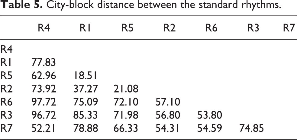
This matrix was then correlated with the two theoretical measures of distances between rhythms, which are exchanging “halves” (see Table 2) and swap distance (see Table 3(b)). Exchanging “halves” (r(19) = .49, R2 = .24, F(1, 19) = 5.85, p < .05) and swap distance (r(19) = .49, R2 = .24, F(1, 19) = 6.07, p < .05) accounted for an equal amount of the variation in city-block distances. Both measures order the rhythms as R4, R1, R5, R2, R6, R3, R7, but the first is a circular representation and the second is a linear representation. To examine this in more detail, the city-block distances were plotted against swap distance and the result was somewhat curvilinear. Supporting this, a polynomial regression to degree 2 provided a better account of the city-block distances (R2 = .33, F(2, 18) = 4.34, p < .05) than swap distance. Thus, R4 and R7 were closer than predicted by swap distance but not as close as in the circular representation of exchanging “halves.”
Discussion
The probe accent ratings for the seven rhythms showed two perceptual influences. The first related to how the events were organized into subgroups. The rhythms tended to subdivide into three subgroups that were of different durations. These subgroups could be understood in terms of a number of underlying perceptual principles that contributed to grouping. First, the relatively high ratings for accents in serial position 1 suggest that listeners find an accent on the first event to be rhythmically stable. This was true regardless of whether the first event was short or long. Secondly, the relatively high ratings on serial position 3 suggests listeners prefer groups of two. Previous research has found a general preference for duple grouping in isochronous sequences (Brochard, Abecasis, Potter, Ragot, & Drake, 2003; Martens & Benadon, 2017). These data suggest that the preference for duple grouping might extend also to non-isochronous rhythms. Alternatively, or in addition, this result might reflect a preference for alternating between contrasting levels of stress, perhaps analogously to speech. These two preferences provide evidence for Locke’s (1982) idea that both identifying the cycle and hearing the accents within that cycle are important cognitive principles for the standard rhythms.
There were two rhythms (R3 and R6) where the second sub-group contained three rather than two events and the more stable accent occurs on serial position 6 instead. These are both cases where a short event in serial position 5 precedes a long event in serial position 6. Thus, a preference for an accent on a long event following a short event can override the preference for groups of two. In addition, accents never received high ratings in serial position 7, the penultimate tone, with the stress likely accruing to the immediately following final tone. The subgroups of 2 + 2 + 3 and 2 + 3 + 2 together suggest a preference for balanced grouping, where each subgroup consists of a roughly equal number of events (Handel & Todd, 1981). Finally, the highest familiarity and well-formedness ratings of R4 suggest the preference for beginning a rhythmic sequence with the longest run of identical events (the same tone duration). This run principle is consistent with early evidence on the perceptual organization of temporal patterns (Handel, 1974; Preusser, Garner, & Gottwald, 1970).
The second perceptual influence apparent in the results is described by the syncopation-shifted 3/2 metrical hierarchy proposed by Temperley (1999, 2000). It modifies the metrical hierarchy for 3/2 to accommodate the effect of syncopation, which also provides evidence for Locke’s (1982) observation of shifting accents. When an event is not sounded at a time point that would normally be heard as metrically strong, its metrical weight transfers to the immediately preceding time point where an event is sounded. This theoretical proposal provided a much better account than any of the other metrical hierarchies that were tested. It also fits the data well across each of the seven rhythms individually. However, there was a slight tendency to fit the data better for rhythms in which the first syncopation shift occurred later in the sequence. These rhythms began with a longer, more regular beginning, which may have contributed to the salience of the later syncopation shift. To sum up, the probe accent results showed hierarchies that depended on two types of influences: those following principles of grouping, and those following metrical principles modified to account for the effect of syncopation. Thus, as predicted by Locke (1982) and Pressing (1983), these perceptual principles appear to work together despite the complex relationship between grouping and meter.
Finally, the probe accent data also tested two theoretical measures of distances between rhythms: exchanging “halves” and swap distance. Both order the rhythms the same way, except that exchanging “halves” is a circular model and swap distance is a linear model. The distance measure derived from the empirical data was a measure of the similarity of the probe accent ratings for all pairs of rhythms. Two rhythms were considered close if the ratings of the accents in the corresponding seven serial positions were similar. These distances derived from the data ordered the rhythms in the same way as both exchanging “halves” and swap distance, with a curvilinear component that suggested a model lying somewhat between the circular and linear models.
One question that might arise concerns the extent to which the probe accent results of this experiment would extend to the situation in which the rhythm is played in a repetitive cycle as it generally occurs in music. This would tend to deemphasize the starting point, and consequently the listener’s perception would be expected to be governed less by principles associated with the starting point, such as serial position and the syncopation-shifted 3/2 metrical hierarchy. However, there may still be influences of principles that do not depend on the starting point; in particular, preferring accents on a long event following a short event, and a preference for subgroups of approximately equal size, especially subgroups of two.
Experiment 2
Pressing (1983) noted that the diatonic scale pattern, which is the most prominent scale in Western tonal music, is isomorphic to the standard rhythmic pattern in Experiment 1. Scales with the diatonic pattern can be characterized by two common structural properties (Agmon, 1989): their scale steps (i.e., 12 for the diatonic pattern) and the diatonic intervals in the cycle (i.e., 7). The scale in the form of C D E F G A B is referred to as the parent scale (Rechberger, 2008), and the other six related scales in the diatonic family are traditionally viewed as modes. The diatonic pattern is rotational, such that the seven starting points generate seven unique patterns (see the last three columns in Table 1). Figure 2(b) illustrates the same scales in terms of tone identity (C, Db, D, etc.).
According to Powers (2001), mode applies to three separate stages of Western music: Gregorian chant, Renaissance polyphony, and tonal harmonic music of the 17th century to the 19th century. As a theoretical concept, mode was originally concerned with classifying scales according to such elements as the final scale degree, and the first and the fourth scale degrees. In the 20th century, in connection with music of other cultures, the term mode has broadened to include melodic and motivic features. In the present context, we use mode in the first sense, as a scale beginning and ending on a certain tone and containing a specific pattern of intervals between tones.
In this section, we will briefly describe three types of features that will be considered in analyzing the probe tone data. We call the first type basic features, and these are shown in Table 6. The first basic feature is the interval size between each tone and the next tone as measured in semitones. In the experiment, we used both ascending and descending scales. For example, for the ascending scale C D E F G A B C, C was coded as 2, D was coded as 2, E was coded as 1, and so on; for the descending scale C B A G F E D C, C was coded as 1, D was coded as 2, E was coded as 2, and so on. Three other features are coded with respect to the tone C. The first is primacy, which codes how early in the context sequence the probe tone occurred after C. The second is distance from C on the chroma circle; the third is distance from C on the circle of fifths. Krumhansl (1990) reported an experiment in which a major or minor context was followed by two tones and listeners rated how well the second followed the first. The judgments were influenced by the distance between the tones on the chroma circle and the circle of fifths, which suggested including these variables in the analyses.
Coding and results from the mixed-model linear regression analysis on basic features of the diatonic pattern.

Note. ΔBIC = model BIC – participant BIC.
The second type is called tonal features, the first of which is consonance between the probe tone and the tone C. Krumhansl (1990, Table 3.1) lists six different consonance measures that were obtained perceptually or computationally. Kameoka and Kuriyagawa (1969) plotted dissonance values for pairs of tones using the first six harmonics based on simple-ratio tuning; Malmberg Data (1918) measured listeners’ preference of two-tone intervals; Malmberg Ranks (1918) combined perceptual data and mathematical calculation on 10 different treatments (i.e., various instrumental timbres and adjectives that describe consonance) on the topic from the 12th to the 20th century; Helmholtz’s (1885/1954) equal-tempered and simple ratio measures were based on calculations from equal-tempered tuning and simple-ratio tuning, respectively; Hutchinson and Knopoff (1978) computed the total dissonance of pairs of tones using the first 10 harmonics with relative amplitudes of 1, 1/2, 1/3, and so on, based on equal-tempered tuning. Three more recent measures were also considered. McDermott, Lehr, and Oxenham (2010) obtained pleasantness ratings of two-tone chords in four different timbres, out of which, the synthetic tone in their Figure 1a is most similar to the stimuli used in the current study. Stolzenburg (2015, see Table 3) computed smoothed relative periodicity of dyads. Bowling, Purves, and Gill (2018) obtained dyad ratings of consonance, defined as pleasantness or attractiveness, rank ordered in their Figure 1a.
Other tonal features are also included. Large (2010) proposed the oscillatory neurodynamic model that predicted human judgments of perceived stability of tones in C major and C minor modes. We calculated the values for each tone in the diatonic pattern using the formula in Large, Kim, Flaig, Bharucha, and Krumhansl (2016). Gill and Purves (2009) computed the mean percentage similarity of tone combinations to the harmonic series, which is called harmonicity; the ordering of intervals corresponds quite well with the measures of consonance just described. The final three measures come from the study by Krumhansl and Kessler (1982). We used the C major profile because it is exactly M1 (see Table 1 for description of the modes used), and we used the C minor profile due to the large number of flat tones occurring in Experiment 2, and it is one of the scales, M6. We also used the major profile for each mode corresponding to the number of accidentals (C major for M1, Bb major for M2, Ab major for M3, G major for M4, F major for M5, Eb major for M6, and Db major for M7).
The third type is modal features. Figure 3 of Huron and Veltman (2006) shows the frequency of occurrence for each pitch class in church modes in a random sample of 98 Gregorian chants. The samples were larger for some modes than others, so we converted the values to percentages. Out of the eight mode profiles, the Dorian and the Hypomixolydian modes can both correspond to M2, so we considered both scenarios.
As with the rhythms, swap distance can be used to measure the distances between modes. This linear representation of mode distances is illustrated in Table 3(a); the resulting distance values are shown in Table 3(b). The ordering corresponds to the number of sharps and flats. It might be of interest that swap distance is related to a way of differentiating between modes (Curtis, 1992; Power, 2001). Table 7(a) shows the three types of species of the 4th (3 intervals covering a span of a fourth). Table 7(b) shows the four types of species of the 5th (4 intervals covering a span of a fifth). Table 7(c) shows how each mode can be expressed as one species of the 4th and one species of the 5th. The ordering in swap distance can be derived by identifying the overlapping species, highlighted in table.
Species of the 4th and species of the 5th in the diatonic pattern.
(a) Types of species of the 4th

Note. T: whole tone; S: semitone.
(b) Types of species of the 5th

Note. T: whole tone; S: semitone.
(c) Possible combinations for each mode
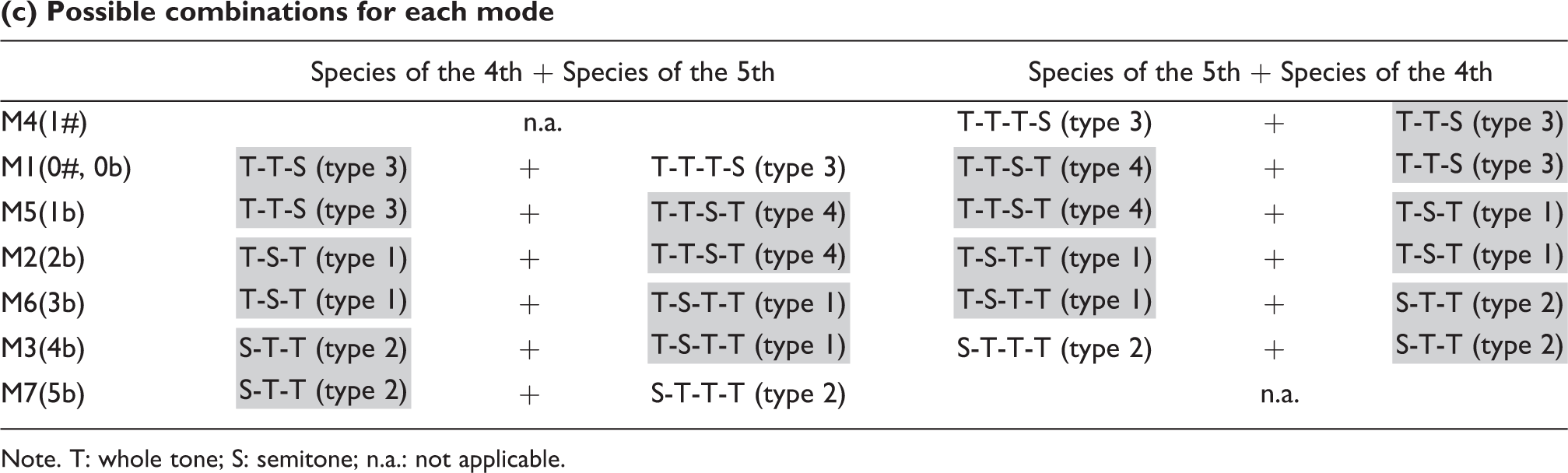
Note. T: whole tone; S: semitone; n.a.: not applicable.
Finally, modes are often differentiated based on modal ethos, or emotion. Powers (2001, Table 10) summarized Zarlino’s modal ethos of the twelve Glarean’s modes, which correspond as follows: M1 = 11, M2 = 1, M3 = 3, M4 = 5, M5 = 7, M6 = 9, M7 = 4. In the order M4, M1, M5, M2, M6, M3, and M7, modes toward one extreme have positive ethos (M4 = “joyous, modest and pleasing”; M1 = “suitable for dances, lascivious”) and modes toward the other extreme have negative ethos (M3 = “somewhat hard, moves one to weeping”; M7 = “lamenting sad, supplicant lamentation”). An interesting exception is that M6 is relatively positive (“cheerful, sweet, soft and sonorous”), placing it nearer to M1, its parallel major. Experimentally, Temperley and Tan (2013) showed that the emotion connotation of modes in the diatonic pattern ranged from the happiest to the saddest in the same order (M7 was not tested), except M1 was judged happiest, likely due to familiarity. Both the theoretical modal ethos and the empirical emotion connotations suggest that the “sharpness” of a mode correlated with perceived happiness.
Objectives of the Study
Experiment 2 was designed to determine the tonal hierarchies of the modes using the probe tone technique (Krumhansl & Shepard, 1979), in which a probe tone is played after the mode context. The mode context is played in either an ascending or descending form with different pitch ranges so that the probe tones are always in the same range. Listeners rated how well the probe tone fit into the context using the seven pitches in each mode. Using the probe tone method, the current study obtains a profile of perceptual stability for all pitches in each of the seven modes. These data are analyzed for the effects of the features described above: basic, tonal, and modal. The data are also used to test the distance representation.
Method
Participants
Forty-five students at Cornell University (6 males and 39 females, age 18–40 years; 31 also participated in Experiment 1) participated in Experiment 2 for course credit or USD 5 cash. We used the same power analysis as in Experiment 1 to estimate the sample size for Experiment 2. On average, they had played music for 14.0 years (including music lessons; summed over all instruments and voice; range, 1–29; three had absolute pitch, and one had no musical training). The study was approved by the university’s Institutional Review Board.
Apparatus and Stimulus Materials
We constructed seven modes based on the major diatonic mode by shifting the starting pitch interval (see Figure 2(b) and Table 1). All modes consisted of eight isochronous tones, each lasted for a quarter note, forming seven pitch intervals. Each mode was constructed in both ascending and descending forms, beginning and ending on C. The range of the ascending sequence was C3 to C4, and the range of the descending sequence was C6 to C5 (as in Krumhansl & Shepard, 1979). The seven modes were followed by a probe tone in the range that extends from the preceding sequence. The probe tone was played in the range of Db4 to C5 for the ascending mode and C4 to B4 for the descending mode. Only the seven tones in each mode were used as probe tones. The pause of silence in between the mode and the probe tone lasted for two quarter notes. All mode contexts were at the tempo of 140 quarter-note per minute (each quarter note lasts approximately 429 ms; each trial lasted approximately 4.71 s) and was sounded in piano timbre. Also constructed were seven modes without a probe tone after the context, called the neutral modes. All stimuli used in Experiment 2 are provided online (http://music.psych.cornell.edu/M_and_S_Isomorphism/Experiment2/).
Procedure
Participants rated how well the probe tone fit into the scale by moving a slider on a continuous scale ranging from extremely bad fit (left end) to extremely good fit (right end). They began with four practice trials. Next, they listened to each of the 98 probe tone trials (49 ascending and 49 descending), which were blocked by mode type (i.e., M1, M2, etc.); the ascending and descending modes were intermixed. The 7 blocks were presented in a randomized order. Each block began with the neutral mode played twice, once ascending and once descending, to familiarize the listener with the mode to be presented in the block. This was followed by 14 probe tone trials of the same mode played in randomized order. Following the probe tone ratings, participants listened to each of the seven neutral modes (without the probe tone) in ascending form, in the range of C4 to C5, in a randomized order and rated them on two scales: 1) how familiar the scale was prior to the experiment, and 2) how well-formed the scale seemed, in other words, whether or not the scale formed a good pattern. At the end of the study, they filled out a demographics questionnaire. The experiment lasted approximately 30 minutes.
Results
All continuous rating scales were coded in the same way as in Experiment 1. A mixed-model regression analysis found some modes were more familiar than others (F(6, 263) = 16.67, p < .0001, ΔBIC = −52.03). A post-hoc test (Tukey HSD) showed that M1, the major diatonic scale, was rated as the most familiar, M7 was rated as the least familiar; the others were not different statistically. The well-formedness ratings were similar, except that M2 was not statistically different from M7 (F(6, 264) = 22.05, p < .0001, ΔBIC = −75.09). The well-formedness ratings were significantly related to familiarity (F(1, 268) = 149.93, p < .0001, ΔBIC = −113.00).
Hierarchy Within a Mode
Figure 6 shows the probe tone ratings of each of the seven modes plotted according to the tone identity of the probe tone and whether the context was ascending or descending. In the mixed-model linear regression with tone identity as the fixed effect and participants as the random effect, tone identity was highly significant (F(12, 4352) = 63.35, p < .0001, ΔBIC = −601.83). A post-hoc Tukey HSD test showed C was higher than all other tones; it was followed by G. Then the test identified a group containing Db, D, F, Ab, Bb, and B which were not significantly different from each other. With the exception of Ab, these tones are either proximate to C (Db, D, Bb, and B) or close to it on the circle of fifths and also consonant with it (F). The tritone from C, F#/Gb, always received the lowest ratings when it was present (M4 and M7). A similar analysis using mode as the fixed effect showed no effect.

Probe tone ratings of each mode (y-axis; full range [−100, 100]) in the diatonic pattern labelled by tone identity (x-axis), with ascending on the left and descending on the right. The serial positions line up vertically across modes. Error bars indicate 95% confidence interval.
Basic Features
We first conducted a separate mixed-model linear regression analysis on each basic feature shown in Table 6. As can be seen, all these variables were statistically significant. Primacy was a very strong predictor of the probe tone ratings. That is, listeners highly rated probe tones that matched the chroma of tones sounded early in the context. In general, listeners perceived tones to be more stable when they were close to the C on the circle of fifths, and to a lesser extent, on the chroma circle, over those that were farther from the C. These results support the idea that the C, which was sounded first and last in the context, served as a reference point. Interval size had a relatively weak effect. When all the basic features were entered into one regression model, interval size was only marginally significant.
Consonance, Tonal, and Modal Features
All the consonance measures that were mentioned earlier under tonal features correlated significantly with the probe tone ratings (at p < .0001, ΔBIC range [−327.57, −44.72]) except for the values of McDermott et al. (2010) which had no value for the tone C. This suggested that the significant correlations for the other consonance measures might be largely driven by the high ratings of the tone C. When the C was removed from the statistical analysis, only two remained significant: the values from Kameoka and Kuriyagawa (1969, Figure 8) and Helmholtz Equal-Temperament (1885/1954, p. 332). Other features were also correlated (at p < .0001, ΔBIC range [−457.41, −53.23]) with the probe tone data: the prediction of the neurodynamic model (Large, 2010), harmonicity (Gill & Purves, 2009), the C major and C minor probe tone profiles (Krumhansl & Kessler, 1982), and the major profiles of the keys corresponding to the number of accidentals. When C was excluded from the analysis, the predictions of the neurodynamic model were no longer significant, but the other predictors remained significant (at p < .01, ΔBIC range [−46.11, .01]). Finally, the distribution of tones computed as percentages in Huron and Veltman’s (2006) Gregorian chant corpus did not significantly correlate with the probe tone data assuming either M2 = Dorian or M2 = Hypomixolydian.
Distances Between Modes
To quantify the perceived distances between the seven modes, we calculated city-block distance in the same way as for the seven rhythms in Experiment 1. C received the highest rating for all the modes, so we considered it to be the first scale degree for each mode, with the remaining tones considered scale degrees 2, 3, and so on. In the context of modes, city-block distance is the sum of the absolute difference in probe tone ratings for each scale degree. This creates a matrix of distances between all possible pairs of modes (see Table 8). This matrix of city-block distances correlated significantly with swap distance (r(19) = .85, R2 = .72, F(1, 19) = 47.69, p < .0001). This result suggests that the distances between modes, as measured by the similarity of their probe tone ratings, can be quite well accounted for by swap distance, which corresponds to the number of sharps and flats.
City-block distance between the diatonic modes.

Discussion
The probe tone ratings for the seven modes showed a number of underlying perceptual influences. The first was how early the probe tone was sounded in the context, the second was proximity to C on the chroma circle, and the third was proximity to C on the circle of fifths. On balance, consonance had a relatively weak effect on the probe tone ratings, but stronger effects were found for harmonicity (Gill & Purves, 2009) and tonal hierarchies (Krumhansl & Kessler, 1982). These results suggest listeners were basing their judgments in part by reference to tonal hierarchies in the more familiar major and minor keys. Lastly, we found no significant relationship between the probe tone ratings and the distribution of tones in Huron and Veltman’s (2006) corpus study of Gregorian chants.
The swap distance measure predicted the perceptual distances between modes, which also orders the modes according to the number of accidentals (and as on the circle of fifths). The order was also supported by the ordering as on the circle of fifths based on the probe tone profiles for keys. The order generally fits with the ordering of modes in terms of positive to negative affect (Powers, 2001; Temperley & Tan, 2013).
One question that might arise concerns the extent to which the probe tone ratings for the seven diatonic modes played in scalar form would extend to modal music in which the tones are not generally played in scalar form. The results of Krumhansl and Shepard (1979), which used ascending and descending scales, generally agree with probe tone results using other contexts such as chords and melodies (Krumhansl & Kessler, 1982; Oram & Cuddy, 1995; Schmuckler, 1989). Given this, some of the principles supported by the present probe tone ratings might extend to non-scalar modal music, such as chroma and circle of fifth distance from the final of mode.
Experiment 3
A basic question in music cognition is how the dimensions of pitch and time combine. The literature has found two different kinds of relationships (as summarized in Krumhansl, 2000; Prince 2011; Prince & Schmuckler, 2014). One is that pitch and time are two separable dimensions, where changes in one dimension do not affect the perception of the other dimension. The other is that pitch and time interact perceptually, where changes in one dimension affect the perception of the other dimension. The current experiment is concerned with the effect of the alignment between pitch patterns and rhythmic patterns on the perception of the combined pattern; specifically, whether the rhythm is heard as fitting well with the mode. We will briefly review studies that have focused on combined pitch–time patterns in particular and explored the various factors that seem to promote one type of processing over the other.
A number of studies have supported the idea that pitch and time are two separable dimensions. An early study found pitch and time made independent contributions to melodic similarity judgments, with trade-offs between rhythmic and pitch factors (Monahan & Carterette, 1985). Palmer and Krumhansl (1987a, 1987b) investigated how pitch and time influence judgments of phrase endings by shifting the melody relative to the rhythm. The judgments were consistent with an additive model of the final tone’s position in tonal and metrical hierarchies. Prince and Pfordresher (2012) used combinations of rhythmic and pitch patterns that varied in complexity by manipulating the number of distinct durations and pitches. The numbers independently influenced complexity judgments. Prince (2014) investigated how surface and structural properties of pitch and time affect the perceived similarity of melodies. When manipulated independently, they made independent contributions to similarity judgments.
Other studies, however, demonstrate interactions between pitch and time. Deutsch (1980) found more accurate dictation when the groups in the pitch pattern coincided with the groups in the temporal pattern. Jones, Summerell, and Marshburn (1987) demonstrated better recognition of melodies when played in the original rhythms than in a novel rhythm. Boltz (1995) presented a set of folk tunes in which tones were prolonged either at phrase endings or somewhere else within the phrase. For the latter, duration judgments were less accurate. Boltz (1998) found similar effects for tempo judgments. Prince (2011) asked listeners to selectively attend to pitch (i.e., tonality), time (i.e., meter), or both, and judge melodic goodness. They were unable to ignore the unattended dimension; interactions were strong when attending to both dimensions. Prince and Loo (2017) found similar failures in selective attention in expectancy ratings. Prince and Pfordresher’s (2012) participants made more reproduction errors in one dimension when the other dimension was more complex.
Finally, a corpus study of compositions by Bach, Mozart, Beethoven, and Chopin showed that tonally stable pitch classes disproportionately fell on temporally stable positions (Prince & Schmuckler, 2014), that is, metrical and tonal hierarchies coincide. Similarly, corpus studies of bebop-styled jazz showed that improvisers emphasized the tonally prominent chords at metrically prominent temporal positions (Järvinen, 1995; Järvinen & Toiviainen, 2000). These findings suggest that the perceptual question concerning how pitch and time interact has significance for how these dimensions are combined in music.
Prince, Schmuckler, and Thompson (2009) and Prince (2011) summarized various factors that might explain these different results. One explanation concerns whether the information is processed early or late. One proposal has been that pitch and time are initially processed separately (e.g., pitch height and tempo) and are later integrated (e.g., melodic completion and similarity) (Hébert & Peretz, 1997; Peretz & Kolinsky, 1993). A second explanation is related to whether the task focuses on a local event or whether it focuses on a global property of a longer sequence. Experimental tasks that focus on a local event (e.g., a specific chord or rhythmic event) are likely processed independently whereas tasks that attend to a global property that spans across a larger time period (e.g., tension and relaxation within a sequence) require processing of integrated pitch and time information (e.g., Tillmann & Lebrun-Guillaud, 2006). A third explanation is the degree of perceived musical coherence of the musical context (Boltz, 1999). Pitch and temporal information tend to be processed in a unified way when a melodic sequence has high musical compatibility, where the pitch structure (e.g., phrase) and the temporal structure (e.g., rhythm) are consistent with each other (e.g., coincide). In contrast, dimensions in less coherent contexts (e.g., misaligned structures) might be processed separately.
Prince (2011) pointed to two other factors that might affect how pitch and time are processed. First, he distinguishes the differences between tasks that monitor relatively surface aspects of the music (e.g., contour or pattern of durations) and more abstract structures (e.g., tonal and metrical hierarchies). In the former case, the dimensions might be processed more independently than in the latter case. The second factor is the relative salience of the dimensions. If there is a tendency for one perceptual dimension to be more salient (i.e., pitch may be more prominent for Western listeners), it may dominate the other (i.e., time), resulting in an asymmetric interaction between pitch and time.
Objectives of the Study
Experiment 3 tested whether listeners perceive specific rhythmic patterns to fit well with specific pitch patterns, using the theoretically isomorphic standard pattern and diatonic patterns. Each rhythm was combined with each mode to create a total of 49 (7 × 7) combinations, and listeners judged how well the rhythm fit the scale. For brevity, we call these fit judgments. Two possible outcomes were tested: 1) that listeners will prefer the large pitch interval (ascending whole tone) to coincide with the long tone duration, an intervallic-level match, and 2) that they will prefer tonally stable tones, as measured in Experiment 2, to coincide with temporal positions where accents were preferred, as measured in Experiment 1, a hierarchical-level match.
Method
Subjects
Fifty students at Cornell University (15 males and 35 females, age 18–40 years) participated in Experiment 3 for course credit. We used the same power analysis as in Experiments 1 and 2 to estimate the sample size for Experiment 3. On average, participants had played music for 11.3 years (including music lessons; summed over all instruments and voice; range, 1–40; three had absolute pitch, and four had no musical training). The study was approved by the university’s Institutional Review Board.
Apparatus and Stimulus Materials
We constructed 49 rhythm–mode pairs by combining each of the seven rhythms in Experiment 1 with each of the seven ascending modes in Experiment 2 (Table 1). Descending modes were not used because the interval sizes would not then be isomorphic to the tone durations in the rhythms. The range of all sequences was C4 to C5. All stimuli were played in piano timbre at the tempo of 120 quarter notes per minute (each quarter note lasts approximately 500 ms; each trial lasts approximately 3.50 s). In addition, we used the seven unaccented rhythms and the seven modes without the probe tone as the neutral trials. All stimuli used in Experiment 3 are provided online (http://music.psych.cornell.edu/M_and_S_Isomorphism/Experiment3/).
Procedure
Participants rated how well the rhythm fit the scale by moving a slider on a continuous scale from extremely bad fit (left end) to extremely good fit (right end). They began with four practice trials. Next, they listened to and rated each of the 49 trials in randomized order. After completing a demographics questionnaire, they then repeated the same task one more time, with a different randomized order of trials. Following the fit judgment, participants completed another demographics questionnaire, and then listened to each of the 14 neutral trials (seven unaccented rhythms and seven modes without the probe tone) in a randomized order and rated them on two scales: 1) how familiar the rhythm or mode was prior to the experiment, and 2) how well-formed the rhythm or mode seemed, in other words, whether or not it formed a good pattern. The experiment lasted approximately 30 minutes.
Results
All continuous rating scales were coded in the same way as Experiments 1 and 2. Table 9 shows the average fit judgments across participants. A mixed-model regression analysis showed some rhythms were more familiar prior to the experiment than others (F(6, 293) = 4.25, p < .001, ΔBIC = 10.22); a post-hoc test (Tukey HSD) found R7 was rated as the least familiar, but the others were not statistically different. Some rhythms were also judged to be more well-formed than others (F(6, 294) = 4.20, p < .001, ΔBIC = 10.53); R4 was judged the most well-formed, and R7 the least well-formed; the others were not significantly different. The well-formedness ratings for rhythms were significantly related to familiarity (F(1, 298) = 106.89, p < .0001, ΔBIC = −104.91). Modes were also significantly different in terms of familiarity (F(6, 294) = 9.81, p < .0001, ΔBIC = −19.56); M1 was rated as the most familiar mode; the others were not different statistically. The same pattern held for well-formedness ratings which also differed significantly (F(6, 294) = 15.27 p < .0001, ΔBIC = −46.17). The well-formedness ratings for modes were significantly related to familiarity (F(1, 299) = 234.68, p < .0001, ΔBIC = −200.44). These results are similar to those in Experiments 1 and 2.
Average fit judgments of rhythm–mode combinations with the range [−100, 100].

Combinations of Rhythms and Modes
To test whether listeners perceive long tone durations to fit well with large pitch intervals, we coded the intervallic-level match in three ways. Table 10(a) shows the first coding. All isomorphic combinations (rhythms and modes that share the same structure in Table 1) were coded as 1 and all non-isomorphic combinations (rhythms and modes that do not share the same structure in Table 1) were coded as 0. Table 10(b) shows the second coding, which is based on the number of times that pitch interval and tone duration are matched. For example, as Table 1 shows, R1 and M4 are matched for the first two intervals (2 2 and T T, respectively) and the last three intervals (2 2 1 and T T S, respectively), making a total of five matches; R1–M4 was coded as 5. Table 10(c) shows the third coding. This was based on the number of matches prior to the first mismatch. For example, as Table 1 shows, R1 and M4 share the same structure (2 2 and T T, respectively) at the beginning of the sequence, and diverged at the third interval/duration (1 and T, respectively), making a total of two matches prior to the first mismatch; R1–M4 was coded as 2.
Coding of intervallic-level match of rhythm–mode combinations.
(a) The first type of coding based on exact match

Note. Matched pair = 1, mismatched pair = 0.
(b) The second type of coding based on total number of match

(c) The third type of coding based on number of match before the first mismatch

The correlation between the intervallic-level match and the fit judgments was not significant for the first two types of intervallic-level coding, but it was significant for the third type, the number of events that match before they diverge (F(1, 2400) = 13.01, p < .001, ΔBIC = −5.17). The high ratings for both probe accents and probe tones in the initial serial positions suggest a focus on early events in the sequence might be driving this effect. The correlation was no longer significant when these cases were excluded.
To test whether listeners perceive temporal positions where accents received high ratings, as measured in Experiment 1, to fit well with tonally stable tones, as measured in Experiment 2, we correlated the probe accent ratings from Experiment 1 with the probe tone ratings from Experiment 2 for each pair of rhythms and modes. We call these correlations the hierarchical-level match, shown in Table 11. For any particular pair, the correlation would be strong if the tonally strong events occurred when rhythmic accents received high ratings. The pair R1 and M4 (Figures 5 and 6) is a case in which accents received high ratings occur at tonally strong events. In contrast, R3 and M2 have dissimilar ratings, so their combination would place accents that received low ratings at tonally strong events. The hierarchical-level match had a strong effect on the fit judgments (F(1, 2400) = 195.16, p < .0001, ΔBIC = -179.83), shown in Figure 7. This means that the measure derived from Experiments 1 and 2 (the degree to which their hierarchies agreed) predicted well how the rhythm was judged to fit the scale.
Coding of the hierarchical-level match of rhythm–mode combinations by correlating the probe accent ratings from Experiment 1 and the probe tone ratings from Experiment 2.

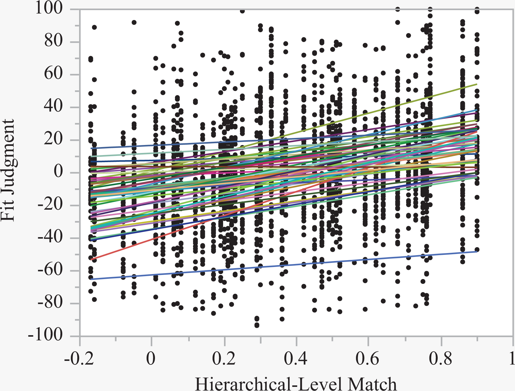
Correlation between the fit judgment from Experiment 3 (y-axis) and the hierarchical-level match that is derived from the probe accent ratings in Experiment 1 and the probe tone ratings in Experiments 2 (x-axis). The fit lines indicate the correlation trends for individual participants.
In addition, the fit judgments are accounted for by the familiarity of the rhythm (F(1, 2399) = 55.77, p < .0001, ΔBIC = −38.99), the familiarity of the mode (F(1, 2399) = 114.38, p < .0001, ΔBIC = −98.75), the well-formedness judgment of the rhythm (F(1, 2399) = 79.42, p < .0001, ΔBIC = −57.55), and the well-formedness judgment of the mode (F(1, 2399) = 162.97, p < .0001, ΔBIC = −146.33). The hierarchical-level match remained the strongest predictor of the fit judgments despite the effects of familiarity and well-formedness.
Discussion
When participants judged how well the rhythm fit the scale, higher ratings were given to combinations in which highly rated temporal accents (accents that were judged as fitting well with the rhythm contexts) took place at tonally strong events (tones that were judged as fitting well with the mode contexts). Thus, the results were well explained by an interaction at a hierarchical level between pitch and time. This was true even when familiarity and well-formedness of the rhythms and modes were taken into account. It should be noted that the task was asymmetrical in as much as it asked how well the rhythm fit the scale. So, the task specifically directed attention to the rhythm. Different results might be found for the opposite instruction focusing on the scale, or one that asks whether the rhythm and the scale fit together well.
This experiment provides another example of perceptual interactions between the pitch and time dimensions, rather than independent processing of the two dimensions. The result is in accord with explanations for the divergent findings in the literature (Prince, 2011; Prince, Schmuckler, & Thompson, 2009). The task of judging how well the rhythm fits the mode would rely on late processes because it focuses on the relationship between the two patterns, requiring the integration of the two dimensions. The task also emphasizes global processing, as the entire rhythmic sequence is to be compared with the entire mode. In addition, the two dimensions are matched in complexity. Given this, the two dimensions would likely be fairly well matched in salience. All these factors help understand why the results in the current experiment depended on the interaction on a hierarchical level.
General Discussion
In exploring pitch–time interaction, three experiments focused on two special cases of rhythmic and scale patterns, the standard rhythmic pattern and the diatonic scale pattern. Building on the substantial music theory interest on the intervallic parallels and matched complexity between the two patterns, we showed how pitch and time perceptually interact. The interaction is governed by a number of cognitive principles underlying the pitch and time dimensions. Some of these principles are shared, as suggested by Pressing (1983); others are distinct from each other, as argued by London (2002).
We turn first to the pitch–time interaction. When the modes were paired with the rhythms, listeners judged combinations in which accented events at rhythmically stable positions to fit well with tonally stable tones. Listeners did not prefer combinations in which events with longer durations took place at larger pitch intervals. Thus, fit judgments depended on the hierarchical-level match, not the intervallic-level match. That pitch and time interact in this way is consistent with a number of proposals about what task and stimulus characteristics favor perceptual interactions between dimensions rather than independent processing: late processing, global judgments, coherent patterns, abstract rather than surface properties, and balanced salience of the dimensions.
Support for the underlying cognitive principles is present at different levels: hierarchies within the rhythms and modes, familiarity and well-formedness, and distances between the rhythms and between the modes. At the level within the rhythms and the modes, different cognitive principles apply to pitch and time. Listeners tended to break the standard rhythmic pattern into three subgroups, suggesting a preference for duple grouping. Accents were perceived as rhythmically stable on the first event and on a long event following a short event, but not on the penultimate tone. In addition, the syncopation-shifted 3/2 metrical hierarchy proposed by Temperley (1999, 2000) had a consistent perceptual influence on the seven rotations of the standard pattern, especially when it did not occur until the second half of the sequence after a strong metrical context had been formed. The coexisting principles of subgrouping and of the syncopation-shifted 3/2 metrical hierarchy provide evidence for multiple cognitive principles working together, that is, multistability (Pressing, 1983).
In contrast, the probe tone ratings for the modes were dominated by relationships relative to the tone C, which began and ended sequences in both the ascending and descending contexts. Probe tones close to the initial C in the context, or close to it on either the chroma circle or the circle of fifths, were generally rated more highly; these have been shown to contribute to judgments of inter-tone distance (Krumhansl, 1990). The probe tone ratings also resembled to some extent the tonal hierarchies of C major and C minor (Krumhansl & Kessler, 1982) and the major keys corresponding to the number of sharps and flats. These different cognitive principles found for rhythmic and tonal hierarchies support London’s (2002) view of non-isomorphisms between pitch and time.
However, at the level of familiarity and well-formedness, the rhythms and the modes were rated similarly. Mode 1 and Rhythm 4 were rated as the most familiar and well-formed. Mode 1 is the major scale, namely, the most prominent scale in Western music. Rhythm 4 starts with the longest run of long durations, establishing a stable and regular pattern at the onset, which is consistent with the run principle and is typical of Western rhythms. At the other extreme, Mode 7 and Rhythm 7 were rated as the least familiar and well-formed. Mode 7 has the greatest number of accidentals among the modes. Rhythm 7 violates the run principle by starting with a short duration followed by a short run of long durations, beginning with the most irregular pattern. In addition, the modes and rhythms were similar in that pitch interval or temporal interval had little or no influence on the probe ratings.
At the level of inter-rhythm and inter-mode distances, pitch and time also showed perceptual similarity. The perceptual distance measure derived from the probe data corresponded best with the swap distance measure for both rhythms and modes, which arranges the rhythms and the modes in this order: R4/M4, R1/M1, R5/M5, R2/M2, R6/M6, R3/M3, R7/M7. This ordering corresponds to the relative number of sharps and flats. It also follows the emotion connotations of the modes from happy to sad found by Temperley and Tan (2013), except that M1 was judged happiest, perhaps because of familiarity. Finally, swap distance, a computational model of rhythmic distance, was found to correspond to the arrangement of the diatonic modes based on the species of the 4th and the species of the 5th, coming from a very different theoretical tradition.
A similar isomorphism between time and pitch was found in a recent study of polyrhythms and pitch intervals (Razdan & Patel, 2016). They translated the frequency ratios of the intervals from minor second to octave (plus major, minor, augmented, and diminished chords) into polyrhythms. The ratings of the polyrhythms for pleasantness correlated strongly with pleasantness ratings for the corresponding pitch intervals.
Other theoretical properties might suggest experiments that reveal additional cognitive principles in the future. At least three other theoretical properties are shared by the standard and diatonic patterns. The first characteristic is maximally even set. The seven positions in each rhythm and the seven pitches in each mode both form a set that is the closest to being spread evenly around the circle (Clough & Douthett, 1991; Toussaint, 2013). In other words, the seven dark circles in Figure 1 cannot be more evenly distributed around the 12 clock positions. The second characteristic is that the standard and diatonic patterns are both asymmetrical. Each tone has a unique set of relations from every other tone (Browne, 1981; Rahn, 1996; Temperley, 2000). As a result, for the scales, the asymmetrical distribution of the semitones facilitates position-finding based on only two or three tones. The function of position-finding might also be applicable to the rhythms. The third characteristic is that the standard pattern is a deep rhythm (Toussaint, 2013) and the diatonic pattern is a deep scale (Gamer, 1967; Johnson, 2003; Toussaint, 2005). For a pattern to be deep, the distance between every pair of onsets or pitches has to occur a unique number of times. All three theoretical properties suggest there may be other perceptual isomorphisms between standard and diatonic patterns that might be tested in future empirical studies.
A fundamental question in cognitive science is how information from different sensory dimensions is integrated to form a coherent representation of the external world. Garner’s (1974, 1976) empirical studies of cross-dimensional relationships were informed by two questions. The first question is whether or not information in one dimension can be processed independently of the other dimension. The second question is whether or not information in one dimension can facilitate or interfere with the processing of the other dimension. The empirical studies uncovered different kinds of relationships between dimensions. For separable dimensions, processing of one dimension is unaffected by variation in another dimension. In contrast, for integral dimensions, the two dimensions cannot be processed independently from one another, and the perception of one dimension facilitates or interferes with perception of the other dimension. In vision, saturation affects the perception of hue, but variation in shape does not affect the perception of color (Burns & Shepp, 1988; Garner, 1976). In haptics, size, shape, orientation, and weight all interact with each other (Kappers & Tiest, 2015). This distinction between separable and integral dimensions has been studied using various approaches, such as similarity measurements, classification tasks, preference judgments, and discriminability between preferences (Garner, 1974, p. 118).
In this context, music is an interesting case in which two dimensions, pitch and time, are each highly structured. This allowed us to ask for the musical patterns studied, the standard rhythmic pattern and the diatonic scale pattern, whether these dimensions interact and, if so, whether the interactions are on one of two levels. The first level concerns whether the intervals in the two patterns coincide, an intervallic-level match. The second level is whether tonally strong events occur at points in the rhythms where accents are preferred, a hierarchical-level match. Judgments of how well the rhythm fits the scale demonstrated that these dimensions interact in an integral fashion and, moreover, that the interaction is on the hierarchical level. In addition, the results of the studies quantifying the tonal and rhythmic hierarchies uncovered some common underlying principles, but also found different principles influenced the perceived hierarchies in the two dimensions. Thus, the interaction between the dimensions does not simply result from common cognitive principles, but rather derives from unique cognitive principles functioning in concert with one another. Finally, using the probe accent and the probe tone ratings in conjunction with the fit judgments provided a more in-depth understanding of the holistic perception of pitch and time in music.
Footnotes
Contributorship
OXW and CLK researched literature and conceived and designed the study. CLK gained ethical approval, OXW recruited participants and conducted experimental sessions for data collection. Both authors were involved in data analysis and manuscript writing. OXW wrote the first draft; both authors reviewed and edited the manuscript and approved the final version.
Declaration of conflicting interests
The author(s) declared no potential conflicts of interest with respect to the research, authorship, and/or publication of this article.
Funding
The author(s) received no financial support for the research, authorship, and/or publication of this article.
Peer Review
Steffen Herff, École Polytechnique Fédérale de Lausanne (EPFL), Digital and Cognitive Musicology Lab (DCML).
Louis Bigo, Université de Lille, Centre de Recherche en Informatique, Signal et Automatique de Lille (CRIStAL).