
Abstract
Using data from a nationwide household survey—the China Family Panel Studies—we study how social determinants—political and market factors—are associated with wealth and income among urban households in China. Results indicate that both political and market factors contribute significantly to a household’s economic wellbeing, but the political premium is substantially greater in wealth than in income. Further, political capital has a larger effect on the accumulation of housing assets, while market factors are more influential on the accumulation of non-housing assets. We propose explanations for these findings.
Introduction
With the sustained rapid economic development of China since the economic reform in 1978, inequality in economic wellbeing has become a significant topic of public and academic discourse. There is a consensus that inequality in both income and wealth has been rising in China (Li et al., 2000, 2005; Liang et al., 2010; Xie and Jin, 2015; Xie and Zhou, 2014; Yuan and Wang, 2013). The literature on the determination of income inequality in China is very large (e.g. Bian and Logan, 1996; Hauser and Xie, 2005; Nee, 1991, 1996; Xie and Hannum, 1996; Xie and Zhou, 2014; Zhou, 2000, 2014). The relevance of wealth inequality for social stratification in contemporary China is high, given that China has recently entered a new phase in which wealth is now one of the most visible and consequential markers of socioeconomic status (Xie and Jin, 2015). However, we know very little about what factors contribute to wealth inequality in China, especially whether the same social factors affect wealth as affect income.
There are many studies of wealth inequality and wealth determination in Western countries, but the contextual differences between China and Western countries are so significant as to make it inappropriate to extrapolate the conclusions of these studies directly to China. Household wealth accumulation in Western countries happened within a relatively long history of a market economy, whereas household wealth accumulation in China took place in a relatively short span during the transition from a planned economy to a market economy. Before the economic reform was launched in 1978, China had a planned economy in which private property of any substantial value was prohibited, and all life necessities, such as housing and food, were collectively produced and then administratively distributed on egalitarian terms (Xie et al., 2009). In this regime of a planned economy, political factors are the most influential determinants of household resources (Nee, 1991, 1996; Song and Xie, 2014; Walder, 1986, 1992).
The economic reform brought about a sustained period of rapid economic growth in China. At the same time, a small portion of the Chinese population accumulated large amounts of wealth via proprietary access to resources (Wu, 2002). Both political capital and market factors have played roles in household wealth accumulation following the economic reform. Even in the newly emerged market economy, however, political factors have continued to affect household wealth in important ways. For instance, housing historically was publicly owned and distributed among urban residents on the basis of need, in a system also known as the Welfare Housing Policy. Housing reform legalized the privatization of housing, and housing ownership was transferred to existing inhabitants at deeply discounted prices (Song and Xie, 2014; Walder and He, 2014), which abruptly increased the wealth holdings of urban residents (Chen and Qiu, 2011).
Political and market factors have been the focal determinants in the past research on household income in China. However, wealth differs from income. The differences between wealth and income are manifested in China in several ways. Firstly, household wealth is a stock, whereas income is a flow (Gale and Scholz, 1994). In China, many urban residents benefited from the Welfare Housing Policy by purchasing their housing assets at huge discounts from their employers. In contrast, household income consists mostly of labor earnings. Secondly, income can be measured at both the individual and the household levels, whereas wealth is usually measured at the household level. As previous studies (e.g. Xie and Jin, 2014) showed, household wealth and income are weakly correlated, with a correlation coefficient of 0.37 in the year 2012. In urban China, some households exist below the minimum living standard due to low income, although their housing assets may be worth millions of Chinese RMB. These differences between wealth and income suggest that findings about the effects of political and market factors on household income may not be directly applicable to household wealth determination.
Of course, household wealth and income are closely related and, as such, are measures of economic wellbeing. For most households, income serves as a basis for accumulation of household wealth. Conversely, household wealth may generate property income. Market transition theory (Nee, 1989, 1991, 1996) suggests that with marketization of China’s economy, factors that enhance productivity and market competitiveness, such as human capital, should gradually replace political factors, such as loyalty to the Communist Party, as primary determinants of socioeconomic wellbeing. In the household income literature, education (Hauser and Xie, 2005; Xie and Hannum, 1996) and Communist Party membership (Lin and Wu, 2010; Liu and Wang, 2010) have been used as the main measures of market and political factors, respectively (Hauser and Xie, 2005; Jansen and Wu, 2012; Lin and Wu, 2010; Liu and Wang, 2010).
Given the increasingly large wealth inequality in contemporary China and scant scholarly knowledge about the determinants of household wealth, this study empirically examines how political and market factors—two well-studied determinants in income literature—affect household wealth in urban China.
Data and methods
Data
The data for our study came from the China Family Panel Studies (CFPS), a nationally representative and longitudinal survey conducted by the Institute of Social Science Survey at Peking University. Via a multistage probability sampling procedure (Xie and Lu, 2015), the baseline survey in 2010 interviewed 14,798 households in 25 provinces, which covered 94.5% of the whole population, except Hong Kong, Macao and Taiwan (Xie and Hu, 2014; Xie et al., 2012). The CFPS collected very detailed information on all household members and economically related issues on education, employment, marriage, children, siblings, etc., making it possible for us to explore the underlying mechanisms of household wealth.
Research on income and wealth often suffers from missing data, since many respondents do not wish to provide answers to questions that they consider sensitive and personal. Since 2010, the CFPS has applied several effective methods for handling missing values. Firstly, it lists all detailed components to help respondents recall economic information (Hu et al., 2014). Secondly, it uses the unfolding bracket method, providing internals instead of actual values, to pin down the range for household wealth or income when respondents refuse to reveal their exact information. This method has been shown to reduce the missing value rate by over 50% (Hu et al., 2014). Thirdly, the CFPS team estimated and replaced missing values using relevant information. For example, missing values of housing assets were estimated as the product of the area, measured in square meters, of the housing unit and the unit housing price in the same community with similar floor plans. Missing values of other types of wealth, such as financial assets, durable goods, etc., are replaced with the values of other households in the same community with similar household incomes. See Jin and Xie (2014) for a more detailed explanation regarding how missing values are dealt with.
Variable definition
In this section, we introduce the definition and measurement of the dependent variable (household wealth/income), independent variables (political capital and market factors) and other control variables for regression analysis. The appendix summarizes the definitions of all variables.
Dependent variable: Household wealth/income
The unit of wealth analysis is the household, a common practice in the literature on wealth (Li et al., 2000; Wu, 2011). Most surveys rely on reports from the householder, usually the husband. In a single-mother family or a female-only family, the householder is female by default (Schmidt and Sevak, 2006). However, reports from the householder can be problematic because he/she may not have accurate knowledge of the actual incomes of all household members.
In this study, we take advantage of the CFPS data and use information on all adult members in a household to construct the household wealth variable. We define adults in this study as those who are (a) at least 16 years old and (b) not in school (or in school but married), because they are most likely to be in the labor force and thus contribute to household income/wealth. All the household-level variables (except total number of household members and whether a family has children under age 15) were constructed using adults’ information.
Ideally, we need detailed information on each member of the household. Unfortunately, not every adult in the household completed his/her person-specific questionnaire in the CFPS because some were not at home and could not be reached for the survey. Certain household-level variables were based only on adults who completed the person-specific questionnaire. Theoretically speaking, missing information on any member of the household could introduce bias into our results. Therefore, we conduct two additional subsample robust analyses: (a) using households in which all members completed the questionnaire and (b) randomly choosing one adult member to represent the household. 1
Household wealth is defined as the total household assets divided by the number of adults. Total household assets are measured as the sum of all types of assets, including land, housing (primary residency and other real estate), financial assets and fixed assets for production and durable goods, minus housing and non-housing liabilities (Xie and Jin, 2015). Negative values are included and reset to zero in this study. Land assets appear in urban household wealth because our study includes floating households from rural areas, where land assets are a very important component of wealth. Land assets are often difficult to estimate because there is no legal market for them in China (Xie and Jin, 2015). Following McKinley and Griffin (1993), we estimate the value of land by assuming that the gross agricultural output value can be attributed to land and that this flow can be converted into a stock value by assuming an 8% rate of return in estimating land assets (Xie and Jin, 2015). Given the important role of housing in household wealth, we divide household wealth into housing assets and non-housing assets in our later analysis.
For comparison, we constructed a similar dependent variable to measure household income. Specifically, we define household income as a family’s total income from all sources divided by the number of adult family members. See Xie et al. (2015) for items included in the income measure in the 2010 CFPS data.
Independent variable: Political capital and market factors
Following previous studies, we use two variables to reflect the political capital of a household: Communist Party membership (Bian and Logan, 1996; Lin and Bian, 1991; Nee, 1989; Walder, 1995; Walder et al., 2000) and government/public institute employment (Walder, 1992; Wu, 2013; Xie and Wu, 2008). Communist Party membership measures whether at least one household member is a Communist Party member. Government/public institution employment refers to whether at least one household member works in one of the following institutes (1-yes, 0-otherwise): government sector/agency; civil organization; military; state/collectively owned institutions/research institute. In the literature, employment in a state-owned enterprise can also be counted as political capital (Lin and Bian, 1991; Walder, 1992). To highlight the distinct advantage of working in a government/public institution, in this study we exclude employment in a state-owned enterprise from the measurement of political capital.
Market factors refer to an individual’s characteristics that are related to production and contribute to economic productivity, such as human capital (Nee, 1989, 1991, 1996). We use self-employed entrepreneur and average education to represent market factors. Self-employed entrepreneur refers to whether any member of a family operates a self-employed business, owning or holding any private enterprises (1-yes, 0-otherwise). Average education for a household is measured as the average years of schooling for all adult family members. There are several reasons why we use average years of schooling rather than categorical education, a more commonly used measure of education. Firstly, years of schooling directly corresponds to categorical education degree: illiteracy—0 years of schooling; primary—6 years of schooling; junior high school—9 years of schooling; high school/secondary—12 years; college—14 years, bachelor—16 years; and graduate and above—19 years or more. Secondly, it has been shown that years of schooling capture well the effects of the categorical measure of education in earnings regression for urban China (Xie and Hannum, 1996). Finally, it is much easier to construct a household level of education through averaging with a continuous measure (years of schooling) than with a categorical measure.
Political capital and market factors may affect household wealth and income differently. We suspect that political capital (e.g. working in a government/public institution) may help a household accumulate wealth through mechanisms other than employment income. We notice, for instance, that working in the government as a civil servant has long been associated with relatively low income in China. However, the number of participants in civil service exams has recently been increasing in the last two decades. It is possible that working as a civil servant helps one accumulate wealth through a housing allowance, an assigned housing unit and/or other in-system benefits, despite a relatively low income.
Other variables
In this study, we classify households into four types of household structure: (1) three-generation type, defined as a household in which the adult members consist of three generations i.e., grandparents, parents and adult children; (2) two-generation type, defined as a household with two generations of adult members i.e., parents and adult children; (3) single-generation type, defined as a household with a single adult generation; and (4) other type, such as a household consisting of a grandfather and adult grandson, a household of adult siblings, etc.
A floating household refers to a household that has migrated from another county in which none of the family members has a local hukou (Chan and Zhang, 1999). Otherwise, a household is defined as non-floating. In this dataset, we can only identify household mobility patterns across counties and districts.
Methods
Model specification
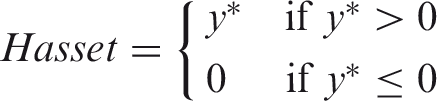
In contrast with income, the value of which is non-negative, household wealth can be negative due to financial liability. There are different ways to address the negative values of wealth as a dependent variable. Some researchers use net wealth as the dependent variable (e.g. Barsky et al., 2002; Smith, 1995; Yamokoski and Keister, 2006), thus allowing the existence of a negative value of wealth. Some researchers use Inverse Hyperbolic Sine (IHS) transformation (e.g. Meng, 2007). Other researchers model the positive and negative values separately (Killewald, 2013). Since wealth distribution is usually highly skewed, another commonly used method is log transformation. This requires the replacement of all negative values with a small positive number (Conley and Glauber, 2008; Hall and Crowder, 2011; Keister, 2003). In this study, we replaced all negative values with 0 and added 1 RMB to all outcome variables. We then take a log transformation of the dependent variable (wealth or income).
Equations (1) and (2) specify the models for household wealth or income.


Descriptive results of variables.
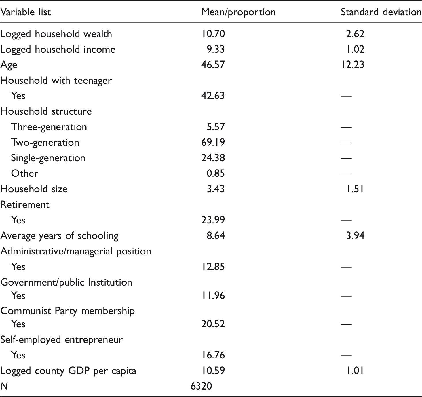
GDP: gross domestic product.
Censoring in wealth
To take a log transformation, we reset negative household wealth to zero, thus creating a censoring problem. Ideally, we need to model the zero and positive values separately. In our dataset, only 2.2% of households have negative wealth and thus take zero before the log transformation. We replicate our analysis using the ordinary least squares (OLS) regression with the Tobit model. However, the results of the Tobit model and OLS are identical. We thus choose to report the OLS results so as to simplify the discussion of the results.
When we decompose household wealth into housing assets and non-housing assets, a large portion of households have zero housing and non-housing assets (14.8% and 13.5%, respectively), which means censoring is non-negligible and we should model the zero and positive values separately. Following Wooldridge (2010), we applied the Tobit model to account for censoring. Specifically, we assume that there is a latent variable 
Coefficient comparison between wealth and income
Seemingly Unrelated Regression (SUR), proposed by Zellner (1962), is a special case of the linear regression model. SUR estimates two parallel regression equations simultaneously by assuming that the error terms are correlated, which can help gain efficiency in estimation by combining information on multiple equations as well as impose and/or test restrictions that involve parameters in different equations (Moon and Perron, 2006). Thus, it is possible to test whether a determinant has the same estimated coefficient in the wealth equation as in the income equation.
Results
Descriptive evidence
We first report model-free evidence about the relationship between household wealth and income. One widely accepted piece of wisdom about wealth and income is that household wealth inequality is larger than household income inequality (Keister, 2000, 2014; Morgan and Scott, 2007). For example, the economic inequality between different races is larger when measured with wealth than when measured with income (Menchik and Jianakoplos, 1997; Oliver and Shapiro, 1997). Similarly, according to the 2012 CFPS data, the Gini coefficient of net household wealth in China after adjustment is 0.73 (Xie and Jin, 2015),
2
while the Gini Coefficient of net household income is 0.53 (Xie and Zhou, 2014). Meanwhile, the 90/10 ratio for household wealth is 36.79, much higher than that for household income at 13.1 (Xie et al., 2013).
3
Using the CFPS data, we find that the Lorenz curve for wealth is apparently more rightly skewed than that for income, indicating much larger wealth inequality than income inequality, as shown in Figure 1.
Lorenz curve of household wealth and income.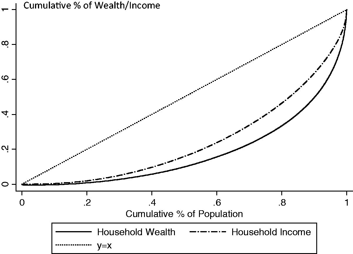
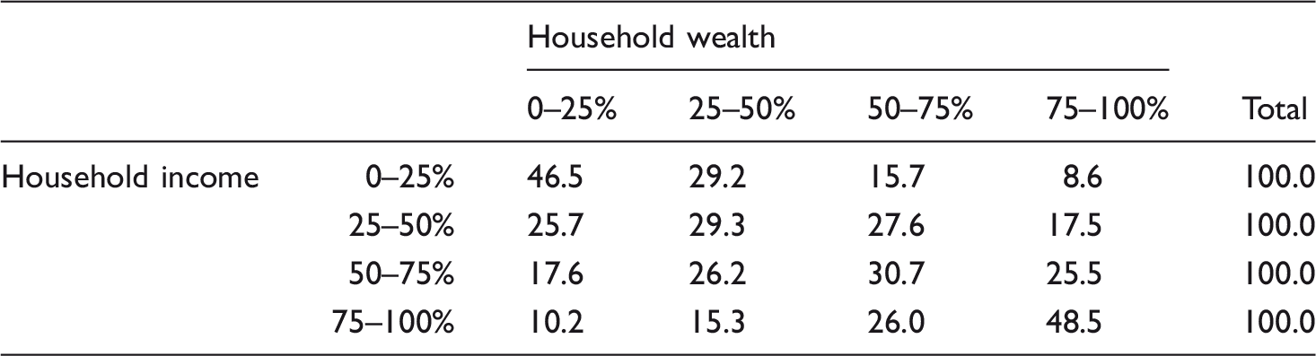
Distribution of household wealth and income (%).
In Figure 2, we plot the household wealth/income kernel density curve for people who work in government/public institutions and those who do not in order to illustrate the different distributions of wealth and income by political capital. From the figure, we observe the following: (1) households with members working in government/public institutions on average have higher wealth and incomes than households without such members; (2) both wealth and income distribution are more concentrated for households with members working in government/public institutions, indicating lower wealth and income inequality among these families than among those households without such members; (3) household wealth is more widely dispersed than household income, which means that wealth inequality overall is larger than income inequality.
Kernel density estimation of household wealth and income by work unit.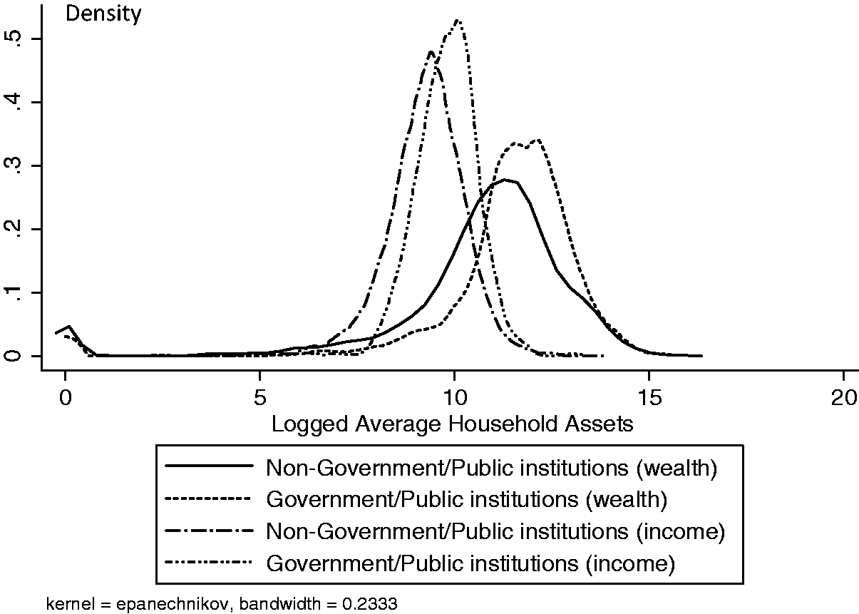
Household wealth and household income by political and market factors.
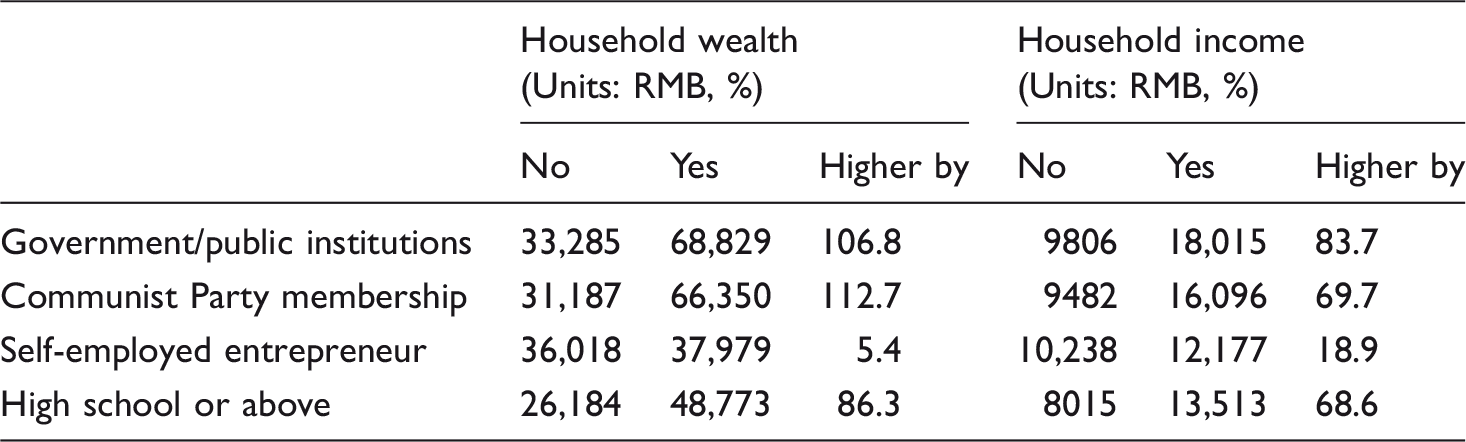
Note: Household wealth and income are weighted by the number of adults in a family, and sampling weights are used in the calculation.
For market factors, we have inconsistent findings: a self-employed entrepreneur enjoys a smaller premium in wealth (5.4%) than in income (18.9%), while the education gap (high school and above versus less than high school) is larger (86.3%) in wealth than in income (68.6%). However, we note that these observed patterns can be spurious without accounting for the fact that political capital may be selective with respect to human capital, such as education (Gerber, 2000). To sort out the net effects of market factors versus political factors, it is necessary to conduct a multivariate analysis with statistical models.
Regression model results
Seemingly Unrelated Regressions (SUR) of wealth and income.
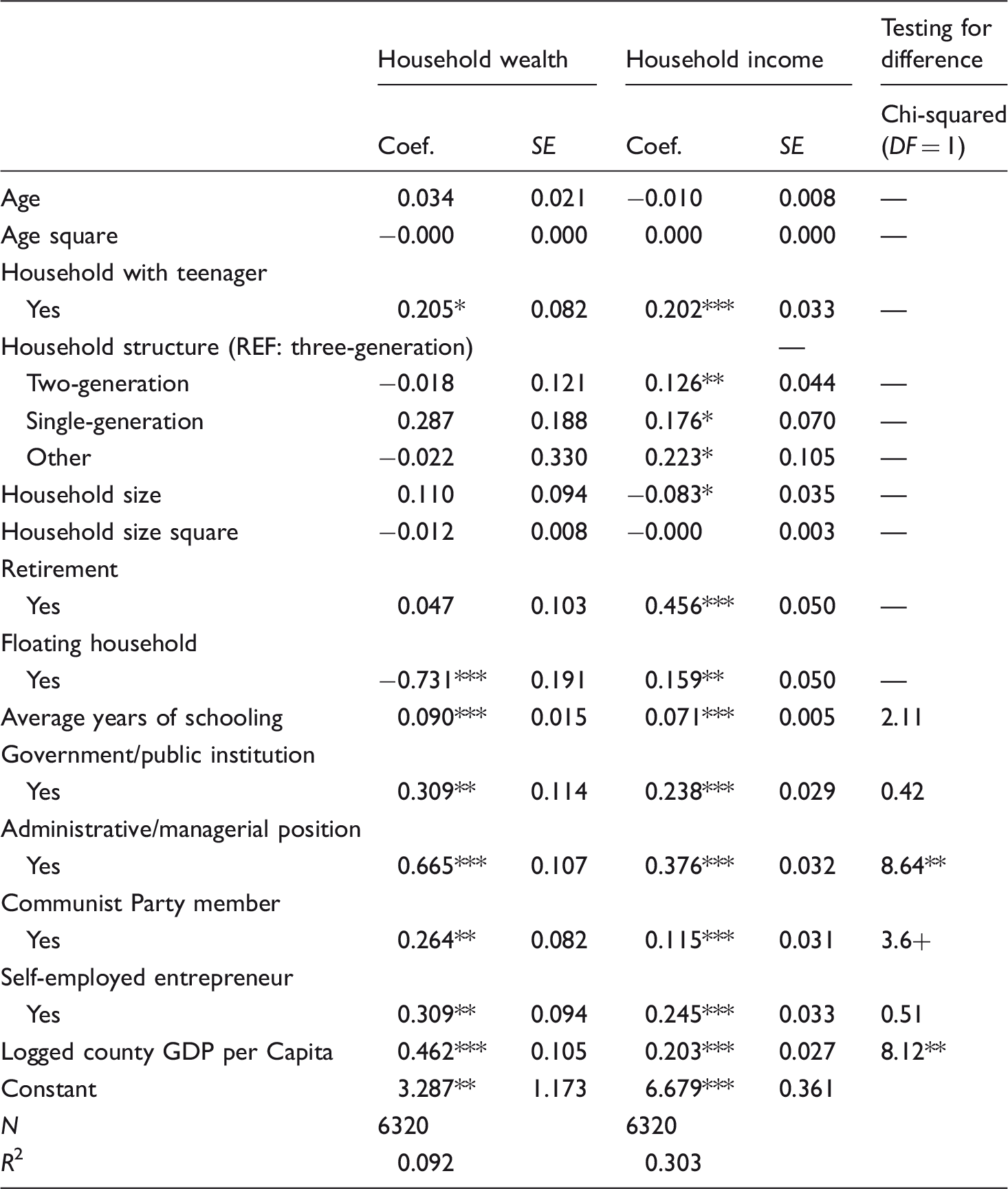
P < 0.001; **P < 0.01; *P < 0.05; +P < 0.1.
Notes: Standard errors were calculated with clustering at the county level; Coef. and SE denote coefficient and standard error, respectively; chi-squared statistic reported in the last column tests the statistical significance in the difference in coefficients between household wealth and household income.
GDP: gross domestic product.
From the regression results reported in Table 4, we observe a large positive association between years of schooling and household wealth. On average, an additional year of schooling is associated with a 9% increase in wealth. The wealth of households with a Communist Party member on average is 30% more than that of households with no Communist Party member, equivalent to the effect of a 2.9-year schooling increase, almost the difference between primary school and junior high school. By comparison, the party membership premium for income is 12%. Similarly, households with a member holding an administrative/managerial position enjoy a 94% advantage in wealth and 46% advantage in income. Working in government/public institutions on average is associated with a 36.2% increase in household wealth, the effect of which is equal to the effect of a 3.4-year schooling increase. These results confirm a common finding in the previous literature that political capital facilitates access to power and resources and thus leads to higher wealth and income (Bian and Logan, 1996; Hauser and Xie, 2005; Xie and Hannum, 1996; Zhou, 2000), as well as greater access to resources (Ma, 2011).
In our research, what is particularly interesting is that our regression analysis confirms the descriptive results: political capital has a larger effect on household wealth than on household income. We propose three speculative explanations for this. Firstly, political capital such as Communist Party membership may have helped households to acquire higher value housing properties with more square feet and better locations and amenities (Song and Xie, 2014; Walder and He, 2014) before the housing privatization reform. Rapid increases in housing prices since 2000 have amplified this advantage associated with favorable housing assignments conferred on households with higher political capital. Secondly, life expenses for households with high political capital may be lower than those for households with low political capital because of the better benefits (e.g. reimbursement, all kinds of subsidies) provided by their work units (Xie et al., 2009). Hence, with the same level of income, households with high political capital may be able to convert more income to wealth. Thirdly, households with high political capital may make financially more profitable investments thanks to their privileges in accessing policy information. At this point, we do not have sufficient data to evaluate the three propositions.
Some other studies have found that Communist Party membership had no significant effect on individual earnings when controlling for work unit and cadre status (Davis et al., 2005; Liu, 2005; Wu and Wu, 2009). Household income in our study is measured as the total income at the household level and takes all types of income into account, including wages, income from property and transfer payments. Our results show that Communist Party membership positively influences total household income in our data.
We also examine regional differences and the difference between floating and domestic households. It has been shown that regional differences play an important role in the level and inequality of household wealth. Xie and Jin (2015) found that 20% of the household wealth variation could be explained by region (i.e., provinces in their study). We show similar findings in Table 4. The level of economic development in a county has a significant positive and larger effect on household wealth compared with the effect on household income.
Previous studies have shown that the income of a floating population is not significantly different from the income of a domestic population. Zhou et al. (2013) found that floating populations have even higher incomes than domestic populations. However, floating households are at a disadvantage in terms of household wealth accumulation, as is shown in this study. Specifically, our results show that the wealth holdings of floating households on average are less than half (48%) those of domestic households. A possible explanation for this is that floating households cannot afford to purchase houses and sometimes face official barriers to doing so and, thus, possess less in the way of housing assets, to be shown in the later analysis. Since floating households do not own their own houses, a significant portion of their income is used to pay the rent, which further decreases household wealth accumulation. Also, it is relatively more difficult for floating individuals to invest in the financial market.
As for other control variables, the effects of household structure and household size on household wealth are statistically insignificant. Nevertheless, households with children under 15 years old tend to have higher household wealth. On the one hand, households with children under 15 years old have higher incomes, as evidenced by the income regression model. On the other hand, these household may have strong incentives to save for the future education and housing expenses of children.
Wealth decomposition
Tobit model of housing and non-housing assets.
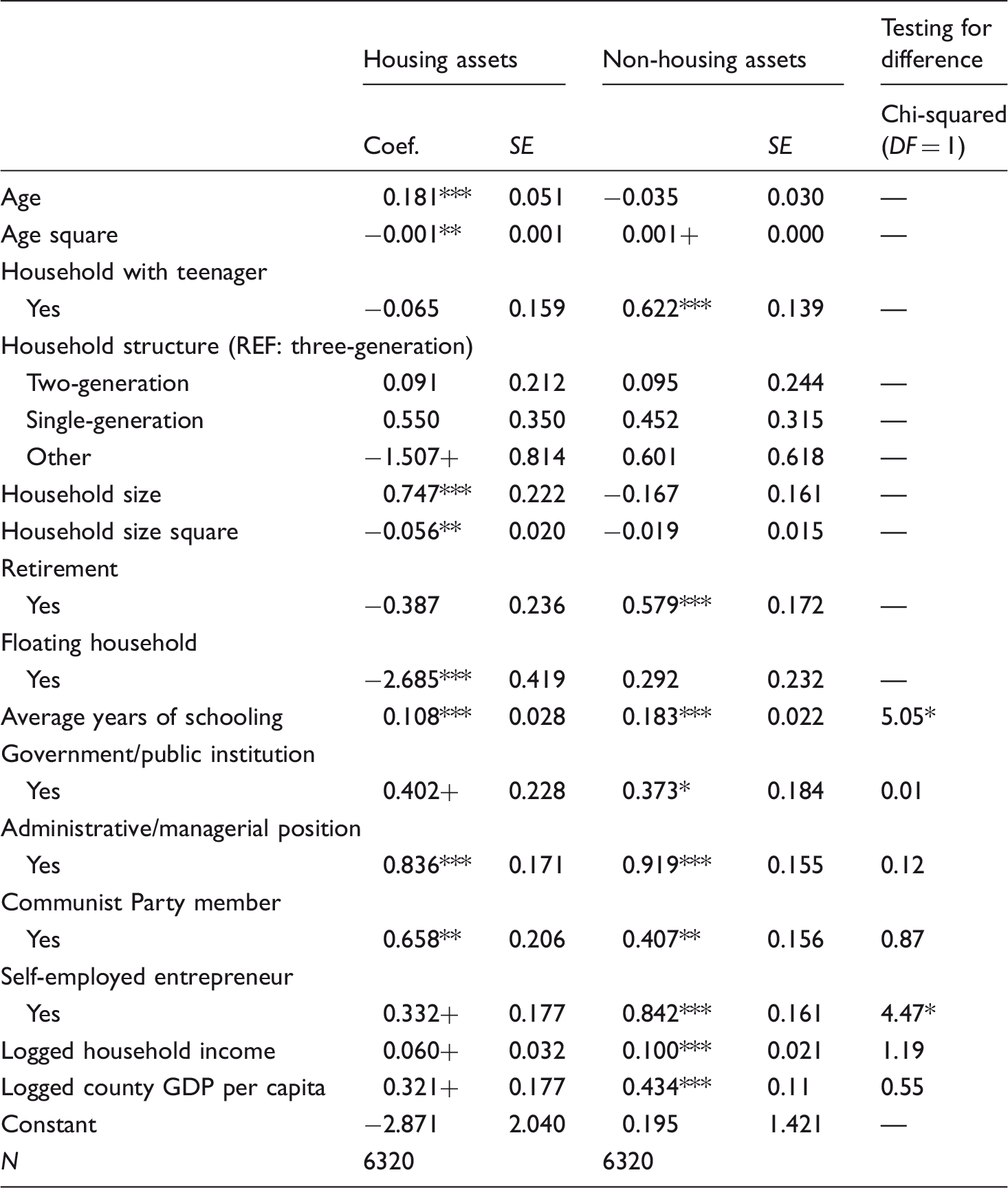
Note: Standard errors were calculated with clustering at the county level; Coef. and SE denote coefficient and standard error, respectively; chi-squared statistic reported in the last column tests the statistical significance in the difference in coefficients between housing and non-housing assets.
*** P < 0.001; **P < 0.01; *P < 0.05; +P < 0.1.
GDP: gross domestic product.
The results in Table 5 also confirm our earlier discussion that floating households are at a disadvantage concerning household wealth accumulation through housing assets, as the estimated coefficient suggests that their housing assets are only 7% of those possessed by local households. Their non-housing assets are no different from those of local households.
Causal pathways of political capital on household wealth
In this section, we discuss potential pathways through which political capital affects household wealth. We know that private wealth is a relatively recent phenomenon in China, resulting from sustained rapid growth after the economic reform that began in 1978 (Xie and Jin, 2015). Two processes have been responsible for generating wealth inequality: (a) political factors in the transition from a planned economy to a market economy and (b) market factors emerging in the market economy. Concrete mechanisms include housing, income, savings and investment. Given the short history of private wealth in China, legacy—one of the most important determinants of wealth in many other countries (Gale and Scholz, 1994)—does not play an obvious role in the process of household wealth accumulation in China. Below, we provide empirical evidence regarding how political capital may affect household wealth via housing assets, income, savings and investment returns.
Starting in the 1980s, the housing reform in China has helped urban families to obtain housing assets in an abrupt manner (Song and Xie, 2014; Walder and He, 2014), which has become the largest portion of household wealth (Xie and Jin, 2015). Do households with political capital have easier access to housing assets? We answer this question with data from the 2010 CFPS data. We show that 88.7% of the households with Communist Party membership have their own primary residence, 9.5% higher than households without Communist Party membership. Among households with Communist Party membership, 21.8% have other real estate properties compared with 16.9% among households without Communist Party membership. In addition, the homeownership rate for households with government/public institution employment is 88%, which ranks highest except for farming households. Furthermore, the ownership rate of other real estate properties for households with government/public institution employment is 23.5%, ranking second after households with a self-employed entrepreneur (Figure 3). In summary, we find that households with political capital are indeed more likely to own housing assets (home and other real estate) than those without it.
Rate of homeownership and other real estate by work unit.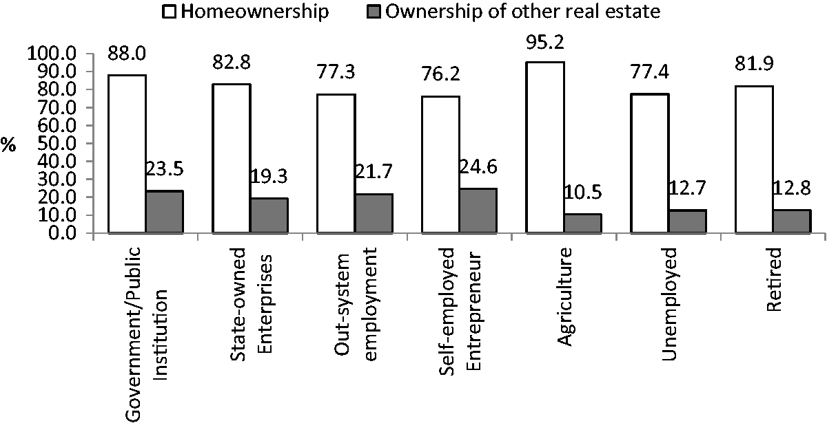
We already showed earlier, in Table 5, that political capital factors have positive effects on non-housing assets. In this section, we further investigate whether households with political capital have advantages in household accumulation, given the same level of income. In particular, we propose and try to provide evidence for two mechanisms: lower expenses and better investment.
Firstly, households with political capital (for example, working in a government/public institution) could have lower life expenses thanks to various kinds of allowances and welfare benefits, such as free or highly subsidized food, accommodation and transportation. Therefore, political capital may be associated with a larger portion of household income to be saved for wealth accumulation, given the same level of income. Secondly, households with a political capital advantage may have access to better financial and other investment opportunities. For example, households with political capital may be in better positions to acquire housing assets at discounted prices due either to their information or better social networks (also called guanxi).
In our CFPS data, we are unable to measure investment directly. To test our hypothesis in an indirect way, we predict the household financial assets to be an investment and expense outcome against household income, via a Tobit regression
4
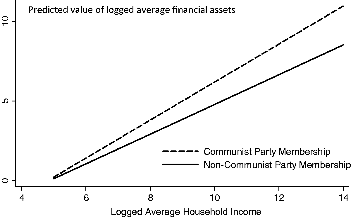
and plot the relationship by political factors, shown in Figures 4 and 5, with predicted logged household financial assets on the y-axis and log transformed household income on the x-axis. As shown in Figure 4, given the same level of household income, households with government/public institution employment have more financial assets compared with households without government/public service institute employment. Similarly, households with Communist Party membership also have more financial assets than households without Communist Party membership. These figures give some credence to the proposition that political capital may be associated with lower expenses and/or better investment. Actually, according to the CFPS data, households with the political capital advantage have relatively high education and entertainment expenses. The fact that households with political capital advantage have higher levels of savings suggests that a significant portion of their expenses may be reimbursed by their work units. Further research is needed to disentangle the effects of political capital through expenses versus investment pathways.
Predicted household financial assets by work unit conditional on household income. Predicted household financial assets by Communist Party membership conditional on household income.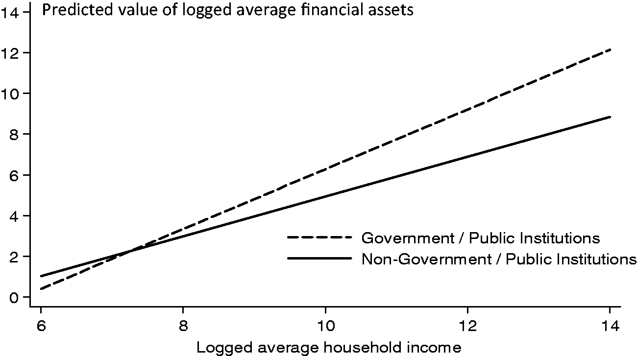
Conclusion
In this paper, we conducted a comparative analysis of the effects of political capital and market factors, as social determinants, on household wealth relative to household income. From descriptive and regression results, we draw four major conclusions as follows.
In urban China, families with political capital enjoy a greater wealth premium than income premium. We propose that housing assets, lower expenses due to benefits and allowances and higher investment returns are three main factors that contribute to the wealth accumulation advantage associated with political capital. Both political capital and market factors play important roles in the accumulation of household wealth. Households with government/public institution employment, Communist Party membership, a self-employed entrepreneur and higher average years of schooling have a significant advantage in household wealth accumulation. Political capital has a larger effect on housing assets than on non-housing assets, while market factors have a larger effect on non-housing assets than on housing assets. Regional disparity and hukou segregation are two structural factors that influence wealth accumulation, as well as income, in urban China.
This study has several limitations, which we acknowledge, as follows.
We have mainly used cross-sectional data from the CFPS and thus could not clearly differentiate the causal effects of political capital from those of market factors, as the two effects could be associated. For example, if an individual first worked in a government/public institution and then started his/her own business as an entrepreneur, the person’s business could benefit from his/her political connections. However, we do not know this from our data and thus cannot appropriately assign the importance of political capital to this person’s wealth accumulation as an entrepreneur. It may be possible to utilize longitudinal data, when the CFPS has enough waves in the future, for us to study detailed work history and disentangle the effects of political capital and market factors by tracing the lifetime wealth accumulation process. This approach would allow us to establish more credible causal links between political capital/market factors and household wealth. Due to the limitation of the survey data in the CFPS, we were not able to study extremely rich households, a common problem in studies of sampled data in wealth studies (Keister, 2000). The super-rich affect not only the level of wealth but also the distribution of wealth. In macro-level studies, researchers may use additional data to supplement sampled data for describing levels of wealth inequality (e.g. Xie and Jin, 2015). However, this approach is not applicable in a micro-level household wealth analysis. We know super-rich households include only a very small portion of the population and usually differ from households in the overall population. The focus of this study is on the average effects of political capital and market factors on household wealth. Therefore, omitting super-rich households should not significantly bias our statistical conclusions.
Footnotes
Acknowledgments
An early version of this article was originally published in Studies in Labor Economics 2015; 5: 4–27 (in Chinese).
Funding
This work was supported by the Natural Science Foundation of China (grant number 71373012), the Center on Contemporary China of Princeton University and the Center for Social Research of Peking University.