Sage Journals: Discover world-class research

Abstract

Background

Esophageal cancer is a major cause of cancer mortality, and accurate preoperative T staging guides treatment decisions. Conventional artificial intelligence approaches that rely on single-type data exhibit suboptimal accuracy in T-stage classification.

Objective

This study aimed to develop and validate a combined deep learning model for T-stage diagnosis by incorporating CT features and clinical variables.

Methods

About 443 EC patients who underwent postoperative pathological evaluation at three centers from 2018 to 2023 were included, with CT images, demographical information, and laboratory test results collected. Based on CT images, the hierarchical multiscale feature fusion network (HMFFN) extracted deep learning features, while three-dimensional reconstruction technology provided handcrafted morphologic features. Additionally, clinical features were obtained from clinical baseline data, laboratory tests, and endoscopic examination results. The auto-metric Graph Neural Network (AMGNN) was combined following the feature extraction module to fuse three types of features for T-stage classification.

Results

About 394 patients from internal datasets (mean [SD] age, 61.83 [7.42] years; 320 men [81.22%]) and 49 patients from external datasets (mean [SD] age, 62.84 [7.60] years; 41 men [83.67%]) were evaluated. Our proposed HMFFN-AMGNN model demonstrated excellent performance, achieving AUC of 0.848 (95%CI: 0.788–0.902) and 0.867 (95%CI: 0.792–0.929), as well as accuracy of 72.727% (95%CI: 62.121–83.333) and 77.551% (95%CI: 65.306–87.755) for internal and external test cohorts, respectively.

Conclusion

The combined deep learning model, integrating CT features with clinical variables, achieved high predictive precision in the diagnosis of EC T-stage, highlighting its potential to facilitate clinical decision-making.

Keywords

Deep learning esophageal cancer computed tomography imaging t-stage diagnosis feature fusion

Introduction

Esophageal cancer (EC) is the seventh most common cancer and the sixth leading cause of cancer-related deaths worldwide.^1,2 Of the EC cases, 59.2% occurred in East Asia and 53.7% occurred in China. Moreover, 58.7% of EC-related deaths occurred in East Asia, with China accounting for 55.3%.³ The overall social burden of EC should not be underestimated, especially as China is transitioning into an ageing society.^4–8 A great number of EC patients are diagnosed at advanced stages, necessitating prompt clinical intervention.^9,10 According to National Comprehensive Cancer Network (NCCN) guidelines, surgery is the principal treatment for EC patients. For instance, endoscopic submucosal dissection (ESD) or endoscopic mucosal resection (EMR) is recommended for T1-stage patients, whereas esophagectomy is the optimal therapeutic options for patients with locally advanced EC (T2 or T3).^11–15 Accurate preoperative T-staging in EC is critical for guiding surgical treatment and preventing delayed or excessive interventions.^16,17

Computed tomography (CT) with fine spatial resolution, which is good at presenting anatomical details and three-dimensional (3D) reconstruction, is widely employed for non-invasive local staging of EC.^17–19 Nevertheless, precisely determining the tumor T-stage using CT alone remains challenging for clinicians.^17,20–22 The accuracy highly depends on the level of their expertise, which easily leads to a large variance in the result interpretation and virtually reduces the work efficiency in medical decisions. With the rapid development of artificial intelligence (AI) methods in computer-aided diagnosis (CAD), the AI application can enhance patient management and clinical decision-making by bridging the knowledge gap in interpreting CT images and mitigating visual fatigue associated with image recognition.^23–25 Therefore, AI is crucial for identifying distinct tumor characteristics associated with different T stages.

However, previous studies have reported that the overall accuracy of traditional AI approaches for EC T-staging ranges from 60% to 69%.^26–28 These studies did not employ more advanced deep learning (DL) methods to make an improvement, while DL attained impressive performance in preoperative T-staging prediction tasks for gastric cancer,²⁹ rectal cancer,³⁰ nasopharyngeal carcinoma,³¹ or urothelial carcinoma.³² The main challenge is the lack of EC data for the DL model construction. Not only are specialized public imaging databases scarce, but it is also tough to collect medical images from EC patients whose T stage has been confirmed by the gold standard of postoperative pathological staging. To optimally leverage limited CT images for efficient feature extraction, transfer learning strategies were incorporated into the development of DL models.^33,34 To mitigate overfitting and enhance the generalization of DL features extracted from small CT datasets, we independently applied a 3D reconstruction model to CT imaging and extracted radiological features that capture morphological information relevant to tumor size, invasion depth, and spatial relationships with adjacent tissues factors central to the definition of tumor T-staging.^18,35

Integrating unstructured CT images and structured clinical data plays a critical role in uncovering diverse disease characteristics and providing a robust diagnosis.^36–38 It is conducive to building more stable and accurate clinical models, which are widely favored in different EC scenarios, including evaluating the therapeutic response,³⁹ assessing the risk of complications,⁴⁰ and predicting lymph node metastasis.⁴¹ However, only a few studies have attempted to combine unstructured and structured medical data to analyze tumor T-staging.⁴² Thus, this study also incorporated clinical features by collating the clinical records and fused them with DL and radiological features to precisely and reliably categorize the tumor T-stage.

Our research aimed to perform the T-stage diagnosis preoperatively in EC patients based on CT images and clinical data, developing and validating a novel and effective AI model. For this purpose, this study proposed a modular and integrated T-staging diagnostic framework centered on the combined DL model, leveraging CT features and clinical variables. It has the potential to evolve into a practical and valuable CAD tool, thereby facilitating the development of individualized treatment strategies in clinical practice.

Materials and methods

Patients enrollment and data collection

Patients who underwent radical EC surgery at Chongqing Southwest Hospital (institution 1) from January 2018 to April 2023 and Chongqing Cancer Hospital (institution 2) and People's Hospital of Chongqing Banan District (Institution 3) from January 2022 to August 2023 were retrospectively enrolled. Initially, we retrieved data of 691 patients from the hospital information system. CT images, demographical information, and laboratory test results of all patients were obtained from the electronic medical records. Inclusion criteria involved patients with (1) postoperative pathological confirmation of T-stage, (2) CT performed within 2 weeks before surgery, and (3) complete clinicopathological data and CT images. Patients were excluded if (1) clinicopathological data were inaccurate or missing, (2) CT image information was incomplete (e.g., the image lacked key parts such as the neck and gastroesophageal junction), (3) the diseased area was not obvious on CT images (i.e., tumor size <5 mm), or (4) the image quality was poor or artifacts were present.

T-staging was performed following the eighth edition of the American Joint Committee on Cancer (AJCC) TNM classification, categorized as T1, T2, T3, and T4.⁴³ Following the NCCN guidelines, T4-stage patients were excluded, as their treatment primarily involves neoadjuvant chemoradiotherapy rather than surgery.¹¹ Surgical intervention becomes appropriate only when tumors achieve downstaging from T4 to T1–T3. Therefore, including T4-stage patients does not align with the objective of preoperative prediction for facilitating surgical decisions. Besides, only few emergency salvage surgeries or less effective surgical treatments (such as R1–R2 resections) were performed in T4 patients. Consequently, the overall clinical value of surgery in T4 patients is limited, eliminating the need for preoperative diagnosis in these cases. Given the aims and clinical significance of our study design, we excluded T4 patients and focused on collecting data from patients at the T1–T3 stage. Finally, patients from institution 1 were randomly assigned to the training, validation, and test cohorts at a ratio of 4:1:1. Patients from Institutions 2 and 3 constituted an external test cohort to evaluate the effectiveness and feasibility of the diagnostic model (Figure 1). Our proposed T-staging diagnostic framework for EC patients is schematically presented in Figure 2. For this purpose, a hierarchical multiscale feature fusion network (HMFFN) was utilized to extract DL features from CT images,⁴⁴ while 3D reconstruction technology for CT imaging was applied to achieve radiological features. Clinical baseline data, laboratory tests, and endoscopic examination results were selected to obtain clinical features. These multisource features were fused using an auto-metric graph neural network (AMGNN) to realize the T-stage prediction.⁴⁵

Figure 1.

The flowchart of patient recruitment for this study.

Figure 2.

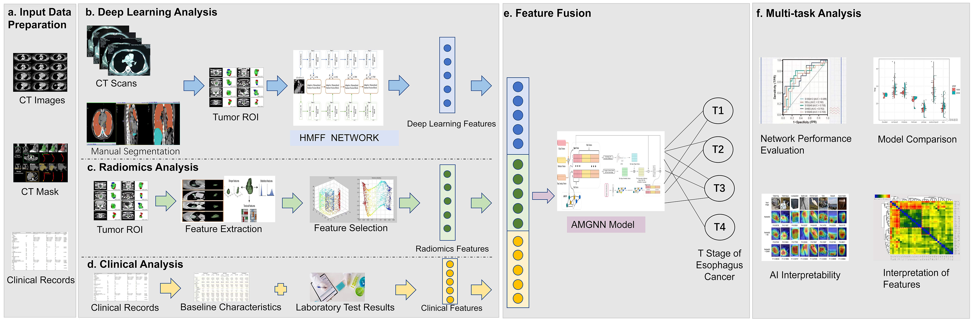
Overall workflow of study design. (a) Data preparation stage included collecting original CT image data, with manually labeled tumor images, patients’ baseline information and clinical examination report. (b) The pre-trained deep learning model architecture called hierarchical multiscale feature fusion network (HMFF Network) was used to extract features specifically for the small target region of interest (ROI) of esophageal cancer after parameter fine-tuning, and the deep learning features were obtained. (c) The pipeline of radiological analysis is the process that based on the three-dimensional reconstruction of esophageal cancer CT images, and the measured tumor morphological indicators are further screened and sorted to become radiological features. (d) Clinical characteristics considered comprehensive coverage of clinical information and were derived from manually extracted structured data from clinical patient baseline data and examination reports, respectively. (e) In the feature fusion step, meta metric graph neural network (AMGNN) was used to fully integrate deep learning features, radiological features and clinical features under the condition of small samples to generate multisource fusion features, and finally complete tumor T stage prediction. (f) Comprehensive evaluation of the developed joint model (HMFFN-AMGNN) In terms of the preoperative T staging prediction task for esophageal cancer.

CT acquisition

Original CT scans were performed on one of the two spiral CT scanners (64-detector Somatom Definition AS, Dual Source Somatom Definition Flash) or Sensation 16 at the three centers. CT acquisition parameters were set up as follows: Tube voltage, 100–120 kV; tube current, automatic set-up; pitch, 1.2–1.5 mm; reconstruction thickness, 2 mm; thickness interval, 2 mm. Reconstruction was performed on a soft tissue/mediastinal window (window level, 35∼40 HU; window width, 250∼300 HU). Before scanning, a voice prompted patients to cooperate with breath-holding to sup-press respiratory motion artefacts. An iodinated non-ionic contrast agent (iohexol, io-dine content of 300 mg/mL) was intravenously injected at a dosage of 1.7 mL/kg with a flow rate of 3.5–4.0 mL/s to acquire contrast-enhanced images. Continuous axial scanning was performed 10 s after injection. The arterial phase was delayed for 5 s when the CT value reached the trigger threshold (120 HU). The scan delay for venous-phase scanning was 15–20 s after the end of arterial-phase scanning.

DL feature extraction

Image segmentation

The original CT images in the DICOM format were uploaded to open-source Amira software (Version 6.0.0; http://www.thermofisher.com/amira-avizo). Two experienced cardiothoracic surgeons (C.J.C. and H.P.), who were blinded to clinical information and histopathological outcomes, manually segmented EC images to depict specific masks of the entire tumor, and delineate regions of interest (ROIs). They independently reviewed all CT images, reaching a consensus on interpretations through discussion. The segmented structures included tumor, esophagus, pericardium, aorta, bronchi, and lung, with labels created for these six structures. The ROIs, defined by bounding boxes marked by the doctors, encompassed the whole lesion area. All CT slices containing tumor ROIs were finely marked.

Image processing

The size of ROI was resampled to 56 × 56 pixels using bilinear interpolation and pixel values were normalized to the range of 0–100 before DL feature extraction, ensuring comparability in scale and spatial resolution among CT images from different hospitals. Data augmentation methods, such as horizontal flipping, random cropping, random rotation, and contrast transformation, were used after dataset splitting to reduce over-fitting in the training stage.

Model pre-training and fine-tuning

To compensate for the limited dataset size, 12,058 CT images from COVID-CTset dataset (https://github.com/mr7495/COVID-CTset) were utilized for our model pre-training. We loaded the model weight that represented the best pretraining results and employed the fine-tuning method to adjust the final modules and linear layers in the DL model using CT images of EC. In this way, the parameters of the preceding layers in the model were updated in advance to learn fundamental pixel-level information such as color, texture, edge, etc., and the remaining parameters were trained to capture more differentiated semantic information regarding the entire diseased area, which substantially reduced the amount of CT data required for model updating. During the pre-training phase on the COVID-19 CT image dataset, a binary classification task was implemented to distinguish between infected and non-infected individuals. The pretrained HMFFN was optimized using the cross-entropy loss function and the Adam Weight Decay Optimizer, with a learning rate of 0.0001 and a weight decay of 0.01.

Development of the DL model

The pre-trained DL model was helpful in learning deep high-dimensional features from CT images, and the HMFFN was applied to extract DL features (Figure 2(b)). Since the ROIs of EC manifests as small objects on CT images, applying a deep learning model to enhance the extraction of feature information for small target lesions is a critical step. For small target ROIs of EC, comprehensively learning and logically integrating both local and global features of ROIs are crucial, as this approach not only focuses on the local details of the diseased area but also considers the overall characteristics of the entire tumor.

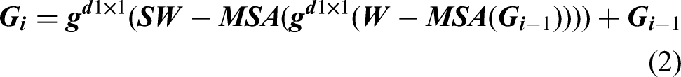
The overall model structure of CNN and Swin Transformer jointly extracting feature is shown in Figure 3(a). Both the local branch deep convolution network and the global branch Swin Transformer included four stages. Through the mutual adjustment of the convolution kernel and the number of windows, the size gap of the output feature dimension at each level was bridged, which was conducive to improving the effectiveness of the feature fusion module in the next step. Deep convolutional networks could effectively obtain local spatial content through convolution operations shown in formula (1), while Swin Transformer could extract global semantic information through the self-attention mechanism shown in formula (2).
$L_{i} = G E L U (M L P (f^{d 3 \times 3} (L_{i - 1}))) + L_{i - 1}$
(1)
$\begin{aligned} G_{i} = g^{d 1 \times 1} (S W - M S A (g^{d 1 \times 1} (W - M S A (G_{i - 1})))) + G_{i - 1} \end{aligned}$
(2)

Figure 3.
Overview of the pipeline of constructed joint model (HMFFN-AMGNN) based on CNN, Swin Transformer, meta-learning, metric learning, and GNN for classifying T staging of esophageal cancer. (a) Detailed structure of the HMFF network. The input was CT image of small target lesion area. After going through the multi-scale feature extraction by global feature module and local feature module and hierarchical feature fusion by adaptive feature fusion module, the output was deep learning features. (b) Specific details of the AMGNN model. The input was deep learning features, radiological features and clinical features. By means of reconstructing the multi-source fusion features via calculating the edge weight matrix and edge probability matrix and measuring the feature similarity relationship between sample nodes, the tumor T staging as output can be predicted accordingly. (c) Local feature block. (d) Global feature block. (e) Adaptive hierarchical feature fusion block.

Where $L_{i}$ denote the output features of the i-th local feature block, $G_{i}$ denote the output features of the i-th global feature block. $f^{d 3 \times 3}$ is the depthwise convolution operation with a convolution kernel size of 3 × 3, $g^{d 1 \times 1}$ is the linear operation with layer normalization. $M L P$ is Multilayer Perceptron and $G E L U$ is Gaussian Error Linear Unit. $W - M S A$ and $S W - M S A$ represent the Windows Multi-head Self-Attention module and Shift W-MSA module, respectively.

Since global features and local features played different roles in the prediction, the choice of branch parallel structure meant that local and global features could maintain integrity and independence to the greatest extent, assisting in building non-interfering feature maps through four stages. The adaptive hierarchical feature fusion module in the middle branch was applied to fuse local and global features of each stage. It is worth noting that when features were passed into the fusion module, the channel attention mechanism would be brought to global features, which improved the representation ability of global information, and spatial attention mechanism was applied to local features to magnify local details and suppress irrelevant regions. The specific calculation formulas of the adaptive hierarchical feature fusion module are as follows:
${\tilde{G}}_{i} = C A (G_{i}) \otimes G_{i}$
(3)
${\tilde{L}}_{i} = S A (L_{\dot{i}}) \otimes L_{i}$
(4)
${\tilde{F}}_{i} = f^{d 1 \times 1} (C o n c a t [G_{i}, L_{i}, A v g P o o l (f^{d 1 \times 1} (F_{i - 1}))])$
(5)
$F_{i} = I R M L P (C o n c a t [{\tilde{G}}_{i}, {\tilde{L}}_{i}, {\tilde{F}}_{i}]) + A v g P o o l (f^{d 1 \times 1} (F_{i - 1}))$
(6)

Where ${\tilde{G}}_{i}$ is the global features generated through the channel attention (CA) module, ${\tilde{L}}_{i}$ is the local features generated through the spatial attention (SA) module. ${\tilde{F}}_{i}$ is the result of concatenating global and local features of the current stage and the fusion of the previous stage. $F_{i}$ is the fusion feature generated in the current stage. $f^{d 1 \times 1}$ is the convolution operation with a convolution kernel size of 1 × 1. $A v g P o o l$ is the average pooling and $I R M L P$ is a residual inverted MLP. $\otimes$ represents the element-wise multiplication. Finally, the combined features from the fusion module in the fourth stage were exported to the fully connected layer, generating deep learning features.

The CPU used for training is Intel Xeon (R) Gold 6246R CPU @ 3.30 GHz, and the GPU is NVIDIA Tesla V100. In the whole network training cycle, the model was trained for a maximum of 300 epochs with early stopping and a fixed batch size of 16. The cross-entropy loss function and Adam Weight Decay Optimizer with a learning rate of 0.0001 and a weight decay of 0.01 were used.

Radiological feature extraction

To further enhance the robustness and clinical utility of CT imaging features extracted by DL, 3D reconstruction technique was adopted to quantify structural parameters from CT images (Figure 2(c)). It was developed to directly display the location, 3D morphology and spatial relationships for arteries, veins, nerves, lymph nodes and normal organs surrounding the tumor based on contrast-enhanced CT.^46,47 According to previous literature reports,^18,26 morphological characteristics that were highly correlated with EC T stages and of potential clinical significance were selected to form the final radiological features (Supplementary Table 1). The following pipeline steps were adopted for radiological feature extraction: (1) precise segmentation of the suspected tumor area, which was the same as the preprocessing used for DL feature extraction; (2) 3D reconstruction of EC and surrounding normal organs using well-segmented CT images, which was performed by stacking ROIs slice-by-slice to cover the entire tumor using Amira software (Supplementary Figure 1); and (3) calculation of the morphological parameters related to EC based on the 3D reconstruction model. The radiological feature extraction process was performed jointly by a cardiothoracic surgeon and a radiologist.

Clinical feature extraction

During the initial collection of clinical data, we incorporated insights from previous studies and integrated clinical practice to identify a comprehensive set of 27 variables potentially associated with T stages in EC. These variables were selected from multiple sources, including baseline clinical data, laboratory tests, endoscopic examinations, and histopathological examinations. Subsequently, strict statistical principles and significant clinical relevance were prioritized for secondary variable screening. The former adopted methods for handling missing values, variance filtering approach, Spearman correlation analysis, and univariate and multivariate logistic regressions, whereas the latter ascertained that selected features could exert a direct influence on the risk and progression of EC by referring to previous literature.^2,48–53 Specifically, the missing rate of variable values should be less than 50%, the threshold for variance filtering was set at 0.1, the correlation coefficient between variables should be less than 0.8, and the significance thresholds for univariate and multivariate logistic regression analyses were set at P < 0.05 and P < 0.001, respectively. Furthermore, usable clinical information must be available before EC surgery because the objective of this research emphasized the realization of preoperative T-staging diagnosis. Ultimately, the clinical variables that fulfilled the criteria were included as clinical features for model construction (Figure 2(d)). Supplemental Digital Content 2 and Supplementary Table 1 present the detailed process of clinical variable selection and the final clinical features, respectively.

For binary data such as gender, smoking history, and drinking history, categorical variables were converted into vectors of true values represented by 0 and 1. For the results of gastroscopy, the tumor location was divided into five categories including upper thoracic segment, middle upper thoracic segment, middle thoracic segment, middle lower thoracic segment, and lower thoracic segment by calculating the distance between the tumor and incisors. For continuous variables such as age and BMI, the Min-Max normalization method was applied to linearly transform the original data, and each index value was mapped to a vector format within the range of [0, 1].

Feature fusion model construction

The AMGNN was employed to integrate the DL, radiological, and clinical features (Figure. 2(e)). In the overall process of constructing the feature fusion model AMGNN (Figure 3(b)),⁴⁵ the first step was to initialize the small graph architecture which was mainly composed of a feature vector set, an edge probability matrix, and an edge weight matrix. We randomly selected a small number of labeled samples in each category and one unlabeled sample with their features as the feature vector set for model training. The features containing clinical information about risk factors, such as age, sex, smoking history, and drinking history, were used to calculate the edge probability matrix, as shown in formula (7). The numerical distribution of risk factors was regular and the feature dimension of them was low so that they could be directly utilized according to prior knowledge. Many studies have confirmed the relationship between risk factors and the subtyping of EC.^5,9,54
$e_{i, j} = 1 / (K + 1 - \sum_{1}^{K} e_{i, j}^{k}), e_{i, j}^{k} = {\begin{matrix} 1, i f | η_{i}^{k} - η_{j}^{k} | \leq β \\ 0, o t h e r w i s e \end{matrix}$
(7)

Where $e_{i, j}$ denotes the edge probability between the i-th and j-th node and is the element of the edge probability matrix in the i-th row and j-th column. K is the number of risk factors, and $η_{i}^{k}$ , $η_{j}^{k}$ represents the k-th risk factor feature of the i-th and j-th node. $β$ is the threshold to measure the similarity in the risk factor features between two nodes and represents prior knowledge.

Other features, which incorporated DL features, radiological features, and features related to laboratory tests or clinical records, had continuous numerical distributions and relatively high dimensionality. The measurement of the correlation between different samples based on these features cannot be directly defined, so learnable CNN was adopted to measure the similarity of the features mentioned above, which was automatically learned as an edge weight matrix, as shown in formula (8).
$w_{i, j} = CN N_{θ} (a b s (s_{i} - s_{j}))$
(8)

Where $w_{i, j}$ denotes the edge weight between the i-th and j-th node and is the element of the edge weight matrix in the i-th row and j-th column. $C N N_{θ}$ is a CNN network with updating parameter $θ$ . $a b s$ means absolute value, and $s_{i}$ , $s_{j}$ are other features of the i-th and j-th node. Finally, the metric connection matrix with probability constraints, which represented the similarity relationship between two sample nodes, could be obtained by multiplying these two matrices, and it was combined with a diagonal matrix forming the adjacency operator family to retain the features of the node itself when updating the node, as shown in formula (9).
$A = {D, E \otimes W}$
(9)

Where A is the adjacency operator family and D is the diagonal matrix. E is the edge probability matrix, and W is the edge weight matrix. $\otimes$ represents the element-wise multiplication. The nodes with close fusion features formed clusters by updating fusion features of the node using the operators in the adjacency operator family, and the categories of unknown nodes in the training set was outputted.

The first small graph structure of the AMGNN model was established through the above steps, and its updated parameters were used as initial parameters for starting training the subsequent same tasks similar to the meta-learning method. Each training iteration for the model parameters was completed with a small sample size. In the test phase, the model only needed a few known labeled samples as the source of label information and added an unknown sample to the test set to form a new graph. Soon, the well-trained AMGNN model outputted the category of this unknown node. The following hyperparameters were used: epochs, 600; mini-batch size, 2; learning rate, 0.0001; weight decay, 0.01; cross entropy loss function; Adam Weight Decay Optimizer.

Comparisons of model performance with classical AI methods and surgical doctors

Among the three kinds of features, CF was derived from structured clinical variables, and RF came from structured calculation data about the tissue and organ morphology in CT images after 3D reconstruction, while DF was extracted from the unstructured ROIs of CT images. In order to prove that our diagnostic model has advantages in processing unstructured CT images and structured clinical variables, we selected various classical models suitable for two types of raw data to make comparisons, respectively. Our study utilized the HMFFN for processing unstructured CT images and outputting DL features, so DL models related to CNN or Transformer with a similar structure were selected to be compared. The model inputs were the ROIs of CT images when using unstructured data. The AMGNN model was used to fuse structured data feature in our research, and traditional machine learning methods commonly adopted in analyzing structured data were chosen here for comparison. The classical machine learning algorithms employed in this study include Support Vector Machine, Logistic Regression, K-Nearest Neighbors, Naive Bayes, Random Forest, and Multi-Layer Perceptron. The model inputs were radiological and clinical features when using structured data. All hyperparameters were kept consistent and set as follows: epochs, 600; mini-batch size, 2; learning rate, 0.0001; weight decay, 0.01; cross entropy loss function; Adam Weight Decay Optimizer; test size splits, 0.2; random state, 0; stratify, none; the number of bootstrap replicates, 1000.

Additionally, the patients were randomly sampled from our internal dataset in three batches of 100 patients each. During the sampling process, we ensured via Python programming that approximately 30 cases were selected from each of the T1 to T3 stages to achieve category balance and effectively avoid selection bias. Based on their clinical records and CT images, three clinicians with different experience levels (junior, intermediate, and senior doctors) were requested to determine T-staging diagnoses for comparison with our proposed model to assess practical clinical benefits. Specifically, junior doctors were defined as those with 3 years of clinical experience in thoracic EC, while intermediate and senior doctors had 8 and 10 years of clinical experience in EC, respectively.

Statistical analysis

When comparing patients’ baseline data, Pearson's chi-squared test, Fisher's exact test, or Kruskal–Wallis H test was employed to compare differences in categorical variables, whereas one-way analysis of variance was used to compare differences in continuous variables. The area under the receiver operating characteristic (ROC) curve (AUC), accuracy (ACC), precision (PRE), recall (REC), and F1-score were calculated to evaluate the discrimination performance of T-staging predictions. Bootstrap test technology was employed to estimate the 95% confidence interval (CI) of all the indices. Both macro-AUC and micro-AUC were investigated to draw ROC curves for multi-classification. Decision curve analysis (DCA) showed the clinical utility of the model. The Gradient-weighted Class Activation Mapping (Grad-CAM) technique was applied to calculate the importance of each pixel to a specific category by the gradient backpropagation of the network, thereby visualizing the salient lesion regions identified by the DL model. The Uniform Manifold Approximation and Projection (UMAP) method was adopted to illustrate the overall prediction performance by converting the DL features into color-coded representations of the T1–T3 stages. All statistical tests were two-tailed, with P < 0.05 considered statistically significant. All statistical analyses were performed using IBM SPSS Statistics 25 (Armonk, New York, USA) and R 4.1.0 (http://www.R-project.org). The models were implemented using toolkits of Pytorch V.1.9.0 and Python 3.9.13 (https://www.python.org/).

Results

Clinical characteristics

Table 1 summarizes the clinicopathological characteristics of eligible EC patients in the internal dataset (n = 394; T1 = 102 [25.89%], T2 = 158 [40.10%], T3 = 134 [34.01%]) and the independent external dataset (n = 49; T1 = 12 [24.49%], T2 = 17 [34.69%], T3 = 20 [40.82%]). Most patients were men, and the mean age of the EC patients was over 60 years. Squamous cell carcinoma was the most common histological type. No significant differences were observed in any of the eight clinical baseline data among the four cohorts (P > 0.05).

Table 1.
Demographic and clinical characteristics of esophageal cancer patients stratified by T stages in the training, validation, internal test, and external test cohorts.

Characteristic Internal dataset (Institution 1, n = 394) External dataset (Institutions 2 and 3, n = 49) P-value

Train cohort (n = 263) Validation cohort (n = 65) Test cohort (n = 66) Test cohort (n = 49)

T1 T2 T3 T1 T2 T3 T1 T2 T3 T1 T2 T3

Age, mean (SD), year 61.95 (7.64) 61.68 (7.00) 61.82 (7.77) 62.47 (6.72) 63.76 (7.18) 60.43 (9.28) 60.47 (5.56) 62.24 (6.39) 64.21 (8.74) 61.67 (8.98) 63.53 (7.45) 62.95 (7.16) 0.577

Gender, n (%) 66 (100.00) 108 (100.00) 89 (100.00) 19 (100.00) 25 (100.00) 21 (100.00) 17 (100.00) 25 (100.00) 24 (100.00) 12 (100.00) 17 (100.00) 20 (100.00) 0.294

Male, n (%) 50 (76.76) 86 (79.63) 71 (79.78) 14 (73.68) 22 (88.00) 19 (90.48) 12 (70.59) 24 (96.00) 22 (91.67) 10 (83.33) 15 (88.24) 16 (80.00)

Female, n (%) 16 (24.24) 22 (20.47) 18 (20.22) 5 (26.32) 3 (12.00) 2 (9.52) 5 (29.41) 1 (4.00) 2 (8.33) 2 (16.67) 2 (11.76) 4 (20.00)

BMI, mean (SD) 22.77 (2.88) 23.17 (2.89) 22.81 (3.26) 23.83 (2.29) 22.76 (1.50) 21.92 (3.14) 23.90 (4.58) 21.23 (2.06) 22.42 (2.59) 23.83 (3.21) 22.70 (3.40) 24.15 (3.97) 0.191

TNM stage, n (%) 66 (100.00) 108 (100.00) 89 (100.00) 19 (100.00) 25 (100.00) 21 (100.00) 17 (100.00) 25 (100.00) 24 (100.00) 12 (100.00) 17 (100.00) 20 (100.00) 0.082

Ⅰ, n (%) 59 (89.39) 10 (9.26) 0 (0.00) 16 (84.21) 3 (12.00) 0 (0.00) 16 (94.12) 0 (0.00) 0 (0.00) 8 (66.67) 3 (17.65) 0 (0.00)

Ⅱ, n (%) 6 (9.09) 68 (62.96) 58 (65.17) 3 (15.79) 17 (68.00) 12 (57.14) 1 (5.88) 15 (60.00) 15 (62.50) 2 (16.67) 7 (41.18) 7 (35.00)

Ⅲ, n (%) 1 (1.52) 29 (26.50) 26 (29.21) 0 (0.00) 4 (16.00) 8 (38.10) 0 (0.00) 10 (40.00) 9 (37.50) 0 (0.00) 6 (35.29) 11 (55.00)

Ⅳ, n (%) 0 (0.00) 1 (0.93) 5 (5.62) 0 (0.00) 1 (4.00) 1 (4.76) 0 (0.00) 0 (0.00) 0 (0.00) 2 (16.67) 1 (5.88) 2 (10.00)

Histology, n (%) 66 (100.00) 108 (100.00) 89 (100.00) 19 (100.00) 25 (100.00) 21 (100.00) 17 (100.00) 25 (100.00) 24 (100.00) 12 (100.00) 17 (100.00) 20 (100.00) 0.362

SCC, n (%) 65 (98.48) 105 (97.22) 88 (98.88) 18 (94.74) 25 (100.00) 20 (95.24) 15 (88.24) 25 (100.00) 23 (95.83) 12 (100.00) 17 (100.00) 20 (100.00)

Non-SCC, n (%) 1 (1.52) 3 (2.78) 1 (1.12) 1 (5.26) 0 (0.00) 1 (4.76) 2 (11.76) 0 (0.00) 1 (4.17) 0 (0.00) 0 (0.00) 0 (0.00)

Tumor location under gastroscopy, n (%) 66 (100.00) 108 (100.00) 89 (100.00) 19 (100.00) 25 (100.00) 21 (100.00) 17 (100.00) 25 (100.00) 24 (100.00) 12 (100.00) 17 (100.00) 20 (100.00) 0.955

Upper segment, n (%) 7 (10.61) 8 (7.41) 12 (13.48) 2 (10.53) 1 (4.00) 2 (9.52) 2 (11.76) 0 (0.00) 2 (8.33) 1 (8.33) 1 (5.88) 2 (10.00)

Middle and upper segment, n (%) 4 (6.06) 13 (12.04) 6 (6.74) 0 (0.00) 1 (4.00) 3 (14.29) 2 (11.76) 1 (0.04) 3 (0.125) 1 (8.33) 1 (5.88) 3 (15.00)

Middle segment, n (%) 30 (45.45) 35 (32.41) 26 (29.21) 10 (52.63) 13 (52.00) 5 (23.81) 8 (47.06) 9 (0.36) 11 (45.83) 4 (33.33) 8 (47.06) 7 (35.00)

Middle and lower segment, n (%) 9 (13.64) 21 (19.44) 16 (17.98) 1 (5.26) 4 (16.00) 4 (19.05) 3 (17.65) 6 (0.24) 3 (0.125) 4 (33.33) 3 (17.65) 3 (15.00)

Lower segment, n (%) 16 (24.24) 31 (28.70) 29 (32.58) 6 (31.58) 6 (24.00) 7 (33.33) 2 (11.76) 9 (0.36) 5 (20.83) 2 (16.67) 4 (23.53) 5 (25.00)

Smoking status, n (%) 66 (100.00) 108 (100.00) 89 (100.00) 19 (100.00) 25 (100.00) 21 (100.00) 17 (100.00) 25 (100.00) 24 (100.00) 12 (100.00) 17 (100.00) 20 (100.00) 0.272

Former, n (%) 40 (60.61) 68 (62.96) 59 (66.29) 11 (57.89) 18 (72.00) 13 (61.90) 8 (47.06) 22 (88.00) 18 (75.00) 8 (66.67) 10 (58.82) 10 (50.00)

Never, n (%) 26 (39.39) 40 (37.04) 30 (33.71) 8 (42.11) 7 (28.00) 8 (38.10) 9 (52.94) 3 (12.00) 6 (25.00) 4 (33.33) 7 (41.18) 10 (50.00)

Drinking status, n (%) 66 (100.00) 108 (100.00) 89 (100.00) 19 (100.00) 25 (100.00) 21 (100.00) 17 (100.00) 25 (100.00) 24 (100.00) 12 (100.00) 17 (100.00) 20 (100.00) 0.313

Former, n (%) 38 (57.58) 68 (62.96) 60 (67.42) 11 (57.89) 14 (56.00) 13 (61.90) 7 (41.18) 20 (80.00) 17 (70.83) 3 (25.00) 11 (64.71) 10 (50.00)

Never, n (%) 28 (42.42) 40 (37.04) 29 (32.58) 8 (42.11) 11 (44.00) 8 (38.10) 10 (58.82) 5 (20.00) 7 (29.17) 9 (75.00) 6 (35.29) 10 (50.00)

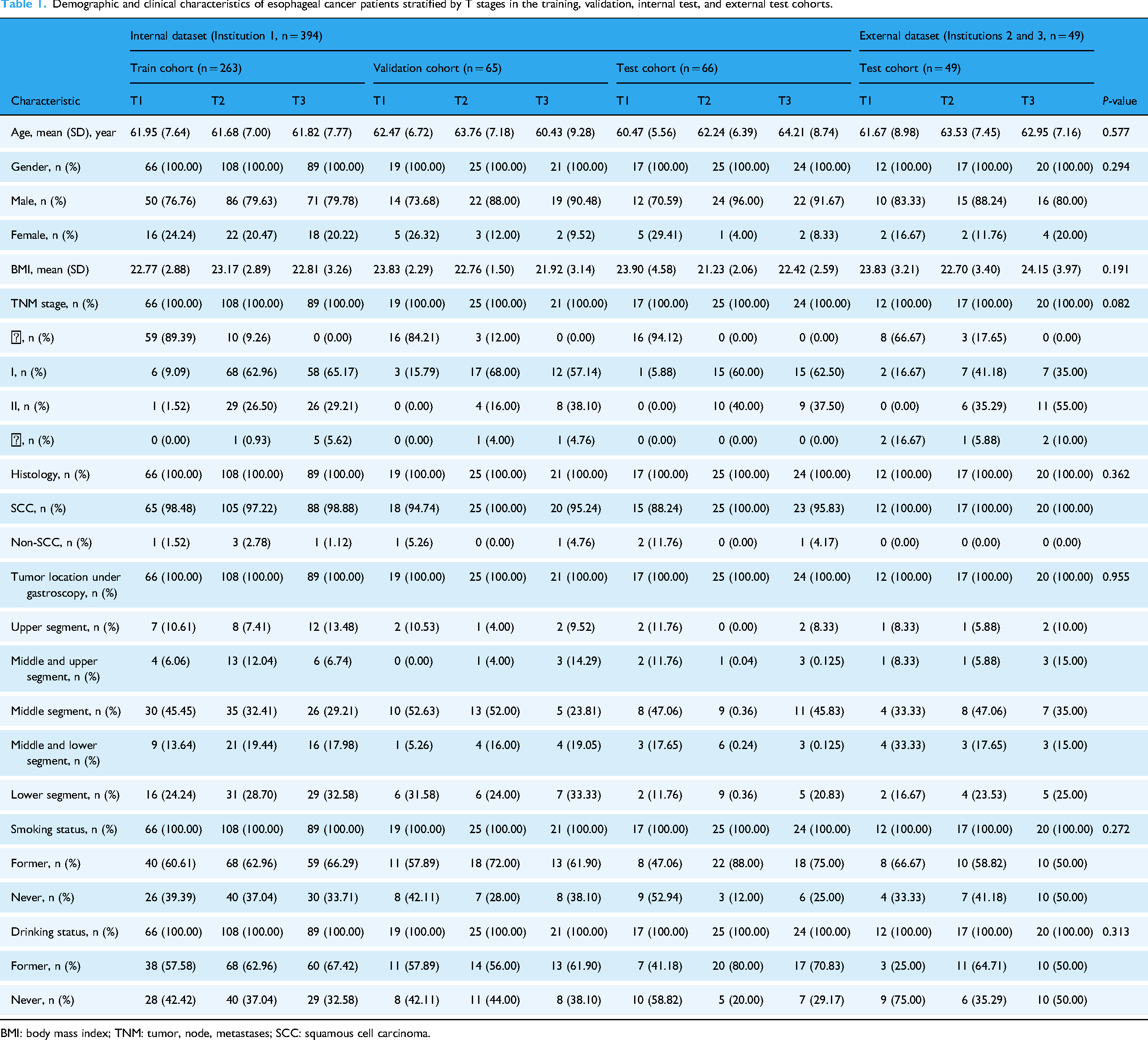
BMI: body mass index; TNM: tumor, node, metastases; SCC: squamous cell carcinoma.

Model performance under different feature combinations

The impact of different feature combinations on the prediction performance was analyzed on the basis of deep learning features (DF), radiological features (RF), and clinical features (CF) (Tables 2 and 3). In the internal cohort, the model test results demonstrated that the highest ACC (71.212%, 95%CI: 60.606–81.818) was observed in RF, and the lowest (59.091%, 95%CI: 46.970–71.212) was from CF when using a single feature. Similar phenomena were observed in the external test cohort, showing that the ACC was 69.388% (95%CI: 57.143–81.633) based on RF and 61.224% (95%CI: 46.939–73.469) based on CF. Model performance improved when RF or CF was fused with DF. The AUC of RF + DF or CF + DF in both cohorts reached over 0.75, and the values of ACC, PRE, REC, and F1-score in the independent test cohort improved to over 65%. The best prediction performance was achieved by fusing DF, RF, and CF, which was reflected as 0.848 (95%CI: 0.788–0.902) in AUC and 72.727% (95%CI: 62.121–83.333) in ACC for the internal test dataset, and 0.867 (95%CI: 0.792–0.929) in AUC and 77.551% (95%CI: 65.306–87.755) in ACC for the external test dataset.

Table 2.
Predictive performance of T staging for esophageal cancer using different feature combinations in the internal test cohort.

Data characteristics AUC (95% CI) Accuracy (95% CI) Precision (95% CI) Recall (95% CI) F1-score (95% CI)

DF 0.787 (0.721–0.852) 60.606 (50.000–72.727) 62.673 (51.634–73.765) 60.185 (48.350–72.258) 61.406 (48.627–71.605)

RF 0.774 (0.696–0.844) 71.212 (60.606–81.818) 49.487 (42.708–55.607) 56.066 (49.376–61.875) 51.759 (44.708–57.621)

CF 0.716 (0.633–0.794) 59.091 (46.970–71.212) 43.160 (35.000–50.556) 54.895 (47.874–61.209) 46.712 (38.840–53.333)

DF + RF 0.800 (0.731–0.860) 62.121 (50.000–72.727) 54.215 (37.771–78.413) 53.694 (45.040–63.154) 50.148 (40.256–61.396)

DF + CF 0.785 (0.715–0.852) 65.152 (53.030–75.758) 68.950 (56.734–80.139) 67.210 (57.729–76.389) 63.933 (51.499–74.680)

RF + CF 0.776 (0.704–0.844) 66.667 (54.545–77.273) 46.090 (38.636–53.301) 52.533 (45.086–59.249) 48.340 (40.507–54.988)

DF + RF + CF 0.848 (0.788–0.902) 72.727 (62.121–83.333) 72.839 (59.911–84.803) 69.559 (58.782–80.159) 69.665 (57.361–80.317)

DF: deep learning feature; RF: radiological feature; CF: clinical feature.

Table 3.
Predictive performance of T staging for esophageal cancer using different feature combinations in the external test cohort.

Data characteristics AUC (95% CI) Accuracy (95% CI) Precision (95% CI) Recall (95% CI) F1-score (95% CI)

DF 0.742 (0.644–0.828) 63.265 (48.980–75.510) 39.591 (30.476–48.810) 48.659 (37.582–58.774) 43.193 (33.048–52.125)

RF 0.802 (0.723–0.876) 69.388 (57.143–81.633) 46.825 (38.492–55.159) 59.649 (52.747–65.217) 52.199 (44.806–58.602)

CF 0.681 (0.583–0.778) 61.224 (46.939–73.469) 73.704 (32.222–81.878) 52.337 (40.000–63.248) 50.271 (35.973–63.313)

DF + RF 0.794 (0.703–0.877) 71.429 (59.184–83.673) 65.236 (51.410–80.152) 65.369 (51.157–80.471) 65.243 (50.859–79.199)

DF + CF 0.756 (0.661–0.842) 67.347 (55.102–79.592) 73.333 (62.654–84.188) 65.377 (51.323–78.430) 65.043 (49.750–77.914)

RF + CF 0.709 (0.607–0.798) 65.306 (51.020–77.551) 44.841 (36.201–53.125) 56.000 (49.425–61.905) 47.893 (38.760–55.295)

DF + RF + CF 0.867 (0.792–0.929) 77.551 (65.306–87.755) 77.908 (66.071–89.019) 77.895 (65.765–89.072) 77.731 (65.074–88.333)

DF: deep learning feature; RF: radiological feature; CF: clinical feature.

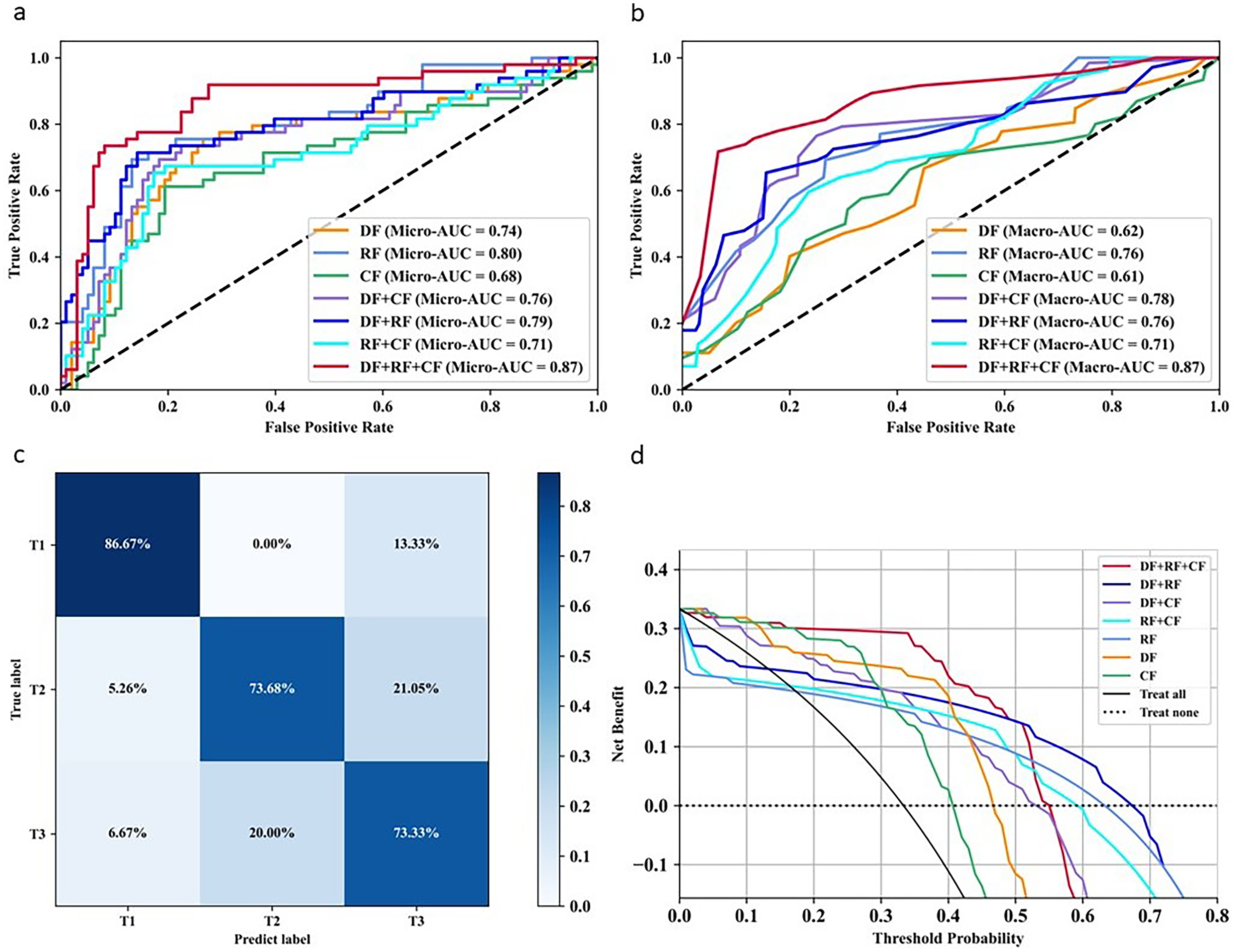
The ROC curve based on macro-AUC and micro-AUC (Figures 4(a)–(b) and 5(a)–(b)) demonstrated that our proposed model combining DF, RF, and CF yielded the best classification performance for the internal and external test sets. The confusion matrix illustrating the optimal model performance (Figures 4(c) and 5(c)) indicated that the T1-stage predictions achieved the highest ACC, exceeding 80%, whereas the T3-stage predictions showed the lowest ACC. The clinical benefit analysis (Figures 4(d) and 5(d)) indicated that our model incorporating DF, RF, or CF significantly enhanced preoperative T-staging assessment in EC compared with default strategies (such as treat all or treat none).

Figure 4.
Model performance in predicting T staging of esophageal cancer using different feature combinations in the internal test cohort. (a) and (b) ROC of different feature combinations based on macro-AUC and micro-AUC, respectively. (c) Confusion matrix calculated from model classification results combining DF, RF, and CF. (d) Decision curve analysis based on different feature combinations.

Figure 5.
Model performance in predicting T staging of esophageal cancer using different feature combinations in the external test cohort. (a) and (b) ROC of different feature combinations based on macro-AUC and micro-AUC, respectively. (c) Confusion matrix calculated from model classification results combining DF, RF, and CF. (d) Decision curve analysis based on different feature combinations.

Comparisons of model performance to classical methods

The results of the performance comparison with structured and unstructured data were shown in Tables 4 and 5 respectively. The prediction results demonstrated that HMFFN showed the best performance with the AUC reaching 0.787 (95% CI: 0.721–0.852) and the remaining evaluation indexes reaching over 60%. Similarly, AUC and ACC obtained by the AMGNN model were much better, while PRE, SEN, and F1-score were all lower than those of the Random Forest method, and PRE performance was even worse than that of K-Nearest Neighbor and Naïve Bayes.

Table 4.
Predictive performance comparison of the HMFFN to different models using unstructured CT images.

Methods AUC (95% CI) Accuracy (95% CI) Precision (95% CI) Recall (95% CI) F1-score (95% CI)

ConvNeXt-T 0.600 (0.515–0.683) 40.000 (27.692–52.308) 29.894 (10.256–49.180) 35.294 (33.333–39.583) 22.448 (15.447–30.527)

Resnet-34 0.606 (0.525–0.690) 44.615 (32.308–56.923) 45.723 (31.588–59.957) 43.311 (30.982–55.693) 43.442 (30.334–55.342)

EfficientNet-B0 0.638 (0.559–0.716) 43.077 (30.769–55.385) 48.201 (34.066–61.430) 42.142 (29.789–54.020) 43.361 (30.166–55.300)

Swin transformer-T 0.613 (0.534–0.694) 43.077 (30.769–55.385) 47.778 (26.796–64.141) 40.955 (29.499–52.778) 39.646 (26.299–52.433)

T2T-ViT_t-24 0.638 (0.563–0.718) 40.000 (27.692–52.308) 46.061 (21.494–69.444) 36.781 (27.895–46.019) 31.353 (19.337–43.111)

HMFFN-AMGNN (DF) 0.787 (0.721–0.852) 60.606 (50.000–72.727) 62.673 (51.634–73.765) 60.185 (48.350–72.258) 61.406 (48.627–71.605)

HMFFN-AMGNN (DF + RF + CF) 0.848 (0.788–0.902) 72.727 (62.121–83.333) 72.839 (59.911–84.803) 69.559 (58.782–80.159) 69.665 (57.361–80.317)

DF: deep learning feature; RF: radiological feature; CF: clinical feature.

Table 5.
Predictive performance comparison of the AMGNN to different models using structured clinical data.

Methods AUC (95% CI) Accuracy (95% CI) Precision (95% CI) Recall (95% CI) F1-score (95% CI)

Support vector machine 0.680 (0.602–0.755) 41.791 (29.851–55.224) 40.980 (27.408–55.662) 39.970 (28.932–51.346) 38.462 (26.607–50.831)

Logistic regression 0.677 (0.601–0.753) 43.284 (31.343–55.224) 41.852 (30.263–53.947) 43.727 (32.660–55.525) 42.445 (31.028–53.326)

K-nearest neighbor 0.701 (0.630–0.771) 49.254 (37.313–61.194) 50.397 (37.947–63.145) 49.364 (37.065–61.648) 49.781 (37.155–61.306)

Naïve Bayes 0.709 (0.634–0.782) 49.254 (37.313–61.194) 47.196 (34.454–60.804) 50.121 (40.058–60.790) 46.514 (34.964–58.052)

Random forest 0.739 (0.668–0.806) 53.731 (41.791–65.672) 54.095 (42.271–65.523) 53.727 (42.320–65.870) 53.890 (41.857–64.665)

Multilayer perceptron 0.708 (0.631–0.783) 46.269 (34.328–58.209) 44.433 (31.159–58.283) 47.758 (36.928–58.394) 43.495 (32.305–54.219)

HMFFN-AMGNN (RF + CF) 0.776 (0.704–0.844) 66.667 (54.545–77.273) 46.090 (38.636–53.301) 52.533 (45.086–59.249) 48.340 (40.507–54.988)

HMFFN-AMGNN (DF + RF + CF) 0.848 (0.788–0.902) 72.727 (62.121–83.333) 72.839 (59.911–84.803) 69.559 (58.782–80.159) 69.665 (57.361–80.317)

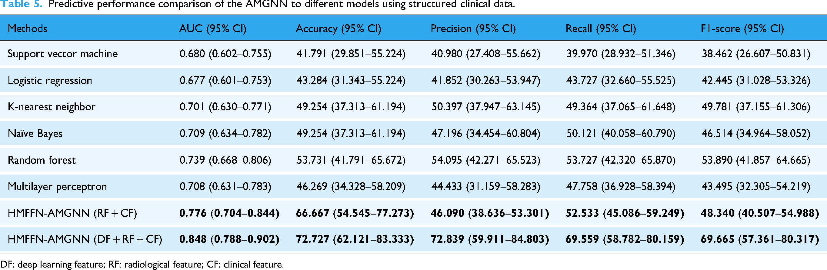
DF: deep learning feature; RF: radiological feature; CF: clinical feature.

Comparisons of diagnostic performance between surgical clinicians and the model HMFFN-AMGNN

Table 6 and Figure 6 present the T-staging prediction results from the three clinicians and the model HMFFN-AMGNN. The senior surgeon exhibited superior performance in T-stage recognition, with an AUC of 0.715 (95%CI: 0.661–0.770) and an ACC of 62% (95% CI: 52–71); however, a nearly 10% gap in predictive performance existed between the best clinician and our proposed model. Furthermore, the confusion matrix results (Figures 4(c), 5(c), and 6(c)–(e)) revealed that the model surpassed the intermediate clinician in identifying each T-stage, even reaching the level of senior doctors in T1-stage prediction.

Figure 6.
Performance evaluation of three clinicians (the junior, intermediate, and senior surgeons) in predicting T-staging of esophageal cancer. ROC for the optimal model and clinicians was presented through macro-AUC (a) and micro-AUC (b). Confusion matrix calculated from T-staging diagnostic results of the junior (c), intermediate (d), and senior (e) clinicians.

Table 6.
Diagnostic performance of fusion model and three surgical clinicians in preoperative T-staging prediction of esophageal cancer.

Approaches AUC (95% CI) ACC (%) (95% CI) PRE (%) (95% CI) SEN (%) (95% CI) F1-score (%) (95% CI)

Junior clinician 0.580 (0.524–0.636) 44.000 (34.000–54.000) 52.237 (41.946–62.192) 43.995 (34.722–53.724) 44.017 (33.895–53.245)

Intermediate clinician 0.625 (0.567–0.681) 50.000 (40.000–60.000) 53.078 (42.801–63.019) 50.267 (40.196–60.664) 49.601 (39.188–59.517)

Senior clinician 0.685 (0.630–0.744) 58.000 (49.000–68.000) 71.117 (37.643–77.528) 62.981 (57.544–68.468) 51.215 (43.438–59.423)

Our proposed model 0.848 (0.788–0.902) 72.727 (62.121–83.333) 72.839 (59.911–84.803) 69.559 (58.782–80.159) 69.665 (57.361–80.317)

Interpretability analysis of DL feature extraction

As shown in Figure 7(a), the ability of the DL model to discriminate T stages of EC primarily relied on recognizing tumor location and size. The red concentration area was of prime importance for the DL model to draw classification inferences and indicated suspicious areas related to tumor differences. The gradations of color reflected the degree of attention paid by the model, with the interior of T1-stage tumors and the periphery and hilum of T2-stage tumors receiving greater focus. In contrast, the focus was scattered for T3-stage tumors. In this study, 24 DL features contributing to T staging were extracted from the final activation filter of the HMFFN, with their distributions across different T stages explicitly displayed (Figure 7(b)). The vertical axis of the heatmap is the result of unsupervised hierarchical clustering of all EC patients, and the horizontal axis is the DF expression. The model obtained three different subgroups through clustering based on the different feature expressions. The contribution difference of features 1, 3, 7, 12, and 16 is larger in the T3 stage, and features 4, 17, 24, 19, 21, and 22 express more differently in the T2 stage. The features generally contributed difference, but all contributed less in the T1 stage inconspicuously. In Figure 7(c), the relative distance between green points (T1-stage) and purple points (T2-stage) was significantly large, indicating that UMAP representations, namely DL features with reduced dimensionality, provided clear separation. However, clusters were on both sides of the yellow points (T3-stage) in addition to the main cluster in the middle.

Figure 7.
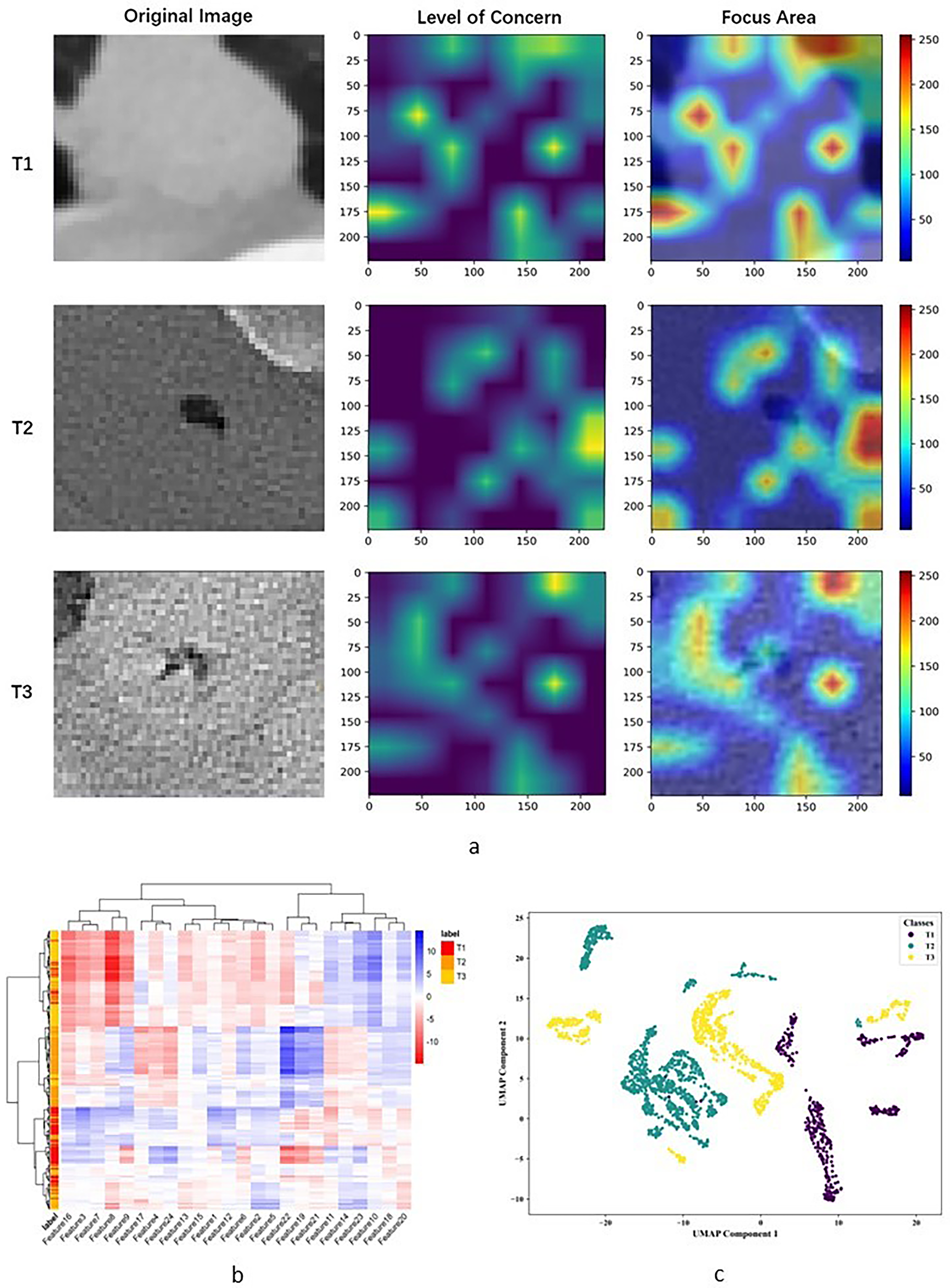
Interpretability analysis of the HMFFN in extracting DL features from CT images of esophageal cancer with different T stages. (a) Category activation map visualizing the key CT regions that the model focused on when extracting DL features. (b) Cluster heatmap generated with unsupervised hierarchical clustering of patients (vertical axis) and deep learning features expressions (i.e., the output of the last activation filters, horizontal axis). (c) Classification visualization of DL features after dimensionality reduction using the UMAP method.

Comparisons of model performance to previous studies

The comprehensive comparison with previous literatures related to tumor staging of EC was conducted. We searched PubMed (https://pubmed.ncbi.nlm.nih.gov/) for articles from January 2014 to May 2025, with the search terms (“esophageal cancer” OR “esophageal neoplasms”) AND (“model” OR “modelling”) AND “T stage” with no language restrictions, and found 794 publications. Most of the articles were basic research on genes or did not focus on the T-staging prediction of EC. The previous literature for comparison here incorporated not only T-staging diagnosis related studies (1–3), but also lymph node metastasis related research (4–6) and TNM staging related papers (7) in the field of EC because existing studies for T-staging prediction of EC using AI methods were few.^26–28^,55–58 The results (Supplementary Table 2) showed that machine learning methods were commonly adopted, and most research only used one of the clinical data, like CT, MRI, gastroscopy, or clinicopathological characteristics, relying on the single data feature without considering additive values of multi-source features in ensemble models. Besides, the sample size of the included studies was smaller than that of ours. On the whole, the highest AUC value was 0.857, and the rest were lower than 0.8, though they were basically binary classification work. Only the second article was a four-way classification study, and the ACC value was just 60.3%. The evaluation indices of the model performance reported in the first six papers all had a partial absence. No significant decline in our model performance was observed in the three-way classification task, and meanwhile, the evaluation index was more comprehensive.

Discussion

This study established and independently validated an innovative and effective T-staging diagnostic framework for EC patients before surgery. We extracted DF, RF, and CF from unstructured CT images and structured clinical variables and fused them to obtain the T-staging prediction results. The combined DL model HMFFN-AMGNN, based on the three feature types, exhibited superior and reliable predictive efficacy, yielding the highest AUC, ACC, etc.

The performance of our model improved significantly after fusing DF with CF or RF, suggesting that DF played a pivotal role in the diagnostic model. DF represents the abstract content summarized and refined by the DL model, which well supplements the information that cannot be directly collected in clinical practice or visualized by the human eye. This enhancement contributes to better overall model performance in tasks such as EC diagnosis,⁵⁹ treatment,^39,60–62 and prognosis.^40,63 Similarly, it is necessary and effective to make the best of DF for preoperative T-staging diagnosis. Wei et al. adopted CNN extracting DF from preoperative multiparametric MRI to investigate the potential value of DF in diagnosing rectal cancer T-stage and achieved an AUC of 0.854, which was significantly higher than the AUC of 0.678 and 0.747 obtained by the radiologist's assessment and clinical model, respectively (P < 0.05).⁶⁴ Liang et al. designed a multibranch aggregation network to capture and integrate tumor size, tumor shape, strongly correlated characteristics of peritumoral tissues, and spatial relationships between the tumor and surrounding invaded tissues. This approach produced a DF for nasopharyngeal carcinoma T-staging detection, yielding a mean AUC of 0.880 and outperforming conventional DL models.⁶⁵ Huang et al. reviewed DF-based T-staging methods for hollow organ cancers and concluded that DL could be a better tool for T-staging because it is more representative than radiomics features. Besides, a more refined T-staging method would be achieved by incorporating additional features related to invasion depth (e.g., RF in our study) into DL models.⁶⁶

On the methodological level of model construction, we took advantage of the combined DL model HMFFN-AMGNN for feature learning and fusion based on unstructured CT images, structured morphological data from 3D-reconstruction CT imaging, and structured clinical variables. The HMFF network primarily dealt with unstructured CT images extracting DF from small target diseased areas, while the AMGNN model mainly integrated structured data incrementally to realize multi-source feature fusion. The final results suggested that the HMFF network had the edge over the convolutional neural network (CNN) or Transformer model in processing small ROI in CT images. It simultaneously extracted local and global features of diseased regions and fused multiscale features adaptively and hierarchically, which was more conducive to the complete transfer and sufficient generalization of small target image information. The performance comparisons also proved that AMGNN, GNN integrating the meta-learning strategy and the metric learning method, can maintain superior overall prediction performance in the case of small sample sizes, and was more suitable for processing structured data in small sample scenarios than conventional machine learning methods. The adaptation of the AMGNN model to a small dataset comes from the fact that its limited parameters were all allocated to express the similarity relationship between samples. Simple network structure and low parameter settings reduced the possibility of over-fitting.^67,68

It could be calculated from the confusion matrix that among the people classified as T1-stage by the diagnostic model, the proportion of actual T1-stage patients was 86%. For the T2 and T3 stages, the corresponding proportions were 65% and 70%, respectively. The three predicted values were all superior to those of junior (T1: 77%; T2: 30%; T3: 38%) and intermediate (T1: 42%; T2: 47%; T3: 70%) clinicians. Therefore, this model demonstrates advantages in enhancing preoperative T-staging diagnosis and holds the potential to assist cardiothoracic surgeons. Interpretation of tumor T-stage is often subject to significant interobserver variability, particularly for junior or intermediate doctors at nonacademic centers.^{17,20,28,43,69} AI-assisted diagnostic strategies would provide a consistent second opinion on the T-staging of EC patients.^70,71 With the implementation of our model in clinical practice, the relative mistake diagnostic rate (i.e., predicting earlier T1 or T2 stage as more advanced T2 or T3 stage) could be reduced by approximately 2–58%, effectively avoiding more aggressive surgical approaches that led to overtreatment. Similarly, the relative omission diagnostic rate (i.e., more advanced T2 or T3 stage predicted to be earlier T1 or T2 stage) would also decrease by 1–17%, thereby minimizing undertreatment resulting from a more conservative surgery strategy.

A few studies have attempted to combine unstructured and structured medical data in analyzing tumor T-staging. Sa et al. confirmed that CT images and clinicopathological results were feasible to improve colorectal cancer T-staging prediction with an ACC from 51.04% to 86.98%. However, their imaging features were simple extractions of radiological reports by clinicians.⁴² Owing to automated and efficient DL approaches, extensive general CT features were captured for T-staging use. Zheng et al. established the Faster Region-Based CNN to make a T-staging diagnosis of gastric cancer with enhanced CT images and achieved an ACC of over 90%.²⁹ We not only utilized the HMFFN to directly extract DF from unstructured ROIs of CT images but also created the 3D reconstruction model to measure structured morphological parameters as RF from CT imaging. Besides, structured clinical baseline data, laboratory tests, and endoscopic examination results were collected to form CF, and thus these three features characterized tumor T-staging heterogeneity more comprehensively and credibly. To be specific, the utilization of multi-source features not only facilitates the extraction of potential distinct characteristics related to tumor T-stage in a multidimensional manner but also provides opportunities for mutual information supplementation and cross-validation, thereby enhancing the accuracy and reliability of prediction results. Compared to the multimodal approaches employed in T staging of other cancers,^29–32 our study also explored the integration of different algorithm functions and model architectures in DL methods for T-stage diagnosis. The core of our CAD framework lay in the introduction of the HMFF network to integrate local and global features of small-target medical images. Additionally, the AMGNN model was employed to fuse multi-source features while adapting to limited sample sizes. Therefore, the combined DL model alleviated challenges posed by the small size of EC lesions and limited labeled samples.

In view of the limited interpretability of DL models,^72,73 we aimed to explore potential biological evidence to support the model understanding of T-stage differences in CT images. The interior of T1-stage tumors and the periphery of T2-stage tumors were highlighted in the category activation heatmap, whereas the focus for T3-stage tumors was scattered and lacked highly recognizable regions. From a biological perspective of UMAP representations, we infer that sub-clusters within the T1 stage correspond to tumors with high intra-tumor heterogeneity. In contrast, sub-clusters in the T2 stage indicate tumors with high heterogeneity characteristics in the periphery. However, these changes appear particularly extensive and are common in tumors at the T3-stage. Some subclusters exhibited severe internal tumor changes, while others showed signs of external invasion. The DL model tended to misclassify T3-stage images as T1 or T2 stage, aligning with the lowest ACC in the confusion matrix. The changes in internal and external tumor cells or stroma may reflect the heterogeneity of the tumor microenvironment across these stages. Lin et al. mentioned that the tumor microenvironment in EC changes with different tumor stages.⁷⁴ Specifically, Jiang et al. confirmed that the increase in M1 macrophages was negatively correlated with the T stage of EC (P < 0.05),⁷⁵ whereas Wang et al. discovered that the ratio of neutrophils to lymphocytes around the tumor had a strong positive correlation with the T stage of EC (P < 0.001).⁷⁶ Li et al. suggested that the activation and infiltration extent of interstitial cells in EC patients were also positively correlated with the T stage (P < 0.05).⁷⁷ Nevertheless, more exact experimental and bioinformatics evidence is required from future fundamental research to determine the detailed information on tumors and tumor microenvironments corresponding to abstract DF that represent the T-stage differences.

This study had some limitations. First, the research sample may not fully represent the target clinical population. Most patients in the multicenter dataset were from the southwest region of China and patients with stage T4 were excluded. It may limit the model's ability to assist clinicians in determining appropriate surgical strategies for individuals from other ethnic backgrounds and those with distinct disease subtypes. We plan to extend this model to national and international multicenter studies to validate its generalizability and clinical applicability. Second, the modeling pipeline depends on manual image segmentation, introducing potential variability that could bias manually extracted morphological features and restrict the diversity of deep features learned by the model. Thus, future research should focus on optimizing feasible learning algorithms and refining the feature extraction framework by leveraging advanced unsupervised models.

Conclusion

In conclusion, we established a preoperative T-stage prediction framework for EC centered on the combined DL model HMFFN-AMGNN. It utilized CT features and clinical variables to improve diagnostic accuracy and reliability. To our knowledge, this study is the first to investigate the capacity of multiple features from unstructured CT images and structured clinical data to differentiate between tumor T stages. Evaluation experiments using multicenter datasets verified the effectiveness, robustness, and superiority of the proposed diagnostic method. This CAD tool was developed to facilitate clinical decision-making and optimize individualized therapeutic strategies.

Supplemental Material

sj-docx-1-dhj-10.1177_20552076261427129 - Supplemental material for The combined deep learning model integrating CT features and clinical variables for preoperative T-stage diagnosis in esophageal cancer: A multicenter study

Supplemental material, sj-docx-1-dhj-10.1177_20552076261427129 for The combined deep learning model integrating CT features and clinical variables for preoperative T-stage diagnosis in esophageal cancer: A multicenter study by Li Qian, Pengyu Wang, Jincheng Chen, Xicheng Chen, Ling Zhang, Ning Tang, Jiarui Li, Zhen Huang, Ping He, Wei Wu and Yazhou Wu in DIGITAL HEALTH

Characteristic	Internal dataset (Institution 1, n = 394)	External dataset (Institutions 2 and 3, n = 49)	P-value
Age, mean (SD), year	61.95 (7.64)	61.68 (7.00)	61.82 (7.77)	62.47 (6.72)	63.76 (7.18)	60.43 (9.28)	60.47 (5.56)	62.24 (6.39)	64.21 (8.74)	61.67 (8.98)	63.53 (7.45)	62.95 (7.16)	0.577
Gender, n (%)	66 (100.00)	108 (100.00)	89 (100.00)	19 (100.00)	25 (100.00)	21 (100.00)	17 (100.00)	25 (100.00)	24 (100.00)	12 (100.00)	17 (100.00)	20 (100.00)	0.294
Male, n (%)	50 (76.76)	86 (79.63)	71 (79.78)	14 (73.68)	22 (88.00)	19 (90.48)	12 (70.59)	24 (96.00)	22 (91.67)	10 (83.33)	15 (88.24)	16 (80.00)
Female, n (%)	16 (24.24)	22 (20.47)	18 (20.22)	5 (26.32)	3 (12.00)	2 (9.52)	5 (29.41)	1 (4.00)	2 (8.33)	2 (16.67)	2 (11.76)	4 (20.00)
BMI, mean (SD)	22.77 (2.88)	23.17 (2.89)	22.81 (3.26)	23.83 (2.29)	22.76 (1.50)	21.92 (3.14)	23.90 (4.58)	21.23 (2.06)	22.42 (2.59)	23.83 (3.21)	22.70 (3.40)	24.15 (3.97)	0.191
TNM stage, n (%)	66 (100.00)	108 (100.00)	89 (100.00)	19 (100.00)	25 (100.00)	21 (100.00)	17 (100.00)	25 (100.00)	24 (100.00)	12 (100.00)	17 (100.00)	20 (100.00)	0.082
Ⅰ, n (%)	59 (89.39)	10 (9.26)	0 (0.00)	16 (84.21)	3 (12.00)	0 (0.00)	16 (94.12)	0 (0.00)	0 (0.00)	8 (66.67)	3 (17.65)	0 (0.00)
Ⅱ, n (%)	6 (9.09)	68 (62.96)	58 (65.17)	3 (15.79)	17 (68.00)	12 (57.14)	1 (5.88)	15 (60.00)	15 (62.50)	2 (16.67)	7 (41.18)	7 (35.00)
Ⅲ, n (%)	1 (1.52)	29 (26.50)	26 (29.21)	0 (0.00)	4 (16.00)	8 (38.10)	0 (0.00)	10 (40.00)	9 (37.50)	0 (0.00)	6 (35.29)	11 (55.00)
Ⅳ, n (%)	0 (0.00)	1 (0.93)	5 (5.62)	0 (0.00)	1 (4.00)	1 (4.76)	0 (0.00)	0 (0.00)	0 (0.00)	2 (16.67)	1 (5.88)	2 (10.00)
Histology, n (%)	66 (100.00)	108 (100.00)	89 (100.00)	19 (100.00)	25 (100.00)	21 (100.00)	17 (100.00)	25 (100.00)	24 (100.00)	12 (100.00)	17 (100.00)	20 (100.00)	0.362
SCC, n (%)	65 (98.48)	105 (97.22)	88 (98.88)	18 (94.74)	25 (100.00)	20 (95.24)	15 (88.24)	25 (100.00)	23 (95.83)	12 (100.00)	17 (100.00)	20 (100.00)
Non-SCC, n (%)	1 (1.52)	3 (2.78)	1 (1.12)	1 (5.26)	0 (0.00)	1 (4.76)	2 (11.76)	0 (0.00)	1 (4.17)	0 (0.00)	0 (0.00)	0 (0.00)
Tumor location under gastroscopy, n (%)	66 (100.00)	108 (100.00)	89 (100.00)	19 (100.00)	25 (100.00)	21 (100.00)	17 (100.00)	25 (100.00)	24 (100.00)	12 (100.00)	17 (100.00)	20 (100.00)	0.955
Upper segment, n (%)	7 (10.61)	8 (7.41)	12 (13.48)	2 (10.53)	1 (4.00)	2 (9.52)	2 (11.76)	0 (0.00)	2 (8.33)	1 (8.33)	1 (5.88)	2 (10.00)
Middle and upper segment, n (%)	4 (6.06)	13 (12.04)	6 (6.74)	0 (0.00)	1 (4.00)	3 (14.29)	2 (11.76)	1 (0.04)	3 (0.125)	1 (8.33)	1 (5.88)	3 (15.00)
Middle segment, n (%)	30 (45.45)	35 (32.41)	26 (29.21)	10 (52.63)	13 (52.00)	5 (23.81)	8 (47.06)	9 (0.36)	11 (45.83)	4 (33.33)	8 (47.06)	7 (35.00)
Middle and lower segment, n (%)	9 (13.64)	21 (19.44)	16 (17.98)	1 (5.26)	4 (16.00)	4 (19.05)	3 (17.65)	6 (0.24)	3 (0.125)	4 (33.33)	3 (17.65)	3 (15.00)
Lower segment, n (%)	16 (24.24)	31 (28.70)	29 (32.58)	6 (31.58)	6 (24.00)	7 (33.33)	2 (11.76)	9 (0.36)	5 (20.83)	2 (16.67)	4 (23.53)	5 (25.00)
Smoking status, n (%)	66 (100.00)	108 (100.00)	89 (100.00)	19 (100.00)	25 (100.00)	21 (100.00)	17 (100.00)	25 (100.00)	24 (100.00)	12 (100.00)	17 (100.00)	20 (100.00)	0.272
Former, n (%)	40 (60.61)	68 (62.96)	59 (66.29)	11 (57.89)	18 (72.00)	13 (61.90)	8 (47.06)	22 (88.00)	18 (75.00)	8 (66.67)	10 (58.82)	10 (50.00)
Never, n (%)	26 (39.39)	40 (37.04)	30 (33.71)	8 (42.11)	7 (28.00)	8 (38.10)	9 (52.94)	3 (12.00)	6 (25.00)	4 (33.33)	7 (41.18)	10 (50.00)
Drinking status, n (%)	66 (100.00)	108 (100.00)	89 (100.00)	19 (100.00)	25 (100.00)	21 (100.00)	17 (100.00)	25 (100.00)	24 (100.00)	12 (100.00)	17 (100.00)	20 (100.00)	0.313
Former, n (%)	38 (57.58)	68 (62.96)	60 (67.42)	11 (57.89)	14 (56.00)	13 (61.90)	7 (41.18)	20 (80.00)	17 (70.83)	3 (25.00)	11 (64.71)	10 (50.00)
Never, n (%)	28 (42.42)	40 (37.04)	29 (32.58)	8 (42.11)	11 (44.00)	8 (38.10)	10 (58.82)	5 (20.00)	7 (29.17)	9 (75.00)	6 (35.29)	10 (50.00)

Data characteristics	AUC (95% CI)	Accuracy (95% CI)	Precision (95% CI)	Recall (95% CI)	F1-score (95% CI)
DF	0.787 (0.721–0.852)	60.606 (50.000–72.727)	62.673 (51.634–73.765)	60.185 (48.350–72.258)	61.406 (48.627–71.605)
RF	0.774 (0.696–0.844)	71.212 (60.606–81.818)	49.487 (42.708–55.607)	56.066 (49.376–61.875)	51.759 (44.708–57.621)
CF	0.716 (0.633–0.794)	59.091 (46.970–71.212)	43.160 (35.000–50.556)	54.895 (47.874–61.209)	46.712 (38.840–53.333)
DF + RF	0.800 (0.731–0.860)	62.121 (50.000–72.727)	54.215 (37.771–78.413)	53.694 (45.040–63.154)	50.148 (40.256–61.396)
DF + CF	0.785 (0.715–0.852)	65.152 (53.030–75.758)	68.950 (56.734–80.139)	67.210 (57.729–76.389)	63.933 (51.499–74.680)
RF + CF	0.776 (0.704–0.844)	66.667 (54.545–77.273)	46.090 (38.636–53.301)	52.533 (45.086–59.249)	48.340 (40.507–54.988)
DF + RF + CF	0.848 (0.788–0.902)	72.727 (62.121–83.333)	72.839 (59.911–84.803)	69.559 (58.782–80.159)	69.665 (57.361–80.317)

Data characteristics	AUC (95% CI)	Accuracy (95% CI)	Precision (95% CI)	Recall (95% CI)	F1-score (95% CI)
DF	0.742 (0.644–0.828)	63.265 (48.980–75.510)	39.591 (30.476–48.810)	48.659 (37.582–58.774)	43.193 (33.048–52.125)
RF	0.802 (0.723–0.876)	69.388 (57.143–81.633)	46.825 (38.492–55.159)	59.649 (52.747–65.217)	52.199 (44.806–58.602)
CF	0.681 (0.583–0.778)	61.224 (46.939–73.469)	73.704 (32.222–81.878)	52.337 (40.000–63.248)	50.271 (35.973–63.313)
DF + RF	0.794 (0.703–0.877)	71.429 (59.184–83.673)	65.236 (51.410–80.152)	65.369 (51.157–80.471)	65.243 (50.859–79.199)
DF + CF	0.756 (0.661–0.842)	67.347 (55.102–79.592)	73.333 (62.654–84.188)	65.377 (51.323–78.430)	65.043 (49.750–77.914)
RF + CF	0.709 (0.607–0.798)	65.306 (51.020–77.551)	44.841 (36.201–53.125)	56.000 (49.425–61.905)	47.893 (38.760–55.295)
DF + RF + CF	0.867 (0.792–0.929)	77.551 (65.306–87.755)	77.908 (66.071–89.019)	77.895 (65.765–89.072)	77.731 (65.074–88.333)

Methods	AUC (95% CI)	Accuracy (95% CI)	Precision (95% CI)	Recall (95% CI)	F1-score (95% CI)
ConvNeXt-T	0.600 (0.515–0.683)	40.000 (27.692–52.308)	29.894 (10.256–49.180)	35.294 (33.333–39.583)	22.448 (15.447–30.527)
Resnet-34	0.606 (0.525–0.690)	44.615 (32.308–56.923)	45.723 (31.588–59.957)	43.311 (30.982–55.693)	43.442 (30.334–55.342)
EfficientNet-B0	0.638 (0.559–0.716)	43.077 (30.769–55.385)	48.201 (34.066–61.430)	42.142 (29.789–54.020)	43.361 (30.166–55.300)
Swin transformer-T	0.613 (0.534–0.694)	43.077 (30.769–55.385)	47.778 (26.796–64.141)	40.955 (29.499–52.778)	39.646 (26.299–52.433)
T2T-ViT_t-24	0.638 (0.563–0.718)	40.000 (27.692–52.308)	46.061 (21.494–69.444)	36.781 (27.895–46.019)	31.353 (19.337–43.111)
HMFFN-AMGNN (DF)	0.787 (0.721–0.852)	60.606 (50.000–72.727)	62.673 (51.634–73.765)	60.185 (48.350–72.258)	61.406 (48.627–71.605)
HMFFN-AMGNN (DF + RF + CF)	0.848 (0.788–0.902)	72.727 (62.121–83.333)	72.839 (59.911–84.803)	69.559 (58.782–80.159)	69.665 (57.361–80.317)

Methods	AUC (95% CI)	Accuracy (95% CI)	Precision (95% CI)	Recall (95% CI)	F1-score (95% CI)
Support vector machine	0.680 (0.602–0.755)	41.791 (29.851–55.224)	40.980 (27.408–55.662)	39.970 (28.932–51.346)	38.462 (26.607–50.831)
Logistic regression	0.677 (0.601–0.753)	43.284 (31.343–55.224)	41.852 (30.263–53.947)	43.727 (32.660–55.525)	42.445 (31.028–53.326)
K-nearest neighbor	0.701 (0.630–0.771)	49.254 (37.313–61.194)	50.397 (37.947–63.145)	49.364 (37.065–61.648)	49.781 (37.155–61.306)
Naïve Bayes	0.709 (0.634–0.782)	49.254 (37.313–61.194)	47.196 (34.454–60.804)	50.121 (40.058–60.790)	46.514 (34.964–58.052)
Random forest	0.739 (0.668–0.806)	53.731 (41.791–65.672)	54.095 (42.271–65.523)	53.727 (42.320–65.870)	53.890 (41.857–64.665)
Multilayer perceptron	0.708 (0.631–0.783)	46.269 (34.328–58.209)	44.433 (31.159–58.283)	47.758 (36.928–58.394)	43.495 (32.305–54.219)
HMFFN-AMGNN (RF + CF)	0.776 (0.704–0.844)	66.667 (54.545–77.273)	46.090 (38.636–53.301)	52.533 (45.086–59.249)	48.340 (40.507–54.988)
HMFFN-AMGNN (DF + RF + CF)	0.848 (0.788–0.902)	72.727 (62.121–83.333)	72.839 (59.911–84.803)	69.559 (58.782–80.159)	69.665 (57.361–80.317)

Approaches	AUC (95% CI)	ACC (%) (95% CI)	PRE (%) (95% CI)	SEN (%) (95% CI)	F1-score (%) (95% CI)
Junior clinician	0.580 (0.524–0.636)	44.000 (34.000–54.000)	52.237 (41.946–62.192)	43.995 (34.722–53.724)	44.017 (33.895–53.245)
Intermediate clinician	0.625 (0.567–0.681)	50.000 (40.000–60.000)	53.078 (42.801–63.019)	50.267 (40.196–60.664)	49.601 (39.188–59.517)
Senior clinician	0.685 (0.630–0.744)	58.000 (49.000–68.000)	71.117 (37.643–77.528)	62.981 (57.544–68.468)	51.215 (43.438–59.423)
Our proposed model	0.848 (0.788–0.902)	72.727 (62.121–83.333)	72.839 (59.911–84.803)	69.559 (58.782–80.159)	69.665 (57.361–80.317)

Footnotes

Abbreviations

The following abbreviations are used in this manuscript:

Acknowledgments

The code for the constructed model needs to be thanked @article{huo2022hifuse, title={HiFuse: Hierarchical Multi-Scale Feature Fusion Network for Medical Image Classification}, author={Huo, Xiangzuo and Sun, Gang and Tian, Shengwei and Wang, Yan and Yu, Long and Long, Jun and Zhang, Wendong and Li, Aolun}, journal={arXiv preprint arXiv:2209.10218}, year={2022}} and @journal{song2021jbhi, title={Auto-Metric Graph Neural Network Based on a Meta-learning Strategy for the Diagnosis of Alzheimer's disease}, author={Xiaofan Song, Mingyi Mao and Xiaohua Qian}, journal={IEEE Journal of Biomedical and Health Informatics}, month = {January}, year={2021}}.

ORCID iDs

Li Qian

Pengyu Wang

Jincheng Chen

Ping He

Yazhou Wu

Ethical approval

The study was conducted in accordance with the Declaration of Helsinki, and approved by the Ethics Committee of Southwest Hospital (Protocol Code KY2021165). The need to obtain written informed consent from the patients was waived because the data used for research analysis had been anonymized by removing personal information.

Contributorship

Conceptualization: Li Qian, Ning Tang, and Yazhou Wu; data curation: Li Qian, Pengyu Wang, Jincheng Chen, and Zhen Huang; formal analysis: Li Qian, Pengyu Wang, Jincheng Chen, and Xicheng Chen; funding acquisition: Yazhou Wu; Investigation, Li Qian, Jincheng Chen, and Ling Zhang; methodology: Li Qian, Ning Tang, and Yazhou Wu; project administration: Ping He, Wei Wu, and Yazhou Wu; resources: Jincheng Chen, Ping He, and Wei Wu; software: Li Qian, Jincheng Chen, and Jiarui Li; supervision: Ping He, Wei Wu, and Yazhou Wu; validation: Li Qian, Pengyu Wang, Ping He, and Yazhou Wu; visualization: Li Qian, Pengyu Wang, and Jiarui Li; writing – original draft: Li Qian and Xicheng Chen; writing – review and editing: Pengyu Wang, Xicheng Chen, Ling Zhang, Zhen Huang, and Yazhou Wu.

Funding

The authors disclosed receipt of the following financial support for the research, authorship, and/or publication of this article: This work was supported by the National Natural Science Foundation of China (Grant Numbers 81872716, 82173621, 82574207).

Declaration of conflicting interests

The authors declared no potential conflicts of interest with respect to the research, authorship, and/or publication of this article.

Data availability statement

CT images and clinical data of esophageal cancer patients reported in this paper will be shared by the lead contact upon request. All original code has been deposited at github and is publicly available as of the date of publication. This has also been listed in the key resources table. Any additional information required to reanalyze the data reported in this paper is available from the lead contact upon reasonable request.

Guarantor

Yazhou Wu, the corresponding author, serves as the guarantor of this work.

Supplemental material

Supplemental material for this article is available online.

References

Bien

Nguyen

TH-A

Aljehani

, et al. Changing epidemiology of esophageal cancer: A population-based study over 43 years (1975–2018). J Clin Oncol 40. Epub ahead of print 1 February 2022. DOI: 10.1200/JCO.2022.40.4_suppl.247.

Sung

Ferlay

Siegel

, et al. Global cancer statistics 2020: GLOBOCAN estimates of incidence and mortality worldwide for 36 cancers in 185 countries. CA Cancer J Clin 2021; 71: 209–249.

Morgan

Soerjomataram

Rumgay

, et al. The global landscape of esophageal squamous cell carcinoma and esophageal adenocarcinoma incidence and mortality in 2020 and projections to 2040: new estimates from GLOBOCAN 2020. Gastroenterology 2022; 163: 649–658.e2.

Chen

Zheng

Zhang

, et al. Patterns and trends in esophageal cancer incidence and mortality in China: an analysis based on cancer registry data. J Natl Cancer Center 2023; 3: 21–27.

Yang

Lin

, et al. Burden, trends, and risk factors of esophageal cancer in China from 1990 to 2017: an up-to-date overview and comparison with those in Japan and South Korea. J Hematol Oncol 2020; 13: 146.

Zhu

Wang

Deng

, et al. Epidemiological landscape of esophageal cancer in Asia: results from GLOBOCAN 2020. Thorac Cancer 2023; 14: 992–1003.

, et al. The disease and economic burdens of esophageal cancer in China from 2013 to 2030: dynamic cohort modeling study. JMIR Public Health Surveill 2022; 8: e33191.

Chen

Man

, et al. Changing trends in the disease burden of esophageal cancer in China from 1990 to 2017 and its predicted level in 25 years. Cancer Med 2021; 10: 1889–1899.

Zheng

, et al. Esophageal cancer: epidemiology, risk factors and screening. Chin J Cancer Res 2021; 33: 535–547.

10.

Allemani

Matsuda

Di Carlo

, et al. Global surveillance of trends in cancer survival 2000–14 (CONCORD-3): analysis of individual records for 37 513 025 patients diagnosed with one of 18 cancers from 322 population-based registries in 71 countries. Lancet 2018; 391: 1023–1075.

11.

Ajani

D’Amico

Bentrem

, et al. Esophageal and esophagogastric junction cancers, version 2.2023, NCCN clinical practice guidelines in oncology. J Natl Compr Canc Netw 2023; 21: 393–422.

12.

Shapiro

van Lanschot

JJB

Hulshof

MCCM

, et al. Neoadjuvant chemoradiotherapy plus surgery versus surgery alone for oesophageal or junctional cancer (CROSS): long-term results of a randomised controlled trial. Lancet Oncol 2015; 16: 1090–1098.

13.

Mariette

Dahan

Mornex

, et al. Surgery alone versus chemoradiotherapy followed by surgery for stage I and II esophageal cancer: final analysis of randomized controlled phase III trial FFCD 9901. J Clin Oncol 2014; 32: 2416–U201.

14.

Obermannova

Alsina

Cervantes

, et al. Oesophageal cancer: ESMO clinical practice guideline for diagnosis, treatment and follow-up. Ann Oncol 2022; 33: 992–1004.

15.

Yang

Liu

Chen

, et al. Neoadjuvant chemoradiotherapy followed by surgery versus surgery alone for locally advanced squamous cell carcinoma of the esophagus (NEOCRTEC5010): a phase III multicenter, randomized, open-label clinical trial. JCO 2018; 36: 2796–2803.

16.

Hou

Zhou

Sun

. Deep-learning-based 3D super-resolution MRI radiomics model: superior predictive performance in preoperative T-staging of rectal cancer. Eur Radiol 2023; 33: 1–10.

17.

Cheng

Liu

, et al. Evaluation of optimal monoenergetic images acquired by dual-energy CT in the diagnosis of T staging of thoracic esophageal cancer. Insights Imaging 2023; 14: 33.

18.

Wang

Zhang

, et al.

Could tumour volume and major and minor axis based on CTA statistical anatomy improve the pre-operative T-stage in oesophageal cancer?

Cancer Med 2023; 12: 14037–14051.

19.

Lee

Hoseok

Kim

S-J

, et al. Clinical implication of PET/MR imaging in preoperative esophageal cancer staging: comparison with PET/CT, endoscopic ultrasonography, and CT. J Nucl Med 2014; 55: 1242–1247.

20.

Guo

Wang

Qin

, et al. A prospective analysis of the diagnostic accuracy of 3T MRI, CT and endoscopic ultrasound for preoperative T staging of potentially resectable esophageal cancer. Cancer Imaging 2020; 20: 64.

21.

Ringe

Meyer

Ringe

, et al. Value of oral effervescent powder administration for multidetector CT evaluation of esophageal cancer. Eur J Radiol 2015; 84: 215–220.

22.

Winiker

Mantziari

Figueiredo

, et al. Accuracy of preoperative staging for a priori resectable esophageal cancer. Dis Esophagus 2018; 31: 1–6.

23.

Jiang

Zhang

, et al. Human-recognizable CT image features of subsolid lung nodules associated with diagnosis and classification by convolutional neural networks. Eur Radiol 2021; 31: 7303–7315.

24.

Zhu

Liu

Gao

, et al. Explainable classification of benign-malignant pulmonary nodules with neural networks and information bottleneck. IEEE Trans Neural Networks Learning Systems 2025; 36: 2028–2039.

25.

Wang

Zheng

, et al. Development of an AI system for accurately diagnose hepatocellular carcinoma from computed tomography imaging data. Br J Cancer 2021; 125: 1111–1121.

26.

Yang

, et al. Computed tomography-based radiomics in predicting T stage and length of esophageal squamous cell carcinoma. Front Oncol 2021; 11: 722961.

27.

Wang

Huang

Zhao

, et al.

Esophageal wall thickness on CT scans: can it predict the T stage of primary thoracic esophageal squamous cell carcinoma?

Esophagus 2022; 19: 269–277.

28.

Wei

Chen

, et al. The T stage of esophageal cancer can be effectively predicted by muscularis propria thickness and muscularis propria + mucosa thickness under ultrasonic gastroscopy. Thorac Cancer 2023; 14: 127–134.

29.

Zheng

Zhang

, et al. Establishment and applicability of a diagnostic system for advanced gastric cancer T staging based on a faster region-based convolutional neural network. Front Oncol 2020; 10: 1238.

30.

Tian

, et al. Deep learning models for preoperative T-stage assessment in rectal cancer using MRI: exploring the impact of rectal filling. Front Med 2023; 10: 1326324.

31.

Yang

Guo

, et al. Automatic T staging using weakly supervised deep learning for nasopharyngeal carcinoma on MR images. J Magn Reson Imaging 2020; 52: 1074–1082.

32.

Gao

Ying

, et al. A novel preoperative prediction model based on deep learning to predict neoplasm T staging and grading in patients with upper tract urothelial carcinoma. J Clin Med 2022; 11: 5815.

33.

Wang

Hong

Q-Q

, et al. Transfer learning for medical images analyses: a survey. Neurocomputing 2022; 489: 230–254.

34.

Zhou

L-Q

Zeng

S-E

J-W

, et al. Deep learning predicts cervical lymph node metastasis in clinically node-negative papillary thyroid carcinoma. Insights Imaging 2023; 14: 222.

35.

Sun

Wang

, et al. Radiomic features of pretreatment MRI could identify T stage in patients with rectal cancer: preliminary findings. J Magn Reson Imaging 2018; 48: 615–621.

36.

Tang

Zhang

Wei

, et al. Improving the performance of lung nodule classification by fusing structured and unstructured data. Inf Fusion 2022; 88: 161–174.

37.

Jiao

Xiao

, et al. Integration of deep learning radiomics and counts of circulating tumor cells improves prediction of outcomes of early stage NSCLC patients treated with stereotactic body radiation therapy. Int J Radiat Oncol Biol Phys 2022; 112: 1045–1054.

38.

Xia

Chen

, et al. Development and validation of a deep learning signature for predicting lymph node metastasis in lung adenocarcinoma: comparison with radiomics signature and clinical-semantic model. Eur Radiol 2023; 33: 1949–1962.

39.

Xie

Yang

, et al. Computed tomography-based deep-learning prediction of neoadjuvant chemoradiotherapy treatment response in esophageal squamous cell carcinoma. Radiother Oncol 2021; 154: 6–13.

40.

Cui

Dong

, et al. Integrating clinical data and attentional CT imaging features for esophageal Fistula prediction in esophageal cancer. Front Oncol 2021; 11: 688706.

41.

Ding

Cui

, et al. Integrating preoperative computed tomography and clinical factors for lymph node metastasis prediction in esophageal squamous cell carcinoma by feature-wise attentional graph neural network. Int J Radiat Oncol Biol Phys 0. Epub ahead of print 11 January 2023. DOI: 10.1016/j.ijrobp.2022.12.050

42.

, et al. Development and validation of a preoperative prediction model for colorectal cancer T-staging based on MDCT images and clinical information. Oncotarget 2017; 8: 55308–55318.

43.

Haefliger

Jreige

Du Pasquier

, et al. Esophageal cancer T-staging on MRI: a preliminary study using cine and static MR sequences. Eur J Radiol 2023; 166: 111001.

44.

Huo

Sun

Tian

, et al. Hifuse: hierarchical multi-scale feature fusion network for medical image classification. Biomed Signal Process Control 2024; 87: 105534.

45.

Song

Mao

Qian

. Auto-Metric graph neural network based on a meta-learning strategy for the diagnosis of Alzheimer’s disease. IEEE J Biomed Health Inform 2021; 25: 3141–3152.

46.

Cotsoglou

Granieri

Bassetto

, et al. Dynamic surgical anatomy using 3D reconstruction technology in complex hepato-biliary surgery with vascular involvement. Results from an international multicentric survey. HPB (Oxford) 2024; 26: 83–90.

47.

Ahmed

Ali

Abdelhakam

, et al. Detection of hepatocellular carcinoma feeding vessels: MDCT angiography with 3D reconstruction versus digital subtraction angiography. BMC Med Imag 2024; 24: 250.

48.

Weber

Sarich

PEA

Vaneckova

, et al. Cancer incidence and cancer death in relation to tobacco smoking in a population-based Australian cohort study. Intl Journal of Cancer 2021; 149: 1076–1088.

49.

Chen

Z-M

Peto

Iona

, et al. Emerging tobacco-related cancer risks in China: a nationwide, prospective study of 0.5 million adults. Cancer 2015; 121: 3097–3106.

50.

Sha

Wang

. Relationship between alcohol consumption and the risks of liver cancer, esophageal cancer, and gastric cancer in China: meta-analysis based on case-control studies. Medicine (Baltimore) 2021; 100: e26982.

51.

Tian

Zuo

Liu

, et al. Cumulative evidence for the relationship between body mass index and the risk of esophageal cancer: an updated meta-analysis with evidence from 25 observational studies. J Gastroenterol Hepatol 2020; 35: 730–743.

52.

Siegel

Miller

Jemal

. Cancer statistics, 2019. CA Cancer J Clin 2019; 69: 7–34.

53.

Hsu

P-K

Chien

L-I

Huang

C-S

, et al. Treatment patterns and outcomes in patients with esophageal cancer: an analysis of a multidisciplinary tumor board database. Ann Surg Oncol 2022; 29: 572–585.

54.

Sanikini

Muller

Sophiea

, et al. Anthropometric and reproductive factors and risk of esophageal and gastric cancer by subtype and subsite: results from the European prospective investigation into cancer and nutrition (EPIC) cohort. Int J Cancer 2020; 146: 929–942.

55.

Zhang

Yan

, et al. Machine learning models predict lymph node metastasis in patients with stage T1-T2 esophageal squamous cell carcinoma. Front Oncol 2022; 12: 986358.

56.

Shen

Liu

Wang

, et al. Building CT radiomics based nomogram for preoperative esophageal cancer patients lymph node metastasis prediction. Transl Oncol 2018; 11: 815–824.

57.

Shen

Qin

, et al. The MR radiomic signature can predict preoperative lymph node metastasis in patients with esophageal cancer. Eur Radiol 2019; 29: 906–914.

58.

Wang

Tan

, et al. Radiomics approach for preoperative identification of stages I-II and III-IV of esophageal cancer. Chin J Cancer Res 2018; 30: 396-+.

59.

Gong

Bang

Jung

, et al. Deep-Learning for the diagnosis of esophageal cancers and precursor lesions in endoscopic images: a model establishment and nationwide multicenter performance verification study. J Pers Med 2022; 12: 1052.

60.

Draguet

Barragán-Montero

Vera

, et al. Automated clinical decision support system with deep learning dose prediction and NTCP models to evaluate treatment complications in patients with esophageal cancer. Radiother Oncol 2022; 176: 101–107.

61.

Liu

Men

, et al. A deep learning classifier based on Pre-radiation computed tomography and clinical parameters to predict pathological complete response after neoadjuvant chemoradiation in esophageal cancer. Int J Radiat Oncol Biol Phys 2022; 114: E163–E163.

62.

Zhu

Jin

, et al. Deep learning based lymph node gross tumor volume detection via distance-guided gating using CT and 18F-FDG PET in esophageal cancer radiotherapy. Int J Radiat Oncol Biol Phys 2021; 111: E87–E88.

63.

Gong

Zhang

Huang

, et al. CT-Based Deep learning model for predicting local recurrence-free survival in esophageal squamous cell carcinoma patients received concurrent chemo-radiotherapy: a multicenter study. Int J Radiat Oncol Biol Phys 2022; 114: S121–S122.

64.

Wei

Wang

Chen

, et al. Deep learning-based multiparametric MRI model for preoperative T-stage in rectal cancer. J Magn Reson Imaging 2024; 59: 1083–1092.

65.

Liang

Dong

Yang

, et al. A multi-perspective information aggregation network for automated T-staging detection of nasopharyngeal carcinoma. Phys Med Biol 2022; 67: 245007.

66.

Huang

, et al. Radiomics-based T-staging of hollow organ cancers. Front Oncol 2023; 13: 1191519.

67.

Torres

LHM

Ribeiro

Arrais

. Few-shot learning with transformers via graph embeddings for molecular property prediction. Expert Syst Appl 2023; 225: 120005.

68.

Chen

Wei

, et al. Hierarchical graph neural networks for few-shot learning. IEEE Trans Circuits Syst Video Technol 2022; 32: 240–252.

69.

Wang

Zhu

, et al. Impact of endoscopic ultrasonography on the accuracy of T staging in esophageal cancer and factors associated with its accuracy: a retrospective study. Medicine (Baltimore) 2022; 101: e28603.

70.

Wang

, et al. Segmentation prompts classification: a nnUNet-based 3D transfer learning framework with ROI tokenization and cross-task attention for esophageal cancer T-stage diagnosis. Expert Syst Appl 2024; 258: 125067.

71.

Zhang

Chen

Wang

Z-Z

, et al. Esophagogastroscopy for predicting endoscopic ultrasonography T-stage by utilizing deep learning methods in esophageal cancer. Appl Intell 2024; 54: 9286–9294.

72.

Patricio

Neves

Lincs

, et al. Explainable deep learning methods in medical image classification: a survey. ACM Comput Surv 2024; 56: 85.

73.

Zhang

, et al. Deep learning with radiomics for disease diagnosis and treatment: challenges and potential. Front Oncol 2022; 12: 773840.

74.

Lin

Karakasheva

Hicks

, et al. The tumor microenvironment in esophageal cancer. Oncogene 2016; 35: 5337–5349.

75.

Jiang

Liang

, et al. Distribution and prognostic impact of M1 macrophage on esophageal squamous cell carcinoma. Carcinogenesis 2021; 42: 537–545.

76.

Wang

Jia

Wang

, et al. The clinical significance of tumor-infiltrating neutrophils and neutrophil-to-CD8 + lymphocyte ratio in patients with resectable esophageal squamous cell carcinoma. J Transl Med 2014; 12: 7.

77.

Zeng

Jiang

, et al. Stromal microenvironment promoted infiltration in esophageal adenocarcinoma and squamous cell carcinoma: a multi-cohort gene-based analysis. Sci Rep 2020; 10: 18589.

Supplementary Material

Please find the following supplemental material available below.

For Open Access articles published under a Creative Commons License, all supplemental material carries the same license as the article it is associated with.

For non-Open Access articles published, all supplemental material carries a non-exclusive license, and permission requests for re-use of supplemental material or any part of supplemental material shall be sent directly to the copyright owner as specified in the copyright notice associated with the article.

0.00 MB

1.76 MB

Characteristic	Internal dataset (Institution 1, n = 394)									External dataset (Institutions 2 and 3, n = 49)			P-value
	Train cohort (n = 263)			Validation cohort (n = 65)			Test cohort (n = 66)			Test cohort (n = 49)
	T1	T2	T3	T1	T2	T3	T1	T2	T3	T1	T2	T3
Age, mean (SD), year	61.95 (7.64)	61.68 (7.00)	61.82 (7.77)	62.47 (6.72)	63.76 (7.18)	60.43 (9.28)	60.47 (5.56)	62.24 (6.39)	64.21 (8.74)	61.67 (8.98)	63.53 (7.45)	62.95 (7.16)	0.577
Gender, n (%)	66 (100.00)	108 (100.00)	89 (100.00)	19 (100.00)	25 (100.00)	21 (100.00)	17 (100.00)	25 (100.00)	24 (100.00)	12 (100.00)	17 (100.00)	20 (100.00)	0.294
Male, n (%)	50 (76.76)	86 (79.63)	71 (79.78)	14 (73.68)	22 (88.00)	19 (90.48)	12 (70.59)	24 (96.00)	22 (91.67)	10 (83.33)	15 (88.24)	16 (80.00)
Female, n (%)	16 (24.24)	22 (20.47)	18 (20.22)	5 (26.32)	3 (12.00)	2 (9.52)	5 (29.41)	1 (4.00)	2 (8.33)	2 (16.67)	2 (11.76)	4 (20.00)
BMI, mean (SD)	22.77 (2.88)	23.17 (2.89)	22.81 (3.26)	23.83 (2.29)	22.76 (1.50)	21.92 (3.14)	23.90 (4.58)	21.23 (2.06)	22.42 (2.59)	23.83 (3.21)	22.70 (3.40)	24.15 (3.97)	0.191
TNM stage, n (%)	66 (100.00)	108 (100.00)	89 (100.00)	19 (100.00)	25 (100.00)	21 (100.00)	17 (100.00)	25 (100.00)	24 (100.00)	12 (100.00)	17 (100.00)	20 (100.00)	0.082
Ⅰ, n (%)	59 (89.39)	10 (9.26)	0 (0.00)	16 (84.21)	3 (12.00)	0 (0.00)	16 (94.12)	0 (0.00)	0 (0.00)	8 (66.67)	3 (17.65)	0 (0.00)
Ⅱ, n (%)	6 (9.09)	68 (62.96)	58 (65.17)	3 (15.79)	17 (68.00)	12 (57.14)	1 (5.88)	15 (60.00)	15 (62.50)	2 (16.67)	7 (41.18)	7 (35.00)
Ⅲ, n (%)	1 (1.52)	29 (26.50)	26 (29.21)	0 (0.00)	4 (16.00)	8 (38.10)	0 (0.00)	10 (40.00)	9 (37.50)	0 (0.00)	6 (35.29)	11 (55.00)
Ⅳ, n (%)	0 (0.00)	1 (0.93)	5 (5.62)	0 (0.00)	1 (4.00)	1 (4.76)	0 (0.00)	0 (0.00)	0 (0.00)	2 (16.67)	1 (5.88)	2 (10.00)
Histology, n (%)	66 (100.00)	108 (100.00)	89 (100.00)	19 (100.00)	25 (100.00)	21 (100.00)	17 (100.00)	25 (100.00)	24 (100.00)	12 (100.00)	17 (100.00)	20 (100.00)	0.362
SCC, n (%)	65 (98.48)	105 (97.22)	88 (98.88)	18 (94.74)	25 (100.00)	20 (95.24)	15 (88.24)	25 (100.00)	23 (95.83)	12 (100.00)	17 (100.00)	20 (100.00)
Non-SCC, n (%)	1 (1.52)	3 (2.78)	1 (1.12)	1 (5.26)	0 (0.00)	1 (4.76)	2 (11.76)	0 (0.00)	1 (4.17)	0 (0.00)	0 (0.00)	0 (0.00)
Tumor location under gastroscopy, n (%)	66 (100.00)	108 (100.00)	89 (100.00)	19 (100.00)	25 (100.00)	21 (100.00)	17 (100.00)	25 (100.00)	24 (100.00)	12 (100.00)	17 (100.00)	20 (100.00)	0.955
Upper segment, n (%)	7 (10.61)	8 (7.41)	12 (13.48)	2 (10.53)	1 (4.00)	2 (9.52)	2 (11.76)	0 (0.00)	2 (8.33)	1 (8.33)	1 (5.88)	2 (10.00)
Middle and upper segment, n (%)	4 (6.06)	13 (12.04)	6 (6.74)	0 (0.00)	1 (4.00)	3 (14.29)	2 (11.76)	1 (0.04)	3 (0.125)	1 (8.33)	1 (5.88)	3 (15.00)
Middle segment, n (%)	30 (45.45)	35 (32.41)	26 (29.21)	10 (52.63)	13 (52.00)	5 (23.81)	8 (47.06)	9 (0.36)	11 (45.83)	4 (33.33)	8 (47.06)	7 (35.00)
Middle and lower segment, n (%)	9 (13.64)	21 (19.44)	16 (17.98)	1 (5.26)	4 (16.00)	4 (19.05)	3 (17.65)	6 (0.24)	3 (0.125)	4 (33.33)	3 (17.65)	3 (15.00)
Lower segment, n (%)	16 (24.24)	31 (28.70)	29 (32.58)	6 (31.58)	6 (24.00)	7 (33.33)	2 (11.76)	9 (0.36)	5 (20.83)	2 (16.67)	4 (23.53)	5 (25.00)
Smoking status, n (%)	66 (100.00)	108 (100.00)	89 (100.00)	19 (100.00)	25 (100.00)	21 (100.00)	17 (100.00)	25 (100.00)	24 (100.00)	12 (100.00)	17 (100.00)	20 (100.00)	0.272
Former, n (%)	40 (60.61)	68 (62.96)	59 (66.29)	11 (57.89)	18 (72.00)	13 (61.90)	8 (47.06)	22 (88.00)	18 (75.00)	8 (66.67)	10 (58.82)	10 (50.00)
Never, n (%)	26 (39.39)	40 (37.04)	30 (33.71)	8 (42.11)	7 (28.00)	8 (38.10)	9 (52.94)	3 (12.00)	6 (25.00)	4 (33.33)	7 (41.18)	10 (50.00)
Drinking status, n (%)	66 (100.00)	108 (100.00)	89 (100.00)	19 (100.00)	25 (100.00)	21 (100.00)	17 (100.00)	25 (100.00)	24 (100.00)	12 (100.00)	17 (100.00)	20 (100.00)	0.313
Former, n (%)	38 (57.58)	68 (62.96)	60 (67.42)	11 (57.89)	14 (56.00)	13 (61.90)	7 (41.18)	20 (80.00)	17 (70.83)	3 (25.00)	11 (64.71)	10 (50.00)
Never, n (%)	28 (42.42)	40 (37.04)	29 (32.58)	8 (42.11)	11 (44.00)	8 (38.10)	10 (58.82)	5 (20.00)	7 (29.17)	9 (75.00)	6 (35.29)	10 (50.00)